The motion is characterized by the fluid-body interaction described by coupling Navier-Stokes and rigid body dynamic equations. In the stochastic simulations, the fillet radius of the plate was considered as a random variable characterized by a uniform probability density function (PDF), thus introducing some uncertainties in the trajectory of the plate. En minha sincere gratidão pela sua orientation e experiencia que me foram providenciadas durante todas as fases do estudo.
Gostaria também de deixar um agradecimento especial ao Doutor José Manuel Chaves Pereira pela dedicação, apoio e ajuda que me prestou ao longo do trabalho. Ha Alto do domínio de cálculo acima da placa Hb Alto do domínio de cálculo abaixo da placa h Espessura da placa.
Acronyms
Introduction
- Motivation
- Objective
- Free Fall – Literature Survey
- Thesis Outline
He recognized how the phenomena are governed by three dimensionless numbers: the Reynolds number, the dimensionless moment of inertia, and the aspect ratio. Using a wind tunnel, he was able to study the flow around the plate and quantify the unsteady lift, drag, angular acceleration and the rotational speed (for fixed axis). A study of the dependence of the dimensionless numbers of Reynold and dimensionless moment of inertia was carried out and the experimental results were reported in a plot (Re vs I∗) distinguishing 4 regions, each with a different type of motion (shock descending, periodic oscillations, chaotic movements and tumbling).
In addition, it must study the fluid-body interaction: the plate is considered perfectly rigid, but the trajectory is the result of the combined action of both fluid and gravitational forces. 21], using the same mathematical formulation, qualitatively compared the numerical solution, for the slip and wave cases, with the experimental one measured in the same paper and attributed the discrepancies to the differences in geometry between the rectangular cross-section in the experiment and the elliptical one. one in numerical simulation. The model network will be reported and the results will be compared with those of the literature and a critical and detailed discussion will be made.
Numerical Procedure
- Equations of Motion
- Flow Equations
- Rigid Body Equations
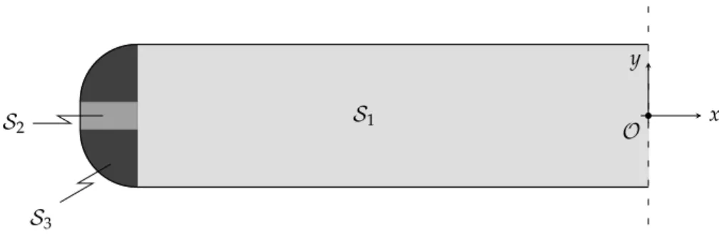
- Geometrical Model and Boundary Conditions
- STAR-CCM+ Numerical Model
- Finite-Volume Method and Unstructured Mesh
- Mesh Arrangement
- Discretization Method
- Pressure-Velocity Coupling
- Solving the System of Equation
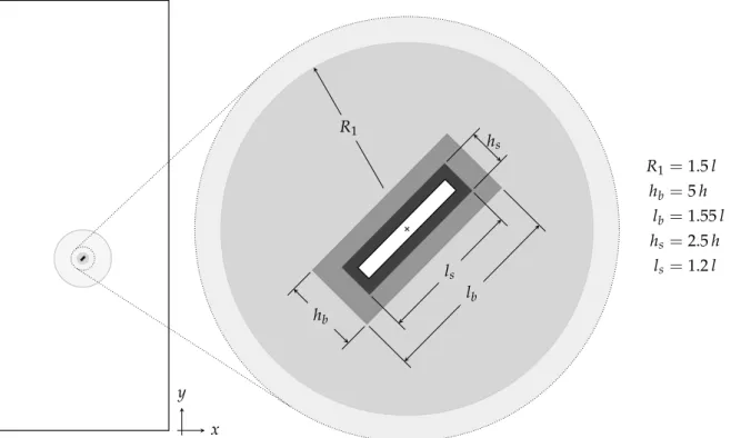
It consists of a floating object mounted on a disk that can rotate relative to the rest of the mesh. A view of the entire domain is shown on the left, while a zoom of the internal drive is shown on the right. In addition, the figure lists the values of the different dimensions, all expressed in plate length.
Then, in the following time step, an upgrade of the relative position between each other and a new temporary association will be made. This condition is applied to both the leading and trailing surfaces of the computational domain and is fundamental to performing two-dimensional simulations. In this work, the first-order scheme was initially used, but due to the poor accuracy results, the second-order scheme has been chosen.
The choice depends on the maximum angular velocity of the plate: to minimize numerical errors, the internal rotating circle cannot shift more than a quarter of the cell to the outside at a time. For a tumbling plate, the angular velocity is higher and, in addition to the smaller size of the internal disk, smaller time steps are required. The nominal value of the convection is calculated by adding to the upstream value a term found by a linear interpolation of the gradients.
The scheme is an improvement of the first order upwind, but some numerical diffusion may still exist especially for high gradients. To achieve this goal, it is necessary to introduce a term that takes into account the non-orthogonality of the vector connecting two adjacent cell centers to the control volume boundary. By solving the pressure correction equation (derived from the continuity equation), the velocities will be upgraded (corrector).
Due to the large size of the matrices involved, the solution cannot be found directly and iterative methods are used.

Validation Study
- Reference Model
- Meshes
- Results
In (a), we can see the prism layers at the slip boundary as well as the enhancement zones around the slab. In order to reduce interpolation errors, 2 prism layers are also used in each region according to the sliding boundary (a). In the following, the results obtained with the finest mesh will be presented in detail.
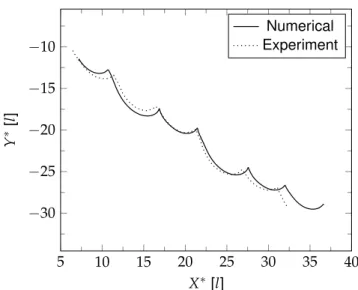
It is important to note that trajectories do not start at the origin of the coordinate system. This is because we are interested in the periodic state and at first moments the plate motion is not well defined. The next step is to compare the trend of dimensionless fluid forces with what is found in the literature.
According to the comparison with the numerical results, the curve shapes are similar especially for Fy. As for the hydrodynamic force along the x axis, we notice that the shape is not exactly the same: our results present a softer valley along the piece and there is no decrease in value in the second period. The results are compared with the experimental ones discovered by Andersenet et al. [21]. (plots on the left).
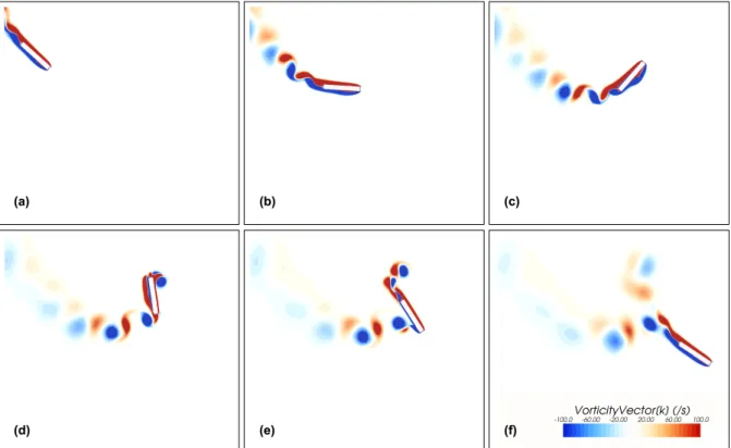
The results are compared with the experimental findings of Andersen et al.[21] (to the left). In Figure 3.5, the fluid torque is compared with the results from the same authors. Note how the wake is always characterized by the shedding of vortices that interact heavily with the plate during rotation at the center of mass peaks.
As the plate accelerates, a new vortex region with the opposite sign (red) is formed, and the old vortex (blue) falls on top of the plate.
Uncertainty Quantification
- Introduction
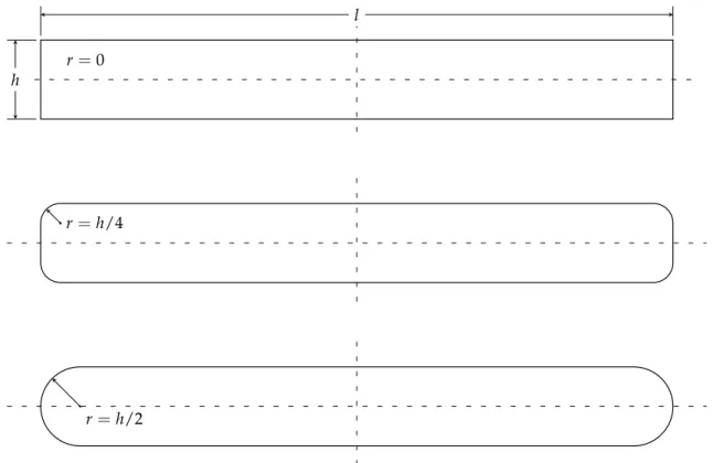
- Geometries
- Mathematical Formulation
- Results
- Tumbling Plate
- Fluttering Plate
Let us consider the uncertainty parameter of the model that it is associated with the random variable ξ. Considering Legendre polynomials, they have an important property which is the basis of the present formulation. Let us introduce a new variable, the solution of the system, f which from the previous considerations is
Listed on the right are the coefficients of the solution calculated at three different times, T∗ = 40, T∗ = 80 and T∗ =120. Now the graph on the left shows that the trend is not linear: a small variation or the rounding radius in the low range has a much larger influence of the same variation for larger ones. The procedure is exactly the same as in the three-point case: initially we look for the convergence of the solution as a function of time and only then is the stochastic solution that results when falling from a certain height is calculated.
On the right side the five coefficients of the solution found at the three different times are shown. The five coefficients of the solutions calculated in those intervals are plotted on a bar chart. We can see how the stochastic mean, fˆ0, is the main term and that the coefficient of the linear polynomial, fˆ1, plays an important role.
The bar diagram shows how the modulus of the five solution coefficients becomes smaller and smaller as the polynomial degree increases. As briefly written in the beginning of this section, one of the goals of this study is to find the PDF that describes the X∗ solution when a prescribed trap is imposed. From Figure 4.11 it is possible to notice how ther4andr5plate does not reach the lower Y∗ coordinate, so an extension of the physical time to 7s (T∗=177.6) and 8s(T∗=202.9) respectively was necessary.
Therefore, we assumed that convergence is achieved and we can conclude that the system does not follow a linear law, but there is a concentration of events according to extreme intervals (bimodal distribution). In summary, we can conclude that since the geometry of the body is slightly different, so will the vorticity field around the plate. To understand the importance of vortex shedding in flapping regimes, three quiescent plates were considered and simulations were performed.
Conclusions
- Summary
- Main Conclusions
- Future Work
The adopted numerical methodology provided realistic results for two-dimensional tumbling plate and the model can correctly predict the trajectory, the forces and the torque acting on the body. The predictions agree well with experimental data; results confirm and detail how the washwater is controlled by a vortex shedding process. In the tumble case, the fillet angle changes the mean trajectory angle and angular rotation modulus highly.
We attribute this fact to the different wake structure caused by the different angular sharpness, which causes different flow separation processes. In flutter, the locus of the second sliding peaks exhibits an unexpected behavior enclosed in the interval [0.50h2 0.77h2]. The wake investigation shows that the vorticity field around the plate is characterized by a wake-body interaction that perturbed the trajectories.
In a tumbling motion, five points are enough to correctly find the solution with the NISP approach, and the results show the bimodal trajectory and the increasing error bar. The system is characterized by high variability and small perturbations in the geometry (input) cause large variations in the trajectory (output) that underlie how the system is highly nonlinear. After the second slide, an apparently chaotic behavior is observed that can be elucidated with stochastic calculations, but requires a limited number of simulations.
Future studies could consider the three-dimensional case involving more complex wake structures. Additionally, it could be interesting to study bark fall where some model parameters such as initial orientation or wind speed can be modeled using the NISP approach.
Dimensional Analysis
Bibliography
Hirsch.Numerical Computation of Internal and External Flows: The Fundamentals of Computational Fluid Dynamics.