Rational expectations and the service of public debt: a recursive approach

By Lygia Bruno Lobo

Dept. of Economics University ofMiami Coral Gables, Florida

Abstract

This paper uses dynamic programming to study the time consistency of optimal macroeconomic policy in economies with recurring public deficits. To this end, a general equilibrium recursive model introduced in Chang (1998) is extended to include govemment bonds and production. The original mode! presents a Sidrauski economy with money and transfers only, implying that the need for govemment fmancing through the inflation tax is minimal. The extended model introduces govemment expenditures and a deficit-financing scheme, analyzing the Sargent-Wallace (1981) problem: recurring deficits may lead the govemment to default on part of its public debt through inflation. The methodology allows for the computation of the set of alI sustainable stabilization plans even when the govemment cannot pre-commit to an optimal inflation path. This is done through value function iterations, which can be done on a computeI. The parameters of the extended model are calibrated with Brazilian data, using as case study three Brazilian stabilization attempts: the Cruzado (1986), Collor (1990) and the Real (1994) plans. The calibration of the parameters of the extended model is straightforward, but its numerical solution proves unfeasible due to a dimensionality problem in the algorithm arising from limitations of available computer technology. However, a numerical solution using the original algorithm and some calibrated parameters is obtained. Results indicate that in the absence of govemment bonds or production only the Real Plan is sustainable in the long run. The numerical solution of the extended algorithm is left for future research.

December,2000 © AlI rights reserved

1. Introduction

Economists have continually studied the optimality of macroeconomic policy. One important facet of this study involves the time consistency of optimal policies associated with the financing of public deficits. Macroeconomic theory predicts that permanent fiscal deficits may induce an economy to default implicitly on its debt through inflation. Rational agents, who have expectations about the probability of default, tak:e a gamble when purchasing govemment bonds and an equilibrium is attained in the economy. The purpose of this paper is two fold: first, to extend a model introduced in Chang (1998) to include government bonds and production to study this problem in a recursive dynamic analytical framework; second, to use the Brazilian experience to test its feasibility. The new model uses as a point of departure (1) the recursive model developed in Chang (1998) based on Calvo (1978); (2) a two-period model introduced in Calvo (1988). The latter studies the interaction between rational agents and government authorities in a public deficit fmancing scheme in which there is a likelihood of default on public debt. It allows for the possibility of two equilibria: a good, Pareto-optimal one with low interest rates and inflation, and a bad Pareto-inefficient equilibriurn, with high interest rates and high inflation, an implicit default. Calvo concludes that in the absence of govemment pre-commitment, characterized through the issuance of indexed-bonds or an upper bound on interest rates, the economy settles in the Pareto-inefficient one, a dynamically inconsistent result. One problem with this model is that it does not allow for the confrontation of his hypothesis with time series data.

To confront Calvo's hypothesis with time-series data, Chang (1998) is extended to include non- indexed government bonds and production and is calibrated with Brazilian data. Chang (1998) is based on Calvo (1978), which assumes a simple Sidrauski economy with money and transfers only. The absence of govemment expenditures in the model eliminates the need for an onerous deficit-financing scheme through the implementation of heavy inflation taxes. The extended model attempts to address the Sargent-Wallace (1981) problem posed in Calvo (1988) from a recursive dynamic perspective. The extended model is calibrated with Brazilian data using as case studies three Brazilian stabilization attempts: the Cruzado (1986), the Collor (1990), and the Real plans (1994). The advantage of the new formulation is that it allows for the computation of the set of alI dynamically consistent government plans, even when the govemment cannot pre-commit to an optimal inflation path. This is obtained through value function iteration, done on a computer. The numerical solution of the original model was straight-forward. Results obtained indicate that in the absence of govemment bonds or production, only the Real Plan is sustainable in the long run. The Brazilian experience supports well the predictions of the model: that macroeconomic policies that deviate an from optimal path may not be sustainable in the long run. The numerical solution of the extended model proves unfeasible due to a dimensionality problem in the algorithm arising from limitations in the available computer technology and is left for future research.

2. The model

Time is discrete and there are infinite periods: t

=

0,1,2, ... ,00. There is a welfare maximizing governrnent

in a closed economy who sets marginal tax rates and seignorage to smooth out the tax burden over time. There is one representative consumer and one consumption good that is consumed or invested. There is production given by

F(k

f ) , the only source of income. There is depreciation, Õ, and no population growth. There are two assets:

money and nominal governrnent bonds. Households take initial capital stock,

k

_{o '} initial money holdings,

Mo,

initial stock of governrnent bonds,

b

_o

= O ,

and marginal tax rate, r f as given.

Preferences:

The representative household's preferences over consumption and money holding are given by

2.J3'[u(c, )+v(m,)] ,:0

Functions u and v satisfy:

(1) u: 91+ ｾ＠ 91 is CJ, strictly concave, and strictly increasing.

(2) v: 91+ ｾ＠ 91 is CJ

, and strictly concave.

(3) Um u' (c) = Lim v' (m) = 00

c-+O m -+0

(4) There is a finite satiation levei ofmoney,

rrI >

O such that v'

(rrI)

= O

Furthermore, consumption, the price levei and the real value of money holding at the end of period t are

respectively given by c" p'. m, where

M,

m,

=--p,

q,

=.l-.,

the inverse of the price levei

Pt

Money supply:

Money grows at a constant rate J.l, .

Real money growth, inflation and the satiation levei of money holdings are respectively given by

P,+I (I )

--m,+1 = + J.l, m, p,

7r

_,

= (p'+J - p, ) p,

Government Bonds:

Bonds are one-period to maturity, zero coupon government bonds, where

QI

=

$1 is the normalized price of a bond

BI is the number ofbonds

b_l

ｾ＠

is the real value of a bond at period t

P

I

R

=

(

1 - QI) is nominal retum on bonds at period t

nI

QI

(J + rgt) = (J + Rnl}PI

PI+I

. th I f b ds (1 ) (J + Rnl)

IS e rea rate o retum on on ,or + r = ＮＮＮＺＮＮＮＮＭ｟ＮＮＮＮＡＡＡＮＮＮ［ｾ＠

gt (1 + 1f

1 )

is the real present value of a bond that matures at period t+ 1

(J+rgt)

b_o =

O

is the initial stock ofbonds

b

=

bf > O is ao upper bound on bond holdings

Taxes

rI is a proportional tax levied at each period t. Consumers take rI as given.

rI

F(k

_l ) is the total tax revenue, a fraction oftotal production.

Deficit financing

The leveI of

g

I at each period t is a government decision exogenous to the model. At each period, the

government chooses how much money to create or to withdraw from circulation aod how many bonds to issue or to retire, aod must satisfy:

Default

ｾ＠

is the share ofbonds not defaulted at period t PI+I

The consumer problem The household will maximize

Ip'

[u(c,} + v(m,}} S.t.

,=0

k

ｾＫＱ＠

(

c, + ,+1 +(J+7r, }m'+1 + (J ) = l-r, }F(k, }+k +m+b,

+rgt '

k,

=

(J - t5 }k,

+

i

The government problem

Govemment will maximize its representative consumers' utility

I

P'

[u( c, ) + v( m,)} S.t. ,=o

g, - r, F (k, )

= [

b'+l - b,

J

+ [(1

+

7r, }m'+1 - m,

J

where (J+rgt)

g, - r, F( k, ) is the govemment primary deficit at period t

The consumer value function: States: k ,m ,b

ControIs: c', k', m', b'

Prices: p ,p'

V(k,m,b}

=

Max {u[O - r }F(k} + m + b + k - [k' + (1 + 7r }m' + b'

II

+ v(m)

k'.m'b'

0+

rg}

+ V(k',m',b')}

FOC's:

k': (-l)u_c[( l-r )F(k)+m +b - [k' +(1 +7r )m' + b'

II

+ PVk(k',m',b') = O (l + rg)

b'

m': -( 1 +7r}uJ( l-r )F(k) + m +b +k - [k' +( 1 + 7r )m' +

II

+ PVm(k',m',b') = O (J + rg)

b'; -(1) uJ(J-r}F(k)+m+b+k-[k'+(J+7r)m'+ b' }]+pV_h (k',m',b') = O

(l + r ) (1 + rg)

g

The government value function:

b'

W(m,b)

=

Max {u[(J - r ))F(k+ m +b + k - [k' +(1 + 7r}m' +

II

+ v(m)

h'.T (J + rg)

+

W(m',b') }s.t.

b'

g-rF(k)=[ -b]+[(J+7r)m'-m}

Competitive Equilibrium

A policy is a sequence of nominal money growth rates, J.i = ( J.io' J.i1 , .. .), a sequence of tax rates,

r=('o,r1 ,··.) andasequenceofbonds

b=(bo,b\

, ... )

s.t. J..l E [li,!:!.] == [fl,!J..) ==

n

｡ｮ､｡ｬｬｴｾｏＮ＠ An

al/ocation is a set of nonnegative sequences of consumptionc=(c_O'c_{1 , •• .),} capital, k=(k_{o,k1, .. .),} real money

Given an initial capital stock, _ko, an initial nominal money holding Mo, an initial stock of bonds, _bo = O, and a govemment policy (f.i, 1; b), a CE is formed by an aIlocation (c, k, m, b), a value function Vand a vector of

prices (7r, r g) if:

(i) The FOC's ofthe consumer problem are satisfied:

(1) k':(-I)uJc)+f3V (k',m',b')=O

k

(2) m':(-l)(l+7r)uJc)+f3V (k',m',b')=O

m

(3) b': (-1) _{uc(c)+f3V (k',m',b')=O}

(J + rg) b

(ii) Markets clear every period:

(4) Money demand equals money supply:

(1 + J.i, )

m

=

m

,+1 (1 + 7r,) ,

(5) Bond demand equals to bond supply:

b'+I=(l+rgr){g, -r,F(k,)+b, -[(I+7r,)m'+I-m,)}

(6) Total expenditures equals total resources:

c,

+

k'+1 = F(k, ) - r, F(k, )

The Continuation Value of Equilibrium

The continuation of a CE is a CE. In other words, if (m, T, f.i, b) E CE, then (m,,!i, ｊＮｩｾ＠ b) E CE. FoIlowing

Chang (1998), the continuation value of equilibrium, wiIl be used as an artificial state variable in the Ramsey problem with bonds. The three envelope conditions wiIl yield a vector of promises made at period t: the promised marginal value of capital, the promised marginal utility of money, and the promised marginal value of bonds, respectively given by

V =[(l-r)F (k)]u (c)=4/

k k c k

V =u (c)+v (m)=4/

c m m

V =u (c)=4/

b c b

Steady State

In steady state C'+1

=

c,

=

C, k'+1

=

k,

=

k, m'+1

=

m,

=

m, and b'+1

=

b,

=

b . These are obtained from the solution of the system of equations and unknowns formed by the definition of CE. The equilibrium conditions for the money and bonds market given for the maxirnization problem above are respectively

(1+J.i, )

m

=

m

,+1 (J+Jr,) ,

The simplified Steady State consumer Euler equations are:

- J

-k : - = (1- , )Fk (k)

fi

The Ramsey Problem with goveroment bonds and perfect commitment:

Under perfect commitment the govemment's problem is to choose a policy J.i and an associated CE such that there is no other CE that results in higher consumer welfare.

The problem is to choose (m, r, f.J, b) in CE to maximize

2..13'

[u(c, )+v(m,)} s.t.

,;0

C, +k'+1 = F(k, )-" F(k, )

The Ramsey problem must be solved recursively. From the FOC's and the continuation value of equilibrium defioed above we have that all the promises made at t are given by:

( J -', )Fk (k[ ) = ｲＯｊｾ＠ ,the promised marginal value of capital u c ( C )

+

V m (m) =

r/J

ｾ＠

,

the promised marginal utility of money

uJ c) = ｲＯｊｾ＠ ,the promised marginal value ofbonds

r/J'

=

(r/J;

ＬｲＯｊｾ＠ ＬｲＯｊｾ＠

),

the vector ofpromises made at period t

Let the set of initial promises consistent with CE be defrned by

n,

where 3( m, ',J1, b) E Q :

Q = tm", J.i,b) E CE Ir/J E 913 : (({( J -'o )F_k (k o )JuJ Co )),(uJ co) +vm(mo )),(u_c (co ))}

*

Maximize

LJ3'

(u(c, )+v(m,)} s.l. ,=0

fjJ = (fjJk ,fjJm' fjJb ) , a vector of initial promises, and T(fjJ)= {(m, ,T, ,p, ,b, )ECE IfjJ=(fjJk,fjJm,fjJb))

Therefore, r(fjJ)= {(m, ,T, ,p, ,b, )ECE _{IfjJ=({(J-To)Fk (ko)}uJco)),(uJcO)+vm(mo)),(uJco)))}

Given a vector of initial promises fjJ = (fjJk ,fjJm ,fjJb) in Q, T( fjJ) is a non-empty, compact subset of CE.

*

*

Since the objective function is continuous, W (fjJ) is well defmed on Q. If W () were known, then the problem

*

would be to obtain the max of W (fjJ) on Q . Thus, a dynamic programming formulation can be obtained.

*

W (fjJ) satisfies the functional equation W(fjJ) = Max ({u(c) + v(m)}+f3W(fjJ')) s.t.

1) (m, T,p,b,fjJ') E ExQ

2) fjJ=(fjJk,fjJm,fjJb) where fjJk =(J-T)Fk (k)uJc)

fjJm =uJc)+v",(m)

fjJb =uJc)

b'

3) g-TF(k)={ -b}+{(J+7r)m'+m}

(J

+

rg )

4) (J-T)Fk(k)uJc)=f3fjJ;

uJc)+v,Jm)= ｦＳｦｪｊｾ＠

uJc)=f3fjJ;

*

If a bounded function W : Q ｾ＠ 9t 3 O;atisfies the above functional equation, then W = W . If the set of

all possible artificial states Q can be computed, the Ramsey problem can be solved recursively. The set Q can

be computed by using the fact that it is the fixed point of a particular operator.1 _{Let W be a subset of 9t} 3 . A

new subset B(W) will be defined as:

B(W)={fjJE'J{3 :3(m,r,f.l,b,fjJ')EExW

I

fjJk = _{(1-r)Fk (k)uJc)}

fjJm =uJc)+vm(m)

fjJb=UJC)

b'

g - rF (k ) = [ b} + [ (1 + 7r )m' + m) and

(1 +rg)

(1-r)Fk (kJuJc)=fJfjJ;

uc(c)+vm(m) = ｦｊｦｪｊｾ＠

uJc)=fJfjJ; hold}

Then, W ç ｂＨｗＩｾ＠ B(W) ç and =B( )

Thus, .Q can be computed by iterating on B. Once

n

is known, the functional equation can be solved to

*

obtain W . The introduction of the vector of artificial state variables

fjJ

=

(fjJk ,fjJm,fjJb)

takes care of the requirement that the new Ramsey Problem must be consistent with a perfect-foresight CE.

The Ramsey Problem with no Pre-commitment

Next we assume that the governrnent cannot pre-commit to an infinite policy sequence. The CE is defined as a set of Sustainable Plans as described below.2 The goal is to compute the set of alI SPs recursively. The incentive constraint is handled through the introduction of the continuation value of the equilibrium, which is the vector ofpromises fjJ = (fjJk ,fjJm.fjJb) and is used as artificial state variables. After any history, the continuation of a

SP must be consistent with a CE for the infmite future. To ensure CE for the infmite future, the set of SPs must include two vectors of artificial state variables. The first is the one corresponds to the three FOC's; the second is the vector promises made at period t. The SPs and sustainable outcomes will be defined next.

Sustainable Plans

Sustainable Plans will now be defined as in Chang (1998). Let a money growth history and a govemment strategy be defined as:

History: f.l'

= (

f.lo' f.ll , ... , f.l, ) , restricted to f.l E

("ji,!:!)

=

(if, ｾ＠

=

Il

Strategy: a' =(ao,al, ... ,a,) suchthat ao Elland a, :ll,-I ｾｉｬ＠

The strategy space available to the govemment will be restricted to those consistent with CE. 3

2 Procedure is the same as in Chang (1998)

Let

CEn

be the set ofinfrnite horizon sequences ofrnoney growth consistent with CE. Thus,let

CE n = (3( f.i, m, i,b )I(m, i,b) E CE}

A strategy

a'

is admissible if after any history f.iH, the continuation of

1./

E

CEn.

Ao allocation rule a is a sequence a=(ao,al, ... ,a, )s.t. for each t, a, :IJ' ｾＨｏＬｭｊ＠ )xix(O,bJ ) ,

where a, ( f.i' ) = {m, ( f.i' ), i , ( f.i' ), b, ( J./)} denotes the real value of money, taxes and bonds respectively. Next, the governrnent will be restricted to choose an admissible policy. It will announce for the future a policy that is consistent with the existence of CE. A governrnent strategy a and an allocation rule a constitute a Sustaioable Pia0 if:

(i) ais admissible

(ii) a is competitive given the strategy a

After any history f.i ,-I , the continuation of a is optimal for the governrnent, that is, the sequence f.i,

induced by the strategy aafter a money growth history f.i,-I maximizes

Ip'

fu(e, )+v(m,)] over _{CEn ,} given a. ,=0

The continuation of a SP is a SP. Thus, any SP induces a CE sequence (m, r; J.i, b) and any CE sequence is a sustaioable outcome ifinduced by some SP.4 Next, the SP is characterized recursively.

Consider frrst a "best" deviation. Let

e

= {(m, r; J.i, b) E CE

I

:3

a SP whose outcome is (m, r; J.i, b) } be the set of all sustainable outcornes. Defme S as

S = {(

w,

<p)

I

:3

a SO (m, "t, /l, b) E

e

with W s.t.

r/J

= (

_{r/Jk ,r/Jm.r/Jb}

) ,

the vector of promises made at t}

The set S is the set of all pairs of continuation values and promises that may emerge in the frrst period of a SP. S will be characterized in a recursive way. Aoy SO implies an initial value Wand an initial promise <!l. The pair (W,

<p)

must belong to S.

In the frrst period, a SP must describe an initial optimal action J1i and for each possible deviation fiom f.ii '

i.e., each f.i E CE o , the SP must specify the real quantity of rnoney m( f.i) , taxes a( f.i) and bonds b( f.i). The SP will specify a continuation value, W ( f.i) and a continuation "promise" <P'+I ( J1), which must belong to S. Let Z

I . I

denote a subset of W x Q .Define a new set D as

D (Z) ｾ＠ WxQ

4 This follows from the Abreu, Pearce & Stachetti operator described in Chang (1998). The existence of SPs has already been

D (Z)={ (W, 41 )

I

3 a J.I E CEO, and for each p E Ce

,:3

a vector (m( p), a( p) ,b( p), ｾＫｬ＠ p), 41,j p)) in (O,nl) x T x (0,11) x Z s.t.:

1) W = u (e(p) + v (m (J.I))j + ｾ＠ W' (p) 2) 41 = (41k ,41m.41b)' where

3)

41k = _{[(1-r(p))Fk (k)]uc(e(p))}

41m = uJe( p))+vm(m( p))

41b =uJe(p))} andforall pE CEo,

W ｾ＠ u [e(p)]

+

v [m (p)]

+

ｾ＠ W'(p)

4) g-T(p)F(k)=[ b'(p) b(p)} +[(1 +7r(p))m' +m(p)}

(1 +rg)

5) (1- T( P _{)Fk (k)uJ} e( p)) =

/3ifJ;

Uc (e( p))

+

V m (m( p)) = ＯＳｩｦｊｾ＠ uJ c( p)) = P41;

Constraints 4 & 5 are necessary to ensure that the continuation of a SP after any deviation is consistent with a CE. IfZ ç D (Z), then D (Z) ç S and S = D (S), S is the largest fixed point ofD.

The algorithm to compute S is given by S o = W x.Q , S n

=

D( S n-} ), n

= }

,2,... The sequence converges to S.

Therefore, it is possible to compute S and a SP corresponding to any (W, 41) in S

Next, consider a deviation that minimizes welfare losses to society. 5Let p be a deviation from equilibrium. Let Z be a compact set S.t. S ç Z ç W x.Q . Defme P as

P (p; Z) = Min u [e]

+

v (m)

+

ｾ＠ W' S.t

b'

b} +[(1+7r)m'+m)

1) g-TF(k)=[

(1 +rg)

2) (m, r, b, W,+1. 41,+1) E (O, nl) x T x (O,h') x Z

3) (1-T)Fk (k)uJc)=P41;

4) U_c (c )+vm(m) = ｐＴＱｾ＠

5) uc(c)=P41;

If Z were equal to S, then P(j.J; Z ) would be the worst possible continuation after the deviation h in CEo 1[ •

This is extended to allow for punishments supported by (W, 41) in sets Z > S. Let

BR (Z) = Max P (p; Z ) subject to !l E

cEg

If Z = S, then BR (Z ) would be the govemment's best deviation. Finally, define E (Z) as

ｅＨｚＩ］ｻＨｗＬｾＩｅ＠

wxnl

:3

(m, T,f1,b, W',B')EE

x

Z s.t.allthefollowingconditionshold:

1)

2)

3) 4) 5) 6)

b'

g -rF(k) = [

bJ

+ [(l +7r)m' +m)

(l +rg)

(l-r )Fk (kJuJc) = ｦＳｾｾ＠

uJc)+vm(m) = ｦＳｾＺ＠

uJc)= ｦＳｾ［＠

w

= u (c) + v (m) + ｾ＠

w'

ｾｫ＠ =(l-r)Fk (k)uJc)

ｾｭ＠ =uJc)+vm(m)

ｾ｢＠ =uJc)

7) and

W?

BR (Z) }

If Z = S, E (Z) would include all pairs (W, ｾＩ＠ that could be enforced by a threat of reverting to the least favorable continuation for the govemment. To obtain the algorithm, we use the fact that

S ç Wxil and Zo = Wxil. For all n = 1,2, Zn = E(Zn_1)

3. Calibration

The calibration procedures conducted herein follow standard guidelines present in the literature,6 _and

involve mapping the model into observed features of the Brazilian data. Going from the theoretical framework to the quantitative analysis involves three steps: first, choosing a parametric c1ass; second, constructing data measurements that are consistent with the parametric c1ass chosen, establishing a correspondence between the parametric c1ass chosen and the observed data. This requires re-organizing the data in such way that is consistent with the model; finally, assigning values to the above-mentioned parameters of the model, which involves setting parameter values so that the behavior ofthe model matches the features ofthe measured data. For this model economy, this implies estimating values to the parameters oftechnology, productivity A, capital share, B, depreciation 8, preferences, a, p,

/3,

and tax policy, r. 7

3.1 Functional Forros

The OOt step in the calibration procedure is to choose the functional forros used. The analytical framework under1ying the mode1 developed herein involves utility maximization with money in the utility function in a monetary economy with production and two assets: money and bonds. Functional forros were chosen to ensure that assumptions (1)-(4) ofthe theoretical model, as described in Chapter 3, are meto

Utility:

Utility is represented by

U( c, ,m, ) = u( c, )+v(m, )

where

u( c, ) = log( c)

mf is the satiation leveI of money

Production:

The modeI assumes a Cobb-Douglas production function with constant returns to scale and depreciation (ó).

K is the total capital stock

L is the economically active population.

A is a measure of average overall technoIogical change or average productivity

6 Kydland & Prescott (1982), Cooley & Hansen (1992)

() is share of capital in measured GDP 8 is the depreciation rate

In per worker terros, the production function becomes

K

F(k)=Ae , where k=-L

3.2 Calibration of the Parameters The next step is to calibrate the parameters:

Preferences: p, fJ, a Technology: B, A, 8

Policy: f.1, T

Preferences: Utility is given by

LU(C, )+v(ml ) where

1:0

m2 v(m

)=am+-1

2

Thus, the discounted lifetime utility becomes

ip,

[zn(C

1 )+[m

ｭＫｾＱＱ＠

1:0 f 2

The simplified steady state consumer Euler equations obtained above are:

- 1

-k :

p

= {l - T )F_k (k )

-

(-)

p

(-m : U_c c = V_m m)

(l+1r-P)

- 1

b:-={l+p)

p

The subjective rate of time preference , p -in steady state, return to govemment bonds is equal to return to capital.

The discount factor,

f3

-

was estimated as per the definition 1

p =

The satiation levei of money, ID,: - was calibrated using the simplified steady state euler equation :

uJc) = (J+:-fJ) vm(m)

(_ 1 uc c)=-:=

c

1 fJ { -}

ｾ］＠ l+1(-fJ

mf-m

ç

= fJ (J+1(-fJ)

1 _

m_f =-+m

cç

c=j(k)-&-(g+X) or

c=j(k)-i-(g+X)

where i is the net investment per quarter, or gross investment less depreciation.

Technology: the share of capital (} and productivity parameter A - were initially calibrated by regressing real GDP on net fixed capital stock and economically active population. Originally, quarterly data was used. Since these parameters do not enter the numerical solution using the original algorithm, this was not re-calculated with yearly data.

l+p=(J-r)F_k (k)

F(k)=Ak'l Lny = LnA + BLnk

Depreciation (Ô) - A quarterly series based on average yearly leveIs was constructed using as point of departure the gross capital stock and net capital stock series constructed by IPEA.

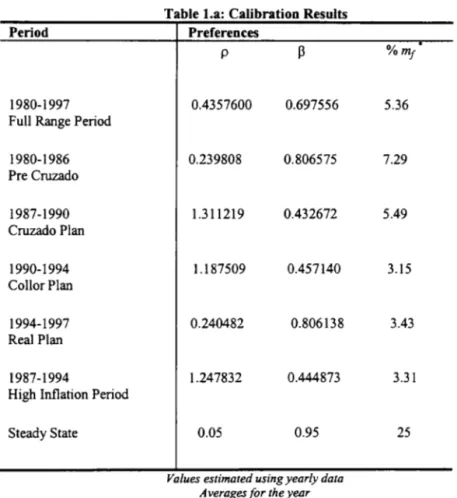
3.3 Calibration Results

near a steady state during this period. Consequently, the results obtained in the fust calibration attempt (1980-1997) presented distortions reflecting these facts. For this reason, the fundamental parameters

P

and mf were calibrated

again using data from the 50s and 60s, when the economy resembled closer steady state equilibrium. Calibration results are reported on Table 1. Sample averages are reported on Table 2.

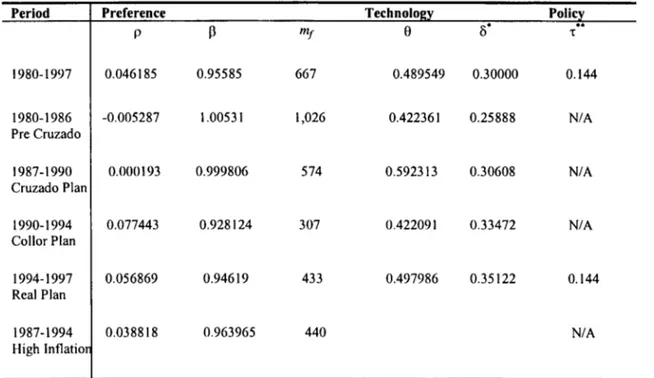
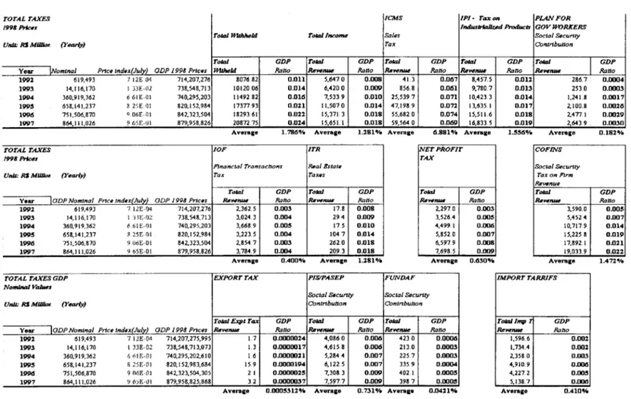
The estimation of the preference parameters was straightforward. The parameters p and f3 followed directly from the assumption that in steady state all interest rates in the economy are equal. Real interest rates were estimates from the Fisher equation, by obtaining the difference between the nominal interest rates on govemment bonds and inflation. The Cobb-Douglas production function parameters were obtained by running a standard restricted form of the growth accounting regression, by regressing per worker output growth, log (f/L), on capital per worker growth, log (KlL). The full-range sample was used as reference model. The Durbin-Watson for the initial specification ofthe reference model indicated the presence of serial correlation, indicating that different factors other than capital and labor affected output, These could include the institutional framework underlying the different stabilization attempts. The most difficult parameter to calibrate was the average tax rate, r.. This was due to the fact that several taxes were created and eliminated during the period studied, making their consolidation extremely difficult. Historical data on taxes that are no longer in effect (for example, the export tax) is no longer available from the usual sources prior to 1992. Historical series are available only for total federal fiscal income prior to 1992. Historical data for state and municipal taxes are not available, with the exception of sales taxo Obtaining and consolidating this information would require an amount effort and time beyond what is feasible for the conclusion of this paper, and will be left for future research. Since taxes do not affect the steady state equilibrium of the model, a narrower period range for the study was allowed. This made possible estimating the averages with the exiting data sets, since the narrower data range does not affect the steady state equilibrium or the numerical solution of the model and results. The calibrated tax parameter was 14.5%. Due to these problerns, the tax rate calibrated herein is underestimated, but can be used as a point of departure for this research. The breakdown of the tax structure is reported on Table 3. Figures 1 and 2 summarize data on inflation, interest rates, Ml and govemment bonds.

Figure 1

Quarterly InOation and Nominal Interest Rates, 1980-1998

400

4r---,

300 200 100 o -100 1.4 1.2 1.0 0.8 0.6 0.4 0.2

--- --- --- Inflation _ _ _ _ o Interest Rate

Figure 2

Real Ml and G-Bonds per worker as GDP natio, 1998 Real.

ＬｾＬ＠

I \

1 \

, J \

I

1

\ I

\ _I

....

'

I

"

li " "

,

,

,

,

, , ,

I

,

_,

,

1 1

ＬｾＭ

,

...

'

1'1 I 1

,

1\ } \ I,

,

-'

''''

,

I I ,

I \ '

I I 1

:

ｾ＠ ('

, \ I

,

"

-, \ 1

, \ I

"

\ .... '

\

,

\.., ... ",'

0.0 ;'rT'T'T"T"T"T"I"TT"""rT'TTTT"T"I"TTTT'rT'TTTT"T"I"TTTT'rT'TTTT"T"I"TTTT'rT'TTTT'T'1"TTTT'M"T'TT',.,..,r-ri

Table 1.a: Calibration Results

Period Preferences

p _ｾ＠ %mf

1980-1997 0.4357600 0.697556 5.36

Fu\l Range Period

1980-1986 0.239808 0.806575 7.29

Pre Cruzado

1987-1990 1.311219 0.432672 5.49

Cruzado PJan

1990-1994 1.187509 0.457140 3.15

Co\lorPlan

1994-1997 0.240482 0.806138 3.43

Real Plan

1987-1994 1.247832 0.444873 3.31

High Inflation Period

Steady State 0.05 0.95 25

Values estimated using yearly data Averages for the year

Table I.b: Callbration ResuIts (Quarterly Data)

Perlod Preference Technologl: Policl:

p

{)

o"

""

p mf t

1980-1997 0.046185 0.95585 667 0.489549 0.30000 0.144

1980-1986 -0.005287 1.00531 1,026 0.422361 0.25888 N/A

Pre Cruzado

1987-1990 0.000193 0.999806 574 0.592313 0.30608 N/A

Cruzado P1an

1990-1994 0.077443 0.928124 307 0.422091 0.33472 N/A

Collor Plan

1994-1997 0.056869 0.94619 433 0.497986 0.35122 0.144

Real Plan

1987-1994 0.038818 0.963965 440 N/A

High Inflatio

I

Period

n%

r%

_.

_c

_y

_.

"f ••

_g

_.

_

_m

..

b··

1980-1997 218 43 9,582 12,433 18,057 714 667 1,520

1980-1986 167 24 10,834 14,068 20,736 718 1026 1,304

Pre Cruzado

1987-1989 1052 131 10,445 13,801 19,167 783 574 1,927

Cruzado Plan

r, 1990-1994 1080 119 9,729 12,773 13,279 711 307 1,386

..

-

_{Collor Plan}

C;

n _

t::1'T'

Ze"

1995-1997 7 24 9,451 12,592 16,518 826 433 1,662

ol>

..". _{Real Plan}

ｾｧ＠

ｃｉｾ＠

cn25

1987-1994

I

1066 125 10,087 13,287 16,223 747 440 1,657

!!l::c _{c: IT'} High Inflation

r - Z

- : x l

0 _

< 0

_,.C:

• Values in real terrns per worker, yearly data, 1998 Real

.. Values in real (errns per worker, stock, 1998 Real

::em

cncn

Table 3. Tax Structure

TOTAL TAXES ICMS IPI- Ta:xon PLANFOR

/99B Prlc.. ｉｮｭＮｳｾ､＠ Products GOVWORXERS

Tokzl JtIthIoeId TolallncolfU1 Sa/t1s SocIal s"CUl1ty

UnU: RS M/IlIo. (YmuV) Tax Conlnbutton

Tokzl GDP Tokzl GDP Tokzl GDP Total GDP Total

I

_GDP Ve ... INomlnal PncBlnd.x(July) GDP J 998 pnc .. H1IheId Ratto &WnIII1 Ratto &""1IIM1 Ratto &1'<1_ Ratto &w_ Ratto

1992 619.493 ., 12E 04 714.207.276 80711 82 0.011 5.647 O 0.008 41.3 0.067 8.457.5 0.012 2811.7 0.()()()4

1993 14.1111.170 1 DE·lU 738.548.713 10120011 0.014 11.420 O 0.009 856.8 0.061 9.780.7 0.013 253 O 0.0003

1994 360,9 I 9.362 ti 61E·OI 740.295.203 11492 82 0.016 7.533 9 0.010 25.5397 0.071 10.423.3 0.014 1.241.8 0.0017

1995 658.141.237 8 ＲｾＮｅ＠ 'lI 820.152.984 17377 93 0.021 11.507 O 0.014 47.1989 0.072 13.635.1 0.017 2.100.8 0.0026

1996 751.506.870 006[.·;]1 842.323.504 1829361 0.022 15.371 3 0.018 55.682 O 0.074 15,511.6 0.018 2,477. I 0.0029

1997 864,1 I 1.026 9 ＶｾＬｅＭｬｊｴ＠ 879.958.826 ＲｾＮ＠ 0.024 15.651.1 _--º'º!lI ｾｾＵ￉ＴＮｯＮＭ _ 0.01SlJ _16.833.5 . - 0.019 2,643 9 0.0030

Averaae 1. 786% Averale 1.2810/. Avel'U.le 6.881°/. Averaae 1.556% Avence 0.182'Y.

TOTAL TAXES IOF ITR NETPROFIT COFINS

/99B Prl<;<1S TAX

Mnanc1al TransacHons RIIall!slalll Soctal SflCUrl.ty

UnU: RS MU1Io. (Ytlarly) Tax ｲｑｘｾｓ＠ Taxon P'trm

RI'VfIl'Jue

Tokzl GDP TolaI GDP

v .... anp Nomtnal Pnctllndtlx(JuJy) aDP /998 Prlc.s &1'<111J14 Ralto

&""-

Ratto

Total GDP &""IUIII Ralto

Total GDP

i &""1IUII Rano I

1992 619.493 7 12E·04 714,207.276 2,3112.5 0.003 17.8 0.008 2,297.0 0.003 3,590.0 0.0051

1993 14.116.170 1 " Ｇｅﾷｦｊ［ｾ＠ 738.548.713 3.024.3 0.004 294 0.009 3.526.4 0.005 5.452 ｾ＠ 0.007

1994 360.919.362 661 E·OI 740,295.203 3,6689 0.005 175 0.010 4,499. I 0.006 10.717.9 0.014

1995 658.141.237 ｾ＠ 25E 01 820,152.984 3,2235 0.004 1047 0.014 5,852.0 0.007 15,225 8 0.019

1996 751.506.870 9 UóE·O 1 842,323.504 2.8547 0.003 2112.0 0.018 6,597.9 0.008 17.892.1 0.021

1997 864.1 I 1.026 9 65E·0 1 879.958.826 3.784.9 0.004 209.3 0.018 7.698.5 0.009 19,033.9 0.022

AveralB 0.400'Y. A verale 1.281 % Averale 0.6300/0 Averale 1.472 0/0

TOTAL TAXES GDP EXPORTTAX PIs/PASEP FUNDAF IMPORT TARRlFS

NomJnol Valu<rs

SocIal Secunty SocIal Secunty UnU: RS MUJJm. (YBarly) eonlnbutton Contributton

Tokzl Expt Ta:x GDP Tokzl GDP Tokzl GDP Tokzll"'l' 1 GDP

Voar IODP NomInal pncelnd.x(July) ODP 1998 pnce. &ve1llM1 Ratto &vtlfUIII Ratto &""IUII! Rano &vtl1IIM1 Rabo

1992 619,493 7 I2E·04 714,207,275,995 1.7 0.0000024 4,0811 O 0.006 423 O 0.0006 1.596.6 0.002

1993 14,1111.170 I 33E·02 738,548,713,073 1.3 0.0000017 4,11158 0.006 213.0 0.0003 1.734.4 0.002

1994 360.919.3112 (,líIE·(1J 740.295,202.11 I O 1 11 0.0000021 5.2844 0.007 225.7 0.0003 2.358 O 0.003

1995 658,141.237 j:) 25E·flJ 820, I 52,983,684 159 0.0000194 6,1225 0.007 3359 0.0004 4,910.9 0.0116

l_

751,506.870 9 ｮｾｲＺﾷｩＱＱ＠ 842,323,504,305 2 I 0.0000025 7,308 3 0.009 402. I 0.0005 4.227.2 0.005

1997 8114.1 I 1.026 Y ￓＩｆｾﾷｌＱＱ＠ 879.958.825.868 3.2 0.0000037 7.597.7 0.009 3987 .. 0.0005 5.138.7 0.006

4 Numerical Solution

This section computes the set of sustainable plans S numerically. The objective is two fold: frrst, to compute S using Chang's original algorithm, but with more realistic parameters. Ris original parameterization ofthe model was chosen simply to ensure that the rnathematical assumptions [A1]-[A7t were met, without commitment to a real economy. The original parameterization is:

u( c) = 10,000 log( c)

f(x) = 64 - (O.2x/

x = m(h-1)

m

v(m)=40m--2

p=0.9

II = [Il,!lJ = [0.25,J.25}

The new parameters were obtained from the calibration of the model using Brazilian data. A more ambitious goal was to increase the dimension of the algorithm to include govemment bonds and production, as in the extended theoretical model. This was proven to be extremely difficult due to limitations of the available computer resources, causing the computation time to increase exponentially with the increase of the size of the grid. Rowever, even though the program was not ruo with the inclusion ofbonds or production as in the expanded model, it is explained below how their introduction to the algorithm would be straightforward. The original algorithm was used using some of the calibrated parameters. The exercise allowed for the discussion of dynamic inconsistency of macroeconomic policies in light of the theory proposed by this model, using as case study the Brazilian economic scenario of the last twenty years. The Brazilian experience was tested in order to verify if according to this model the recent stabilization plans would be sustainable in the long ruo. Results indicated that in the absence of govemment bonds or production, only the Real Plan is sustainable in the long ruo. In spite of the computational difficulties found, the exercise was fruitful because it lay the foundation for the nurnerical solution of the extended mode! with the proposed increase in the dimension of the algorithm, which will be pursued in future research

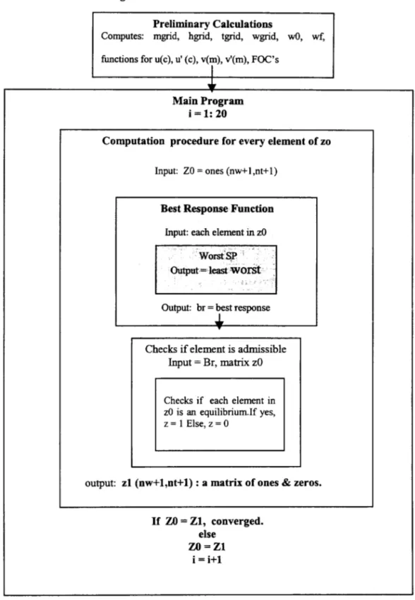
4.1 The algorithm

The structure of the original algorithm is summarized in Figure 4.1. The general idea is that solution of the model is obtained using a grid approach in which the space for the simultaneous solution of the value function and constraints equations is broken into intervals and equilibrium points are searched in each interval. The algorithm is divided into distinct parts. The fust is a subroutine that perfonns some preliminary calculations, which are used later in the program. It begins by computing the grids for money balances, mgrid, and nominal money growth, hgrid.

8 [AI] u:

9t+

ｾ＠

9t

is

C

2 ,strictly concave, and strictly increasing.

[A2] v: 9t + ｾ＠

9t

is

C

2 , and strictly concave.

[A3] Lim u' (c) = Lim v' (m) = a)

c-+O m-+O

Next, it computes the set of possible values of the inflation tax, X, and consumption as a function of the deadweight loss due to the inflation taxo It then computes: u(c), v(m), u'(c) and v'(m); the vector ofpromised marginal utility of money, tgrid, obtained from the estimation of an upper bound for theta, the highest possible promised marginal utility of money from the FOC, (with no inflation tax and highest money holdings, mf); the discounted lifetime utility, wgrid, the non-monetary equilibrium, wO, and the equilibrium under the Friedman mIe,

wf

These are saved for later.

The next block of the algorithm contains a series of subroutines that will compute the set of sustainable plans under no govemment pre-commitment, the set S. It begins introducing a rnatrix Z whose dimension is the length of tgrid x length of wgrid, and whose elements correspond to a pair (8, w), elements in tgrid and wgrid. The program initializes Z as a rnatrix of "ones" in a parent program that will repeat each set of subroutines several times until Z converges to the set S, which is a subset of Z. Within this program there are two distinct blocks. The fust computes the best govemment response function. The key idea is that when considering following an equilibrium recommendation, the govemment considers only the payoffs associated with the "best" deviation: one that minimizes the welfare losses to society. This is obtained through a series of tests. For each element in wgrid and every possible deviation h, the subroutine tests for the "highest" worst possible deviations, as given by equations (18)-(21) in Chang (1998). Given each deviation h, promised marginal utility of money theta, and a desired condition for the "worst" SP, this is computed numerically by testing if the difference between each element in

wgrid and in the rnatrices generated by the set of CE equations computed for the worst possible SP lies within the 10% error tolerance, as in the perfect commitment case. The three matrices generated by this set of equations are: the utility function matrix given by u(c)

+

v(m), the FOC and theta, the artificial constraint rnatrix. For each deviation h, the corresponding column of each one of these matrices is chosen. Every element in each column is tested for the desired condition: that the rnaXÍmum value allowed for w (initialized by wmax) is the minimum element of the utility matrix. AdditionallY' the constrained imposed by the artificial state variable theta is tested against tgrid: the difference between each element in the column of the artificial constraint theta matrix and ｾＪｩｴｨﾭ

element in tgrid is checked to verify if it lies within the 10% error margin. If yes, a "one" is attributed to an index column vector, and a "zero" if otherwise, indicating as before a CE. N ext, the column of minimums is compare with this index vector, and only the elements corresponding to the "ones", i.e. the CE thetas, are chosen. The minimum of these is then chosen as the new maximum W. This value is then compared to a "best" value for w, which is initialized as wmin, the lower bound on wgrid. If this best value is srnaller than the new rnaximum w computed above, then the new best becomes this value. This procedure is repeated for the next deviation h. Thus, the output of this block is a scalar, which is the best value for w and is used in the next block.

error tolerance. If yes, a "one" is given, and a "zero" otherwise. The result is a matrix of ones and zeros, where as before, ones correspond to equilibrium points. These procedures are repeated until Z converges to the set S.

The main problem with this algorithm is the number of times these subroutines must be repeated, generating endless loops, which become difficult to compute with the available computer technology. The original model, based on Calvo (1978), presents a Sidrauski economy with money and govemment transfers only, implying only one FOC and implying 2 artificial constraints only. Increasing the dimensionality in the model with the introduction of bonds and/or production is theoretically straightforward but would make the numerical calculations even more difficult, since it would involve more implicit loops. The introduction of govemment bonds in the budget constraint would involve the introduction of another FOC equation, and in turn 2 more artificial state variables. Likewise, the introduction of production would involve another FOC and 2 more artificial state variables. For each of these artificial state variables there would be a corresponding matrix whose every element would need to be tested as described above. This would also involve an increase the dimension ofthe original E-grid matrix (m x h) to (m x h x b ... ) The numerical computations involved in increasing the dimensionality of the model to this extent have proven unfeasible with the available technology. Due to these difficulties, the actual computation of the algorithm was conducted only with the new estirnated parameters, leaving the expansion in the dimensionality of the algorithm for future research.

Figure 4.1 Structure of the Algorithm

Preliminary Calculations

Computes: mgrid, hgrid, tgrid, wgrid, wO, wf,

functions for u(c), u' (c), vem), v'(m), FOC's

I

Main Program

i = 1: 20

Computation procedure for every element of zo

Input: ZO = ones (nw+ I ,nt+ I)

Best Response Function

lnput: each element in zO

Output: br = 1st Tesponse

Checks if element is admissible

Input = Br, matrix zO

Checks if each e1ement in zO is an equilibrium.lf yes, z = I Else, z = O

output: zl (nw+1,nt+1) : a matrix of ones & zeros.

If ZO = Zl, converged. else

ZO=Zl

4.2 N umerical Results

This section summarizes the numerical results from the computed algorithm above. The numerical computations use the parameters estimated above. These parameters are normalized to rnatch Chang's rnaximum feasible output in the original parameterization of the model. He chooses the satiation money to be 62% of the rnaximum feasible output. The mf obtained from the FOC using Brazilian data from the last 20 was about 2% to 5%

ofGDP, which seemed too low. This stemmed from the fact that average money holdings in Brazil were low during and after the hyperinflation years. The next step was to calibrate the parameters using Brazilian data for years prior to the hyperinflation history. The MlIGDP ratio found for the 50s and early 60s was around 25% of GDP, which would yield an estimated mf in the 25% to 35% range using the FOCs of the extended model. Next, US data (for sure, no hyperinflation history there), was checked, and mf was found to be approximately in the same range, approximately 25% - 30% of GDP. Nowhere the MlIGDP ratio in the 62% range used by Chang in the original parameterization of the model was found. Next, historical data for real interest rates in the same periods were checked for years with no hyperinflation history. The conelusion was that the real interest rates for these years would yield

f3

for the US around 0.97, and for Brazil around 0.95, much higher than the values obtained using the data from the last 20 years. The explanation to these findings is that the economic instability of the last 20 years were giving rise to distortions in the calibration of fundamental parameters such as mf and

f3.

The appropriate calibration was done using data from years with no hyperinflation history, whose economic performance resembled eloser a "steady state" economy.

Once all of this was done, a series of exercises was conducted with the algorithm. The program was run again several times with 1/2 of the original grid: mgrid with 60 intervals, hgrid with 30, tgrid with 30, and wgrid

with 29 intervals. The resulting Z rnatrices, the computed sets sustainable plans, S, were 30 x 31 matrices of ones and zeros, again, ones meaning equilibrium points corresponding to a pair (8, w). Two groups of separate tests, each with a different lower bound on the inverse of nominal money growth, h, were conducted. For the first, hmin was set at the original hmin, 0.25, and for the second for the second, hmin was set at 0.03. This was done to avoid ruling out the inverse of rnoney growths observed during the hyperinflation years in Brazil, when nominal money growth rates some periods surpassed 2000% per year, yielding lower bounds for hmin around 0.03. Computations for each of

these two scenarios were placed on two separate panels. For each hmin, the tests were repeated twelve times: for mf

set at the original 40 (62%Y) leveI, and at 26(40%Y), 22 (35%Y) and 16 (25%Y); for each different mfthe tests were repeated for

f3

set at the original 0.9, then at 0.95 and 0.97. For each scenario, the upper bound on the prornised marginal utility of money, thetamax, the minimum possible equilibrium, wmin, the nonmonetary equilibrium, wO, the equilibrium with the Friedman Rule, wf and the highest possible equilibrium, wmax for all tests were computed. Results from these computations are summarized in Table 6.3.1. Each test yielded a Z matrix corresponding to the computed set S. AlI sets were graphed and placed on the corresponding h panel.

yielded lower prooúses of marginal utility of money and lower hmins, i.e., bigher money growth, yielded potentially higher prooúsed marginal utility ofmoney. Higher fls yielded bigher wmin, wO, wfand wmax.

Given these facts, it was easy to compare if plans sustainable with hmin set at 0.25 remained sustainable with lower hmins, higher fls and lower mjS, as well as Chang's conclusions, that the computed sustainable plans lied within the range of wO and wf as in bis original findings. These results did not seem to necessarily hold for all cases. This is observed in Panel 3, for wbich the program was allowed to ruo with the grid the same size as with the original parameters, but now using the parameters which seemed to encompass the Brazilian experience: mf = 16, ｾ＠

=

0.95, hnún

=

0.03. Clearly, the computed sustainable plans were spread over a range much broader than this interval, with approximately 75% ofthe ws lying below the non-monetary equilibrium.

To check for the robustness of Chang's original results, the program was ruo with the original parameterization, but with a 100% increase in the size of each grid: mgrid with 240 points, hgrid with 100, tgrid with 100 and wgrid with 99 intervals. The frrst loop ofthe program took 13 days to ruo in a Unix server with IGIG ofRAM. The program was allowed to ruo for 4 weeks, however, the system crashed before it ended.

The algorithm was used to test for some observed facts of the Brazilian economy in the last 20 years, to check if according to this model, the different stabilization attempts would represent sustainable plans. To do this, the prooúsed marginal utility of money and ws under different stabilization plans were computed. The ws were computed assurning that money balances changed in the years encompassed by each stabilization plan, and remained constant at the last value of the last period for the infmite future. Thus, the discounted lifetime utility, w, and the prooúsed marginal utility ofmoney were computed as follows:

Cruzado Plan:

BCruzado

=

u'(f(X87 )

*

m87

Collor Plan:

Real Plan:

pJ

W = u(

I(

_{X 95 ))} + v(m_{95 )} +

P[

u(

I(

_{X 96 )} + v(m_{96 )]} +---[u(

I(

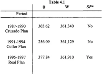
X 97 ) + v(m97 )]

The resulting pairs ((), w) for each case was then compared to the set of sustainable plans for Brazil, graphed in Panel 3, in order to verify if each stabilization plan corresponded to a sustainable plan, a "one" on the computed set S. Results are summarized on table 6.3.2. The computed pairs ((), w) for the Cruzado Plan and the Collor Plan were not a sustainable plans. The Real Plan was sustainable, yielding the highest sustainable promised marginal utility of money of and highest discounted utility of the three. The worst SP of the three was the Collor Plan, yielding both lowest sustainable promised marginal utility of money and lowest discounted utility. The Cruzado Plan yielded a slight1y lower sustainable marginal discounted utility of money discounted utility than the Real Plan. All three plans yielded low sustainable promised marginal utility of money, with thetas at about 10% of thetamax. The computed discounted utilities were roughly in the lower half of wgrid. These results are consistent with the rational expectation hypothesis, suggesting a fear of a return to hyperinflation.

Table 4.1

9 W

sp*

Period

1987-1990 365.62 361,340 No

Cruzado Plan

1991-1994 256.09 361,129 No

CollorPlan

1995-1997 377.84 361,910 Yes

Real Plan

-Test m, hmill

p

mO xm;"

/ 16 0.25 0.9 0.38 -12

2 0.95 8.19 -12

3 0.97 11.31 -12

4 16 0.03 0.9 0.38 -15

5 0.95 8.19 -15

6 0.97 11.31 -15

7 22 0.25 0.9 6.38 -16.5

8 0.95 14.19 -16.5

9 0.97 17.31 -16.5

/0 22 0.03 0.9 6.38 -21.3

11 0.95 14.19 -21.3

12 0.97 17.31 -21.3

13 26 0.25 0.9 10.38 -19.5

/4 0.95 18.19 -19.5

J5 0.97 21.31 -19.5

/6 26 0.03 0.9 10.38 -25.2

17 0.95 18.19 -25.2

/8 0.97 21.31 -25.2

/9 40 0.25 0.9 24.38 -30

20 0.95 32.19 -30

21 0.97 35.31 -30

22 40 0.03 0.9 24.38 -38.8

23 0.95 32.19 -38.8

24 0.97 35.31 -38.8

... ---- - ＭＭｾＭＭ ＭＭＭＭＭＭＭｾＭ

Xmax thetamax

*

wmill

4 3434 180,823

4 3434 361,646

4 3434 602,743

4 3679 180,225

4 3679 360,450

4 3679 600,749

5.5 5178 180,934

5.5 5178 361,868

5.5 5178 603,113

5.5 6006 179,645

5.5 6006 359,289

5.5 6006 598,816

6.5 6661 180,965

6.5 6661 361,930

6.5 6661 603,217

6.5 8429 178,921

6.5 8429 357,841

6.5 8429 596,402

10 17857 179,838

10 17857 359,675

10 17857 599,459

\O 132191 162,450

10 132191 324,899

10 132191 541,499

Promised Marginal Utility of Money Non-monetary Equilibrium

*

Friedman Rule Equilibrium

wO*** wf**** wmax

180,677 181,812 181,898

363,186 363,757 363,796

605,960 606,305 606,327

180,677 181,812 181,898

363,190 363,757 363,796

605,960 606,305 606,327

181,817 182,876 183,038

365,466 366,003 366,076

609,760 6\0,085 610,127

181,817 182,876 183,038

365,466 366,003 366,076

609,760 6\0,085 6\0,127

182,780 183,771 183,998

367,386 367,894 367,996

612,960 613,268 613,327

182,777 183,771 183,998

367,386 367,894 367,996

612,960 6\3,268 6\3,327

187,400 188,078 188,618

376,626 376,995 377,236

628,360 628,588 628,727

187,397 188,078 188,618

376,626 376,995 377,236

Mf=40 62%Y

Mf=26 40%Y

Mf=22 35%Y

Mf= 16 25%Y

17857

7980

6661

57!53

5178

3928

3197

.-••

13 =0.9

;-..

ｾｬ＠

Ｎｾ＠

.

ｾ＠

..

.

.

---.

-ｾ＠

..

ｾ＠

.

.... '1

-.

•. J

I •

•

-.

_•

I ..

.

,

.•

ｾ＠

13=0.95 13=0.97

"

6661

4106 4106

Mf=40 62%Y

Mf=26 40%Y

Mf=22 35%Y

Mf= 16 25%Y

13%191

8372

8429

3679

ｾ］ＰＮＹ＠

..

•

•

ｾ＠ =0.95

J •

•

•

ｾ＠

1!;

"C

ｾ＠

-

=

Q.

e

_o

U

Collor Plan Cruzado Plan

..

ｾｎｾｾｎｾｾｎｾｾｎｾｾｎｾｾｎｾｾｾｾｾｾｾｾｾｾｾｾｾｾｾｏｾｾｏ＠

ｾｾｾｾｾｾｾｾｾｏ＠ __ ｎｍｍｾｾｾｾｾｾｾｾｾｏ＠ _ _ ｎｍｾｾｾｾｾｾｏｏ＠

ｾｾｾ［ｦｯ［［［［［［［ｾｾｾｾｾｾｾｾｾｾｾｾｾｾｾｾｾｾｾｾｾｾｾｾｾｾｾ＠

ｍｍｍｾｍｍｍｮｾｾｍｍｍｮｍｍｍｍｍｍｍｍｍｍｍｍｍｍｍｍｍｍｍｍｍｍｍｍｍ＠

I I I I I

A. " Computed

IJ!

I I

Real Plan

t

t

5 Conclusion

The recursive theoretical model used herein assumes that econornies are in a steady state. Brazil for the last 25 years has not been close to a steady state. It has undergone a military take over, a number of heterodox stabilization attempts with price freezes, indexation, hyperinflation, risk of default, which is captured by the real interest rates etc. Thus, appropriate calibration of fundamental parameters ofthe model could not use the original data from turbulent periods (1980-1997), for which clearly the economy was not in steady state equilibrium. The accurate calibration of parameters that do not depend on policies (jJ, mj) were calibrated with data from years that

would se em closer to a steady state economy, the 50's and 60's, thus eliminating the rational expectations effect, which suggest a fear of a return to hyperinflation. The econornic scenario of the turbulent years were studied allowing the lower bound on hmin to include the inverse money growth experienced during the hyperinflation years. The original model proved to work well to explain the Brazilian experience. Macroeconornic policies implementing deviations from the original prornises for the Cruzado and the Collor plan were not sustainable in the long run, as predicted by the model. However, the numerical computations failed to obtain the result that the SPs were always comprised between the interval [wO, wf).

References

Alesina, Alberto & Drazen, Allan. (1991) "Why Are Stabilizations Delayed", American Economic Review, VoI. 81, no. 5, p. 1170-1188.

Barro, Robert. (1974) "Are Government Bonds Net Wealth? ", JournalofPolitical Economy, Vo182, No. 6, p. 1095-1117.

Barro, Robert. (1983) "Rules, Discretion and Reputation in a Model of Monetary Policy. " Journal ofMonetary Economics, Voll2, 101-121, North Holland. Barro, Robert: "Rational Expectations and the Role of Monetary Policy ", Journal of

Monetary Economics 2, No.l, (1976), 1-32.

Barro, Robert (1995). "Optimal Debt Management", Working Paper

Bevilaqua, Afonso & Werneck, Rogério. "The Quality ofthe Federal Net Debt in

Brazil". Texto para Discussão no. 385. Dept. of Economics, Catholic University of Rio de Janeiro (PUC). Rio de Janeiro, BraziI.

Bruno, Michael. (1989). Econometrics and the Design of Economic Reform.

Econometrica 57, p.275-306

Cagan, Philip (1956) The Monetary Dynamics ofHyperinflation. In Studies in the

Ouantity Theory ofMoney. Milton Friedrnan. Chicago: University ofChicago Press, 25-120. Calvo, Guillermo A.: "Contagion in Emerging Markets: when Wall Street is a carrier."

Working Paper. University ofMaryland, Feb 1999.

Calvo, Guillermo A.: "On the Time Consistency of Optimal Policy in a Monetary Economy", Econometrica, Vo146, No. 6 (1978), 1411-1428.

Calvo, Guillermo: "Servicing the Public Debt: The role of Expectations ", The American Economic Review, Vol 78, No. 4, (1988), 647-661.

Calvo, Guillermo A. and Obstfeld, Maurice: "Time Consistency of Fiscal and Monetary Policy: A Comment." Econometrica, VoI. 58, No. 5 (1990), 1245-1247.

Cardoso, Eliana A. (1991) From Inertia to Megainflation: Brazil in the 1980s. In Lessons

ofEconomic Stabilization and Its Aftermath. The MIT Press: Carnbridge, Massachusetts. Cardoso, Eliana A. (1980.) "Uma Equação para a Demanda de Moeda No Brasil".

Textos Para Discussão Interna No. 31. Instituto de Pesquisa Economica Aplicada. Rio de Janeiro, Brasil. Carr, Jack & Darby, Michael R. (1981.) "The Role of Money Supply Shocks in the

Short-Run Demandfor Money". Journal ofMonetary Economics. 8. p. 187-199. Chang, Roberto. (1998) "Credible Monetary Policy in an Infinite Horizon Model:

Recursive Approaches ". Joumal ofEconomic Theory. VoI. 81. P.

Cysne, Rubens Penha (organizer). (1998). Plano Real Ano a Ano: Anais dos Encontros

Nacionais sobre Mercados Fianceiros, Politica Monetaria e Politica Cambial (1994 & 1995). Fundação Getulio Vargas. RJ, Brazil.

Engsted, Tom. (1993). "Cointegration and Cagan

s

Model ofHyperinflation under

Rational Expectations ". Journal of Money, Credit and Banking. 25,3, (August, Part I), 350-360. Fisher, Stanley: "lndexing and lnflation ", EIsevier Science Publishers B.V., (1983) ,

North Holland

Fisher, Stanley: "The Demandfor lndex Bonds, Journal ofPolitical Economy, Vo183, No. 5 (1974), 509-534.

Fisher, Douglas. (1989.) Money Demand and Monetary Policy. University ofMichigan Press: Michigan

Fisher, Irving: The Theory ofInterest Rate , (1907) Porcupine Press, Phi1adelphia, Pennsylvania, Re-print: 1977.

Franco, Gustavo: The Brazilian Real Plan (1996)

Goldfajn, Ilan: "Public Debt lndexation & Denomination: The Case ofBrazil", IMF Working Paper WP/98/18, February 1998.

Goldfajn, Ilan & D Paula, Áureo: "Uma Nota Sobre a Composição Ótima da Dívida Pública: Reflexões para o Caso Brasileiro ", Texto para discussão # 411, PUC-Rio, Dezembro 1999.

Johansen, Soren. (1988.) "Statistical Analysis of Cointegration Vectors". Journal of Economic Dynarnics and ControI. June/Sep 88. p.221-229.

Kiguel, Miguel A. & Liviatan, Nissan. (1990). "The inflation-Stabilization Cyc/es in

Argentina and Brazil." In Lessons of Economic Stabilization and Its Aftermath. The MIT Press: Cambridge: Massachusetts.

Kydland, Finn E. and Prescott, Edward

c.:

"Rules Rather than Discretion: The

lnconsistency ofOptimal Plans." Journal ofPolitical Economy, Vo185, No. 3 (1977),473-491. Laidler, David. Taking Money Seriously. The MIT Press: Massachusetts

Laidler, David. The Demand for Money: Theory and Evidence. (1969) International Textbook Co.: Pennsylvania.

Lucas, Robert & Stokey, Nancy (1983): "Optimal Fiscal and Monetary Policy in an Economy Without Capital" Journal of Monetary Economics, VoI. 12, p. 55-93.

Madala, G.S. (1992). Introduction to Econometrics. McMillan Publishing Co.: New York, New York McCallum, Bennett: "Are Bond-financed Deficits lnflationary? A Ricardian Analysis ",

Journal ofPolitical Economy, Vol. 92, No. 1 (1984), 123-135.

Monteiro, Jorge Vianna. (1997). Economia & Política: Instituições de Estabilização Economica no Brasil. Fundação Getulio Vargas. RJ, Brazil.

Peled, Dan: "Stochastic lnflation and Government Provision of lndexed Bonds, EIsevier Science Publishers B.V., (1985) , North Holland

Rossi, Jose W. (1986) "The Demandfor Money in Brazil Revisited". Textos Para