Application of a new reverse Monte Carlo algorithm to polyatomic molecular systems. I. Liquid water

(1)

Application of a new reverse Monte Carlo algorithm to polyatomic molecular systems. I.

Liquid water

Fernando Lus B. da Silva, Wilmer Olivares-Rivas, Léo Degrève, and Torbjörn Åkesson

Citation: The Journal of Chemical Physics 114, 907 (2001); doi: 10.1063/1.1321766

View online: http://dx.doi.org/10.1063/1.1321766

View Table of Contents: http://scitation.aip.org/content/aip/journal/jcp/114/2?ver=pdfcov

Published by the AIP Publishing

(2)

Application of a new reverse Monte Carlo algorithm to polyatomic

molecular systems. I. Liquid water

Fernando Luı´s B. da Silvaa)

Division of Theoretical Chemistry, Chemical Center, P.O. Box 124, Lund University, S-221 00 Lund, Sweden and Departamento de Fı´sica, Fac. de Cieˆncias/Unesp, 17033-360 Bauru, Sa˜o Paulo, Brazil

Wilmer Olivares-Rivasb)

Grupo de Quı´mica Teo´rica, Quı´mico-Fisica de Fluı´dos y Feno´menos Interfaciales (QUIFFIS), Departmento de Quı´mica, Universidad de los Andes, Me´rida 5101, Venezuela

Le´o Degre`vec)

Grupo de Simulaçaõ Molecular, DQ/F.F.C.L.R.P, USP 14040-901 Ribeiraõ Preto, Saõ Paulo, Brazil

Torbjo¨rn A˚ kessond)

Division of Theoretical Chemistry, Chemical Center, P.O. Box 124, Lund University, S-221 00 Lund, Sweden

~Received 13 April 1998; accepted 8 September 2000!

Using a new reverse Monte Carlo algorithm, we present simulations that reproduce very well several structural and thermodynamic properties of liquid water. Both Monte Carlo, molecular dynamics simulations and experimental radial distribution functions used as input are accurately reproduced using a small number of molecules and no external constraints. Ad hoc energy and hydrogen bond analysis show the physical consistency and limitations of the generated RMC configurations. © 2001 American Institute of Physics. @DOI: 10.1063/1.1321766#

I. INTRODUCTION

Water has been exhaustively studied both theoretically and experimentally, because of its fundamental chemical and biochemical importance. Nevertheless, analytical approaches for the description of water are seriously limited by the lack of symmetry and the complexity of the intermolecular inter-actions in the dense liquid state. It has therefore been more convenient to carry out computer ‘‘experiments.’’ In this ap-proach, an interaction potential is chosen, usually assuming site–site pair interactions, and well-established techniques, like Monte Carlo~MC!1–3_{or molecular dynamics}2,3_methods

are then applied.

However, a critical issue is the water model chosen, as is clearly shown in a pioneering paper by Barker and Watts.4A number of molecular models are described in the literature, based either on empirical or quantum mechanical methods, including rigid or flexible models, with or without polariz-abilities, etc.4–13Often, a given model successfully accounts for specific properties, but fails to describe others. A com-parative study for pure water models was presented by Jorgensen et al.,6 while Levitt made similar investigations with biological applications in mind.12

To obtain a better understanding of water we have basi-cally two alternatives: ~a! to develop more accurate inter-atomic potentials, suitable to both molecular simulations and theoretical applications or ~b! to find alternative routes to properly study the system without any need of potentials.

One promising step in the letter direction was given by Kaplow and collaborators 20 years ago14 and, recently, McGreevy and Pusztai presented a modified and improved version of Kaplow’s work.15 This so-called reverse Monte Carlo~RMC!method15–24is a technique for computer simu-lations that only needs information from scattering experi-ments. Basically, the idea is to generate configurations that reproduce a given experimental radial distribution function ~rdf!or structure factor. No interaction potential is required, and the simulation is carried out in such a way that the dif-ferences between the input ~experimental!distribution func-tion and the corresponding calculated funcfunc-tion is minimized. The main purpose of a reverse method is to provide structural properties of the system, e.g., the orientational cor-relations could be obtained considering the experimental rdf.25Also, from a theoretical point of view, it is quite inter-esting to explore the possibilities that such a technique could offer to extract or improve pair potentials, as was pointed out by McGreevy and Pusztai15 and later by other authors.26,27 However, there are still some doubts about the reliability of RMC configurations.28,29In fact, the RMC method and simi-lar techniques such as Soper’s empirical potential Monte Carlo21 have been a matter of continuous discussions and controversies.28–34 Consequently, methodological aspects need to be reviewed and carefully worked out.

Several successful RMC applications are found in the literature, including some attempts to study bulk water.18–23 In general, these investigations were made by a RMC version15that implemented constraints to avoid overlaps be-tween the particles. Yet deviations of the rdf at short dis-tances are obtained,16,17which is a known drawback of that RMC version.35 Such deviations could cause inconvenience

a!_{Electronic mail: fernando@signe.teokem.lu.se}

b!_{Electronic mail: wilmer@ciens.ula.ve}

c!_{Electronic mail: leo@obelix.ffclrp.usp.br}

d!_{Electronic mail: torbjorn@signe.teokem.lu.se}

907

(3)

studying liquids, since the short-range repulsion primarily governs the structure.24 Often, it is necessary to perform simulations with a large number of particles and, even after adding the mentioned short-range constraints, some differ-ences remain in the produced structure.16,17

Convergence problems have also been reported for bulk fluids of spherical particles. These difficulties were satisfac-torily eliminated by a new RMC algorithm presented by us elsewhere.31,36 With that approach, a small number of par-ticles, typically less than 100, is enough to give proper con-vergence and there is no need for additional constraints. So far, we have successfully applied the new algorithm to hard spheres,31 continuous and discrete Lennard-Jones,31,36 and hard-dumbbell systems.37No problems within the hard-core range were found and thermodynamic properties, such as the configurational average energy or the excess chemical poten-tial calculated using an ad hoc model, were well reproduced. Additionally, for all studied systems, the obtained three-body correlation function was in close agreement with the corre-sponding MC results.31

Besides such methodological questions, RMC results are in general followed by serious reservation29,32and often the physical meaning of its generated configurations is questioned.28 Thus, one may not attempt any further use of the RMC collected configurations before the input radial dis-tribution functions and other thermodynamics properties are reproduced with adequate accuracy, without any additional external constraint.

The aim of this paper is to demonstrate the reliability of the new RMC algorithm,31 but also to show that it lends itself to liquid water studies. In order to control the system and to avoid interference with experimental errors, RMC tests with rdfs theoretically obtained from model systems are more convenient. This approach also has the advantage that generated RMC configurations can be analyzed in terms of

ad hoc energies and hydrogen bonding. Nevertheless, in this

report a preliminary study with real experimental data is in-cluded.

II. THE RMC METHOD

The RMC method is a relatively recent molecular mod-eling technique that generates spatial configurations in con-cordance with the input experimental data, such as rdfs or structure factors, for a given density,15,31without needing an interatomic interaction potential. The principle behind RMC is the minimization of the differences between the input rdf and the calculated one by generating particle configurations randomly. The fundamental basis is the equivalence between particles and fields. For pairwise potentials such an equiva-lence follows from the fact that the radial distribution func-tion is a unique functional of the intermolecular potential.38,36 Here, a brief description of the new RMC algorithm,31 adapted for molecular liquids, is given.

In the RMC approach, the water molecules are built up by point atoms, connected according to some geometrical model. N particles are placed in a simulation box, with the volume, V, chosen to give the system the desired experimen-tal density, r. The initial configuration could be either ran-domly created or obtained from a previous simulation. At

each RMC step, a single trial move is made by randomly changing the position of a particle or rotating the molecule. Instead of calculating the potential energy required in Me-tropolis Monte Carlo simulations~MMC!,1

thex2 _parameter

for both the new and the old configuration is calculated as

xnew 2

5

(

j51

n_f

(

i51

n_l

@g_newj ~ri!2ge j

~ri!#2

s2 , ~1!

x_old2

5

(

j51

n_f

(

i51

n_l @gold

j

~ri!2ge j

~ri!#2

s2 , ~2!

where n_f is the number of experimental rdfs, n_l is the num-ber of layers or ‘‘bins,’’ gj_{(r) stands for the distribution} function j and the subscript e denotes a given experimental function. For example, in the case of water, three rdfs will be used; g~O–O!(r), g~O–H!(r), and g~H–H!(r). The generated RMC rdfs are constructed from histograms accumulated over

all previous observations.31,34,36

For the kth move generating a configuration, a histogram

hkis constructed over the N21 distance counts~or observa-tions!. After a large number of moves k, the cumulative his-togram Hk5Sl50

k _h

l contains the statistical memory of all previous configurations. The rdf for the new and old configu-rations can be defined as

g_knew~ri!5

1

4pr_i2Dr~a_k1b!@Hk211hk# ~3!

and

g_kold~ri!5

1

4pr_i2Dr~ak1b!

@Hk211hk21#, ~4!

where ak5k(N21) and b5N(N21)/2. If xnew 2

<x_old2

, the trial move is accepted. Otherwise, it would be accepted with probability equal to exp(x_old2

2xnew 2

).

In conventional RMC calculations,s2_{is assumed to}

cor-respond to the rdf experimental error. Instead, we have adopted a constant and very smalls~of the order of 10215₎

as previously used for spherical bulk particles.31 Obviously, the algorithm works purely as a minimization process, where

x2 _{acts as a variational functional.}31,34,36

This simplification together with the absence of ad hoc constraints diminishes the number of parameters involved in a RMC calculation. We are basically left with displacement parameters and the simulation length ~number of trial moves! as in ordinary MMC runs. For some polyatomic systems, however, it might be useful to adopt different s’s for each experimental pair correlation function to speed up convergence. We did not find it necessary for the water study presented here.

There might be doubts if a pure minimization criterion of the rdf would lead to unphysical trapping of the system into ‘‘local minima’’ in phase space. That was a problem that previous RMC algorithms suffered from,32 even if a prob-ability for ‘‘bad’’ moves was given. The present algorithm, however, seems to prevent the system from being trapped by the use of cumulative histogram and from the symmetric treatment of new and old configuration, Eqs. ~3! and ~4!. This can be seen by the results shown in the following

sec-908 J. Chem. Phys., Vol. 114, No. 2, 8 January 2001 da Silvaet al.

(4)

tions. In order to quantify RMC sampling properties, we have suggested34 two indicators, the mean square displace-ment of a particle,

^

Dr2

&

, and the so-called ‘‘translational order parameter,’’ O(t).39From the latter one can determine if the system is in a liquid or solid state. It is defined as

O~t!5

1

3i

(

51

N

$cos Kxi~t!1cos K yi~t!1cos Kzi~t!%, ~5!

where t corresponds to the RMC step, K equals 4p(N/V)1/3, and xi(t), yi(t), and zi(t) are the coordinates of particle i at a particular t. If the system is in the liquid state, oscillations around zero with an amplitude of ;N1/2 _{~Ref. 39!} _is

ex-pected.

III. SIMULATION DETAILS

To critically test the new RMC algorithm31we have cho-sen a strategy, where the rdfs are generated by conventional simulation techniques. To avoid interference with three-body effects a pairwise interatomic potential is chosen. Thus, di-rect comparisons between the properties obtained from re-versed and conventional techniques are feasible. It is impor-tant to notice that in such tests, the use of r space is most appropriate.

In this study, three water models based on the rigid TIP4P and SPC and the flexible SPCFX potentials6–9 were considered. To produce the intermolecular rdfs of the two former models Metropolis Monte Carlo simulations were carried out in an NVT ensemble. The volume was adjusted to a mass density of 0.999 kg/l, the temperature, T, equals 298 K, and N5108. The O–H distance and the HOH angle were chosen as 0.9572 Å and 104.52°, respectively, for TIP4P and 1.0 Å and 109.47° for SPC. Standard periodic boundary con-ditions and minimum image convention were used. No spe-cial treatment was given to the long-range interactions and no cutoff scheme was applied. The ranges for translation and rotation displacements were 60.14 Å and 612°. Besides generating the rdf with different layer sizes, dr50.05 and

dr50.01, a hydrogen bond ~HB! analysis was carried out. Data were collected along 10 000 Monte Carlo cycles ~one cycle is an attempt to move N particles!.

For the reversed calculation, referred to as TIP4P-RMC and SPC-RMC, a simulation box identical to the one used in MMC runs was adopted. The displacement parameter was

60.06 Å and the range for rotations was62° for the TIP4P-RMC case, and 60.15 Å and 65° for SPC-RMC simula-tions. The equilibration criterion was chosen according to Ref. 31. In general, RMC required longer equilibration than the corresponding MMC simulations and it is very sensitive to the choice of displacement parameters. Equilibration runs with 100 000–300 000 cycles were carried out, while the production phase included 10 000 cycles. The acceptance ra-tio was about 20% for the RMC simulara-tions. Runs starting from different configurations were performed in order to dis-card a possible dependence on initial parameters.

Another set of simulations, referred to as SPCFX-RMC, was carried out with a flexible SPC water model~SPCFX!.9

The input rdfs were generated by a molecular dynamics simulation (T5300 K) with the MUMOD package.40 After

100 ps of equilibration the trajectories of 125 molecules were sampled during 50 ps. In the corresponding RMC simulation, however, the rigid SPC model was implemented.

In order to test the applicability of our RMC algorithm to real experimental data, the rdfs obtained by Soper and Philips41 were used as input for the RMC together with the SPC model. The grid size was chosen according to the finest experimental resolution, 0.10 Å. Since the experimental grid was not uniform, however, some points were obtained by interpolation. For all distances below 2.025, 1.05, and 1.05 Å for g_OO, g_OH, and g_HH, respectively, we assumed g(r)

50. For these RMC runs, labeled EXPT-RMC, the number of water molecules was 75 ~determined from the largest given distance in the experimental rdf!. The displacement parameter was in this case60.10 Å and the rotation,60.5°. Similar equilibration and production runs were performed as in the theoretical tests described previously.

IV. RESULTS AND DISCUSSION

A. Liquid water structure

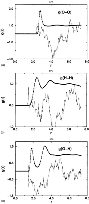
In Fig. 1, we present our results for the intermolecular rdfs of TIP4P water @g~O–O!(r), g~O–H!(r), and g~H–H!(r)]. In all cases an excellent agreement between RMC and MMC is shown, and the reversed calculations reproduce the rdfs within 0.1%–0.2%. Similar results were obtained with the SPC model and likewise for the flexible SPCFX and the experimental case, as shown in Figs. 2–4.

To the best of our knowledge such an essentially perfect agreement has not been reported before. In Figs. 1–4 the dashed lines represent the corresponding differences @g_ej(ri)2gj(ri)#3103. The order of deviations, 1022– 1023, is rather small and within statistical errors of a simulation. However, it is 102– 103 times larger than what has been ob-served for spherical Lennard-Jones particles.31,36

We stress again that in all RMC simulations in this re-port, the particles were allowed to approach at any distance, i.e., they were not prevented from overlapping. Nevertheless, no deviations were found in the short-range region, which is the case for most RMC simulations presented in the litera-ture. When a similar comparison, reported by Ref. 20, was made for the SPC model, the first peak for g~H–H! was sig-nificantly lower than the corresponding MC value. In the same report, RMC results obtained by fitting experimental data showed the common drawback of previous RMC ver-sions, and g~H–H!and g~O–O!exhibited sharp cutoffs at small separations instead of decreasing gradually to zero. Devia-tions around the first minimum of g~O–H! _{were also clearly} seen. We did not find any of those discrepancies.

It is also interesting to note that g~H–H! _{has smaller} de-viations than g~O–O!. The better g~H–H! statistics could to some extent be a trivial consequence of the fact that four times as many H–H pairs are available. Alternatively, these findings could follow from the associative properties of the liquid in the sense that strong hydrogen bonds are formed. This gives a special feature to the water structure and this information, hidden in the rdfs, could be more difficult to be fully reproduced in the RMC fitting. A revealing test would be to perform similar studies with other three-site molecules.

(5)

Liquid hydrogen sulphide would be an appropriate candi-date, since it is a molecule with large similarities to water and yet has less tendency to form hydrogen bonds. Such study is in progress.

As shown in Fig. 3 the largest deviations are observed for the flexible SPCFX model rdfs when reproduced by the RMC with a rigid geometry. Even though the rdfs are well fitted, the RMC finds difficulties arranging configurations of

rigid molecules to perfectly fit the structure generated by the flexible water model. One would expect similar differences when using real experimental data as the input for the RMC, as is, in fact, seen in Fig. 4.

In general, the agreement could be improved by decreas-ing the bin size~dr!. Discussions regarding the importance of

dr have already been given for spherical particles,31,36and it is sufficient to mention some basic aspects. RMC is unable to distinguish positions within the same bin, and within this resolution every point is equivalent. For this reason, layers

FIG. 1. Comparison between MMC~closed circles!and RMC~solid line!

radial distribution functions~rdfs!for the TIP4P water model. The dashed

line shows the difference @gMMC

j

(ri)2gMMC j

(ri)#3103: ~a! gO–O(r), ~b!

gH–H_{(r), and}_~_c_!_gO–H_(r).

FIG. 2. Comparison between MMC and RMC rdfs for SPC water. Notations are the same as in Fig. 1.

910 J. Chem. Phys., Vol. 114, No. 2, 8 January 2001 da Silvaet al.

(6)

between close contact and the first maximum will be overes-timated, while layers where the rdf is decreasing will be underestimated. This can be visualized by performing a RMC simulation with the same bin as the experimental one, and then calculating the rdf for the generated RMC configu-rations with a smaller grid on the analysis phase. With a large experimental grid size, an interpolation of experimental points in order to refine the data and generate appropriate input for RMC is recommended.

B. Hydrogen bond analysis

Liquid water has the peculiar characteristic of forming strong HB, which is manifested in the rdfs. In the literature, different definitions for HB are found based on geometric and/or energetic criteria.5 Generally, in RMC applications, where the pair interactions are unknown, only a geometrical criterion could be used. However, for our theoretical studies, the energetic form of Jorgensen et al. will be taken.6 With this definition, one assumes the existence of a hydrogen bond for any pair of molecules whenever they interact with an energy of at least 22.25 kcal/mol. After identifying a HB, the angles formed between the hydrogen donor ~f, O–H¯O!and acceptor~v, H¯O–H!are used to

character-ize the structure.6

Assuming that the particles interact according to the TIP4P model, we were able to calculate for instance the per-centage of molecules having nHBhydrogen bonds. It should

be stressed that the interaction potential was necessary only for the present analysis purposes.

FIG. 5. The angular distribution functions, P, as a function offand v.

Closed circles represent MMC data, while the solid line is the RMC result

with dr50.01 and the dashed line is the RMC result with dr50.05.

FIG. 3. MMC and RMC rdfs for the flexible water model SPCFX. Notations are the same as in Fig. 1.

FIG. 4. Comparison between experimental rdfs of real water~closed circles!

~from Ref. 41! and RMC rdfs. The dashed line shows the difference

@gEXP O–O

(ri)2gRMC O–O

(ri)#3103_.

(7)

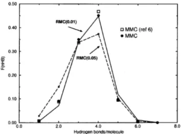
Figure 5 illustrates how the hydrogen bonds are oriented, while the percentage of clusters having n_HBhydrogen bonds is plotted in Fig. 6. In general, the RMC data were found to reproduce the MMC results well, particularly when a finer dr is used both for the input rdf and the RMC simulation.

As shown in Table I, the RMC average number of HB,

^

nHB

&

, and the average energy,

^

eHB

&

, are within the

statis-tical errors for dr50.01. It also seems that the hydrogen bond energy is not particularly sensitive to small structural changes. An analogous reasoning can be applied to the ori-entation formed by the hydrogen donor ~f, O–H¯O! and

acceptor~v, H¯O–H!as shown in Table I.

The agreement between RMC and MMC is surprisingly good, considering that the three-dimensional structure of a pair of water molecules depends on the Euler angles and the distance between the reference points of both molecules. These variables can be reduced to six ~five angles and the intermolecular distance!.42 _{As a consequence, the presented}

version of the RMC method, which used only three rdfs, i.e., three variables, could be working with an insufficient amount of information to fully reproduce the three-dimensional structure. Nevertheless, the hydrogen bond analysis shows that the main features of the structure are satisfactorily re-produced.

C. Configurational energy

The criterion of ‘‘goodness’’ for RMC results in terms of energetic analysis was introduced before.29,31,36,43 For many pair potentials, like Lennard-Jones, small changes in

the rdf may introduce large deviations in the configurational energy, U, since the dominant contributions come from small separations. For this reason, U is a sensitive indicator of the reliability of the RMC outcomes.

Table I shows the average energy of the present MMC and RMC simulations together with MC simulations of Jor-gensen et al.6 The RMC with small bin size satisfactorily reproduces the MMC energy, although the deviations are larger than one would expect from the excellent agreement found for the rdfs. The relative error is ;10 and 17% for

dr50.01 and dr50.05, respectively. When compared to Lennard-Jones studies,31,36 these numbers are at least five times larger. With the TIP4P model the O–O interaction dominates and it is exactly for this pair that we did find higher differences for the rdf.

Our results therefore indicate that even getting a near perfect agreement for all rdfs, as g~O–O!, g~H–H!, as

g~O–H! in liquid water, the three-dimensional structure of complex polyatomic molecules is not completely resolved by the RMC technique. The small angular distortions that we observed in Fig. 5, and also increased as the bin size in-creased, seem to be enough to produce the observed average energy discrepancies.

D. Sampling properties

Earlier RMC algorithms have suffered from sampling problems.32Therefore it is important to verify that indepen-dent configurations have been generated. To check this, one could for instance look at fluctuations of measurable thermo-dynamic variables or at the acceptance ratio. However, as we have also suggested,34 two complementary indicators of the sampling properties of the system should be used in a RMC simulation. It is convenient to follow the displacement of the particles and to characterize the physical state of the col-lected configurations by the order parameter Eq.~5!. Indeed, even the acceptance ratio should be analyzed in more detail, e.g., by looking to blocks of the production run.

In Fig. 7, the behavior of the acceptance ratio is shown as a function of the number of RMC cycles (N_cycles) at the production phase. The data is for the SPC-RMC system. Each point corresponds to a block average over 100 cycles. New configurations are accepted in this case with an almost constant probability of 23%. There is no indication that the method is sampling the same configuration during the obser-vation time. In contrast, new configurations have been gen-erated at a reasonable ratio. It still remains a question of how much the particles are moving, which can be seen from the

FIG. 6. The percentage of clusters with nHBhydrogen bonds. Notations are

the same as in Fig. 5.

TABLE I. Comparison of the average total configurational energy, U, and hyd0rogen bond properties for the TIP4P model, using two different ‘‘bin’’ sizes.^nHB&and^eHB&correspond to the average number of HB and

the average energy, respectively. The anglesfandvare defined as in the text.

Simulation Jorgensen MMC RMC2dr50.01 RMC2dr50.05

^U&~kcal/mol! 210.07 210.2060.14 29.1860.09 28.4660.08

^nHB& 3.57 3.5560.09 3.6460.07 3.3960.07 ^eHB&~kcal/mol! 24.17 24.1360.12 24.2360.08 24.2760.07

^v& ~deg! 99 99 98 98

^f& ~deg! 158 157 156 155

(8)

development of

^

Dr2

&

as a function of Ncycles. In Fig. 8 the

translational displacement of the oxygen atoms is plotted. It is evident from Fig. 8 that the particles are exposed to ratio-nal displacements and are not trapped into phase space points that could correspond to local minima. On the contrary, their displacement have similar behavior as found in ordinary MC simulations. Nevertheless, to certify that the system is really in the liquid state, the order parameter, O(t), defined in Eq. ~5!was also analyzed. In Fig. 9, a plot of O(t) as a function of RMC Ncycles is presented. The mean value of O(t) is 20.8, which is of the same order as the values reported by Berne and Harp for a Stockmayer fluid.39Similar behavior is found for other systems, e.g., the mean value of O(t) for EXPT-RMC was found to be 20.3 for a RMC simulation with an acceptance ratio of 17%. These values are character-istic for a system in the liquid state. However, we should point out that O(t) is also sensitive to the choice of transla-tional and rotatransla-tional displacement parameters. There is a

coupling between these parameters that does not seem to obey a general rule. The only trend already found is that decreasing the translational displacement parameter and in-creasing the rotational one usually leads to a bit higher ac-ceptance and translational ‘‘diffusion coefficients’’~the slope of the graphic

^

Dr2

&

as a function of the Ncycles). A more

systematic and strictly technical study will be addressed in forthcoming works.

V. CONCLUSIONS

RMC is a novel molecular modeling technique, still un-der development. One basic problem, the complete reproduc-tion of the input rdfs, was eliminated with the algorithm proposed in this paper. The liquid water structure was suc-cessfully reproduced without any ad hoc constraints, even when real experimental data were used as the input. With the studied algorithm it is sufficient to have a small number of particles~of the order of 100!.

The average energy may be sensitive to small configu-rational changes. This fact increases the demands on the RMC technique to generate adequate configurations. The simulation tests presented in this report indicate that the new algorithm is successful in this respect, at least with a bin size small enough. Also the hydrogen bond analysis showed quite good agreement between the RMC results and the MC simu-lations.

On the other hand, we have also seen that an excellent reproduction of the input rdfs, although necessary, is not sufficient to guarantee prediction with the same accuracy for other properties in a polyatomic liquid such as water. This is probably a consequence of the fact that it is not enough to consider only three input variables, namely the available rdfs. However, to neglect small angular corrections seems not to severely affect for instance the configurational energy. This finding opens up new perspectives for RMC studies of molecular liquids. The present study might be extended to extract fairly accurate angular correlations from experimental water data and to improve existing water pair potentials. This

FIG. 7. The acceptance ratio during the production phase as a function of

the number of RMC cycles (Ncycles). Each point in the graph corresponds to

an average over 100 RMC cycles. Data are obtained for the SPC-RMC system.

FIG. 8. The mean square translational displacement (^Dr2_&_{) of oxygen}

atoms in units of Å2as a function of the RMC simulation cycles (Ncycles).

The data are obtained for the SPC-RMC system and collected during the production phase.

FIG. 9. Translational order parameter @O(t)# for the oxygen atoms as a

function of the RMC simulation cycles (Ncycles). The system and conditions

are the same as in Fig. 8.

(9)

work has already been started and the results will be pre-sented in a forthcoming paper.

ACKNOWLEDGMENTS

This work was supported in part by the Conselho Nacio-nal de Desenvolvimento Cientı´fico e Tecnolo´gico, by the Fundaçaõ de Amparo a` Pesquisa do Estado de Saõ Paulo, and Grant No. G-970000741 from CONICIT-Venezuela. We are also grateful to Professor Bo Jo¨nsson for makingMUMOD available to us. W.O.R. acknowledges CONACYT-Me´xico for the Catedra Patrimonial de Excelencia granted.

1_{N. A. Metropolis, A. W. Rosenbluth, M. N. Rosenbluth, A. Teller, and E.}

Teller, J. Chem. Phys. 21, 1087~1953!.

2_{M. P. Allen and D. J. Tildesley, Computer Simulation of Liquids}_~_Oxford

University Press, Oxford, 1989!.

3_{D. Frenkel and B. Smit, Understanding Molecular Simulation: From} Al-gorithms to Applications~Academic, San Diego, 1996!.

4_{J. A. Barker and R. O. Watts, Chem. Phys. Lett. 3, 144}_~₁₉₆₉_!_. 5_{B. M. Ladanyi and M. S. Skaf, Annu. Rev. Phys. Chem. 44, 335}_~₁₉₉₃_!_. 6

W. L. Jorgensen, J. Chandrasekhar, J. D. Madura, R. W. Impey, and M. L. Klein, J. Chem. Phys. 79, 926~1983!.

7_{O. Teleman, B. Jo¨nsson, and S. Engstro¨m, Mol. Phys. 60, 193}_~₁₉₈₇_!_. 8_{W. L. Jorgensen, J. Chem. Phys. 77, 4156}_~₁₉₈₂_!_.

9

H. J. C. Berendsen, J. P. M. Postma, W. F. van Gunsteren, and J. Her-mans, in Intermolecular Forces, edited by B. Pullman~Reidel, Dordrecht, 1981!, pp. 331–342.

10_{L. Blum and L. Degre`ve, Mol. Phys. 88, 585}_~₁₉₉₆_!_.

11_{L. Blum, F. Vericat, and L. Degre`ve, Physica A 265, 369}_~₁₉₉₉_!_. 12

M. Levitt, Chem. Scr. 29A, 197~1989!.

13_{S. Zhu, S. Singh, and G. W. Robinson, Adv. Chem. Phys. LXXXV, 627}

~1994!.

14_{R. Kaplow, T. A. Rowe, and B. L. Averbach, Phys. Rev. 168, 1068}

~1968!.

15

R. L. McGreevy and L. Pusztai, Mol. Simul. 1, 359~1988!.

16_{R. L. McGreevy and M. A. Howe, Phys. Chem. Liq. 24, 1}_~₁₉₉₁_!_. 17_{R. L. McGreevy and M. A. Howe, Annu. Rev. Mater. Sci. 22, 217}_~₁₉₉₂_!_. 18_{F. L. B. da Silva, A. R. de Souza, C. Quintale, Jr., and L. Degre`ve, XVI}

Conference on Condensed Matter Physics, Caxambu´, Brazil, 1993, p. 156.

19_{P. Jedlovszky, I. Bako´, and G. Pa´linka´s, Chem. Phys. Lett. 221, 183}

~1994!.

20_{P. Jedlovszky, I. Bako´, G. Pa´linka´s, T. Radnai, and A. K. Soper, J. Chem.}

Phys. 105, 245~1996!.

21_{A. K. Soper, Chem. Phys. 202, 295}_~₁₉₉₆_!_. 22

H. Xu and M. Kotbi, Chem. Phys. Lett. 248, 89~1996!.

23_{P. Jedlovszky and R. Vallauri, J. Chem. Phys. 105, 2391}_~₁₉₉₆_!_. 24

R. L. McGreevy, J. Phys.: Condens. Matter 3, f9~1991!.

25_{C. Andreani, M. A. Ricci, M. Nardone, F. P. Ricci, and A. K. Soper, J.}

Chem. Phys. 107, 214~1997!.

26_{M. Ostheimer and H. Bertagnolli, Mol. Simul. 3, 227}_~₁₉₈₉_!_. 27

A. P. Lyubartsev and A. Laaksonen, Phys. Rev. E 52, 3730~1995!.

28_{A. Shick and R. Rajagopalan, Colloids Surface 66, 113}_~₁₉₉₂_!_. 29

G. To´th and A. Baranyai, J. Chem. Phys. 107, 7402~1997!.

30_{J. H. Finney, Faraday Discuss. 103, 1}_~₁₉₉₆_!_. 31

F. L. B. da Silva, B. Svensson, T. A˚ kesson, and B. Jo¨nsson, J. Chem. Phys. 109, 2624~1998!.

32

See discussions at Faraday Discuss. Faraday Discuss. 103, 106~1996!.

33_{G. To´th, L. Pusztai, and A. Baranyai, J. Chem. Phys. 111, 5620}_~₁₉₉₉_!_. 34_{F. L. B. da Silva, B. Svensson, T. A}_{˚ kesson, and B. Jo¨nsson, J. Chem.}

Phys. 111, 5622~1999!.

35_{R. L. McGreevy, M. A. Howe, and J. D. Wicks, RMCA—A general} pur-pose Reverse Monte Carlo Code~Manual, 1993!.

36_{W. Olivares-Rivas, F. L. B. da Silva, and L. Degre`ve}_~_unpublished_!_. 37_{F. L. B. da Silva, A. R. de Souza, and L. Degre`ve, XX Conference on}

Condensed Matter Physics, Caxambu´, Brazil, 1997, p. 106.

38_{R. Evans, Mol. Simul. 4, 409}_~₁₉₉₀_!_.

39_{B. J. Berne and G. D. Harp, Adv. Chem. Phys. XVII, 63}_~₁₉₇₀_!_. 40_{O. Teleman and B. Jo¨nsson, J. Comput. Phys. 7, 58}_~₁₉₈₆_!_. 41_{A. K. Soper and M. G. Philips, Chem. Phys. 107, 47}_~₁₉₈₆_!_. 42

L. Degre`ve, V. M. de Pauli, and M. A. Duarte, J. Chem. Phys. 106, 655

~1997!.

43_{F. L. B. da Silva and L. Degre`ve, Annals of 11th Nordic Symposium on}

Computer Simulations, Hillerød, 1997, p. 34.