PLEASE SCROLL DOWN FOR ARTICLE
On: 24 April 2009Access details: Access Details: [subscription number 910710910] Publisher Taylor & Francis
Informa Ltd Registered in England and Wales Registered Number: 1072954 Registered office: Mortimer House, 37-41 Mortimer Street, London W1T 3JH, UK
Sequential Analysis
Publication details, including instructions for authors and subscription information:
http://www.informaworld.com/smpp/title~content=t713597296
Power of the Sequential Monte Carlo Test
I. Silva a; R. Assunção a; M. Costa aa Departamento de Estatística, Universidade Federal de Minas Gerais, Belo Horizonte, Minas Gerais, Brazil
Online Publication Date: 01 April 2009
To cite this Article Silva, I., Assunção, R. and Costa, M.(2009)'Power of the Sequential Monte Carlo Test',Sequential Analysis,28:2,163 — 174
To link to this Article: DOI: 10.1080/07474940902816601 URL: http://dx.doi.org/10.1080/07474940902816601
Full terms and conditions of use: http://www.informaworld.com/terms-and-conditions-of-access.pdf This article may be used for research, teaching and private study purposes. Any substantial or systematic reproduction, re-distribution, re-selling, loan or sub-licensing, systematic supply or distribution in any form to anyone is expressly forbidden.
Copyright © Taylor & Francis Group, LLC ISSN: 0747-4946 print/1532-4176 online DOI: 10.1080/07474940902816601
Power of the Sequential Monte Carlo Test
I. Silva, R. Assunção, and M. Costa
Departamento de Estatística, Universidade Federal de Minas Gerais, Belo Horizonte, Minas Gerais, Brazil
Abstract: Many statistical tests obtain theirp-value from a Monte Carlo sample ofmvalues of the test statistic under the null hypothesis. The numbermof simulations is fixed by the researcher prior to any analysis. In contrast, the sequential Monte Carlo test does not fix the number of simulations in advance. It keeps simulating the test statistics until it decides to stop based on a certain rule. The final number of simulations is a random numberN. This sequential Monte Carlo procedure can decrease substantially the execution time in order to reach a decision. This paper has two aims concerning the sequential Monte Carlo tests: to minimize N without affecting its power; and to compare its power with that of the fixed-sample Monte Carlo test. We show that the power of the sequential Monte Carlo test is constant after a certain number of simulations and therefore, that there is a bound toN. We also show that the sequential test is always preferable to a fixed-sample test. That is, for every test with a fixed sample sizemthere is a sequential Monte Carlo test with equal power but with smaller number of simulations.
Keywords: Monte Carlo test; p-value; Sequential estimation; Sequential test; Significance test.
Subject Classifications: 62L05; 62L15; 65C05.
1. INTRODUCTION
To carry out hypothesis testing, one must find the distribution of the test statistic
U under the null hypothesis, from which thep-value is calculated. Either because it
Received April 15, 2008, Revised February 1, 2009, February 5, 2009, Accepted February 8, 2009
Recommended by Nitis Mukhopadhyay
Address correspondence to I. Silva, Departamento de Estatística, Universidade Federal de Minas Gerais, Avenida Presıdente Antonio Carlos, 6627, Prédio do ICEx, Sala 4054, Pampulha, Belo Horizonte, Minas Gerais 31270-901, Brazil; Fax: 55-31-3409-5924; E-mail: [email protected]
is too cumbersome or it is impossible to obtain this distribution analytically, Monte Carlo tests are used in many situations (Manly, 2006). In particular, areas such as spatial statistics (Assunção et al., 2007; Diggle et al., 2005; Kulldorff, 2001) and data mining (Kulldorff et al., 2003; Rolka et al., 2007) rely heavily on Monte Carlo tests to draw inference. Other areas have situations in which Monte Carlo tests seems to be the best current approach, such as the exact tests in categorical data analysis (Booth and Butler, 1999; Caffo and Booth, 2003), and some regression problems in econometrics (Khalaf and Kichian, 2005; Luger, 2006).
The conventional Monte Carlo test generates a large number of independent copies ofU from the null distribution. Assuming that large values ofU lead to the null hypothesis rejection, a Monte Carlo value is calculated based on the proportion of the simulated values that are larger or equal than the observed value ofU.
As the statistics field evolves to deal with ever more complex models, Monte Carlo tests become costly. The simulation of each independent copy ofU under the null hypothesis can take a long time.
In many applications, after a few simulations are carried out, it becomes intuitively clear that a large number of simulations is not necessary. For instance, suppose that after 100 simulations, the observed value is around the median of the generated values. It is not likely that the null hypothesis will be eventually rejected even if a much larger number of simulations (such as 9999) is carried out. Most researchers would be confident to stop at this point if a valid p-value could be provided.
Besag and Clifford (1991) introduced the idea of sequential Monte Carlo tests, an alternative way to obtain p-values without fixing the number of simulations previously. Their method makes a decision concerning the null hypothesis after each simulated value up to a maximum number of simulations. This approach can substantially shorten the number of simulations required to decide about the significance of the observed test statistic.
Although the proposal of Besag and Clifford (1991) stands as a major contribution to the practice of modern data analysis, it is under utilized and has some unanswered theoretical questions. One important aspect of the sequential Monte Carlo tests is the relative comparison of its power with that of the conventional Monte Carlo test. Based on the Besag and Clifford results, we can always obtain a sequential Monte Carlo with significance level that does not require more simulations than a conventional Monte Carlo test at the same level. However, the relationship between the power functions of these tests is not clear. In terms of power, is there a cost when we apply the sequential test instead of the conventional Monte Carlo test? The answer is no, and the first aim of this paper is to demonstrate this. The second objective of this work is to show how we can make the choice of the maximum number of simulations in the sequential Monte Carlo tests without losing power.
The next section contains a summary of the definitions and notation associated with the conventional and the sequential Monte Carlo tests. Section 3 discusses the power of the sequential procedure and Section 4 shows how to establish the parameters of the sequential test such that it has the same power as a given conventional Monte Carlo test. In Section 5, we develop bounds for the difference of power between a conventional and a sequential Monte Carlo tests. Section 6 closes the paper with a discussion of the implications of our results.
2. A SEQUENTIAL MONTE CARLO TEST
Let U be a test statistic with distributionF under the null hypothesisH0. Suppose that large values ofU leads to the rejection of the null hypothesis. WhenF can be evaluated explicitly, thep-value of the upper-tail test based on the observed valueu0
ofU is given byp=1−Fu0. LetP=1−FUbe the random variable associated with the p-value. If F is a continuous function, P has a uniform distribution in
01under the null hypothesis. When we can not evaluateFwe need to find other ways to calculate the p-value. The Monte Carlo test proposed by Dwass (1957) is an alternative if we can simulate samples from the null hypothesis.
The fixed-size or conventional Monte Carlo test generates a sample of size
m−1 of the test statistic U under the null hypothesis H0. Denote each simulated value by ui,i=1 m−1. The Monte Carlo p-value pmc is equal to r/m if the observed value u0 is the rth largest value among the mvalues u0 u1 um−1. In
this conventional Monte Carlo procedure, if the rank ofu0 is among them larger ranks ofu0 u1 um−1, we reject the null hypothesis at thesignificance level. We
denote this procedure byMCconvm .
Let Pmc be the corresponding random variable associated with the realized Monte Carlo p-valuepmc. Under the null hypothesis, we havePmc≤a=a ifa is one of the values 1/m2/m 1. That is, the Monte Carlo p-value Pmc has a uniform distribution on the discrete set 1/m2/m 1. Let W be the random variableW =Pmc−XwhereX∼U01/mand it is independent ofPmc. Then,W ∼ U01under the null hypothesis. In this sense, Besag and Clifford (1991) say that the Monte Carlo p-value is exact, because Pmc has the same uniform distribution under the null hypothesis than the analyticalp-value P=1−FU. In addition to that, irrespective of the validity of the null hypothesis,Pmc →P almost everywhere because, for any observed valueu0, we have
pmc=
1+#ui≥u0
m =
1
m+
#
ui≥u0
m−1
m−1
m →1−Fu0
asmgoes to infinity.
However, when early on there is little evidence against the null hypothesis, it is wasteful to run the procedure for large values ofmsuch as, for example,m=10000. This is the main motivation for Besag and Clifford to develop the sequential Monte Carlo test. In brief, the sequential version of the test selects a small integerh, such ash=10 orh=20. It keeps simulating by Monte Carlo from the null hypothesis distribution until h of the simulated values are larger than the observed value u0. There is also an upper limitn−1 for the total number of simulations. Thep-value is based on the proportion of simulated values larger thanu0at the stopping time.
In other words, simulate independently and sequentially the random values
U1 U2 UL from the same distribution as U under the null hypothesis. The random variable L has possible values h h+1 n−1 and its value is determined in the following way:Lis the first time when there arehsimulated values larger thanu0. If this has not occurred at step n−1, then let L=n−1. Let g be the number of simulated Ui’s larger than u0 at termination. If we denote byl the
realized number of Monte Carlo withdrawals, then the sequentialp-value is given by
ps=
h/l ifg=h
g+1/n ifg < h (2.1)
For example, if up ton−1=999 Monte Carlo withdrawals are considered and the sampling scheme stops as soon as h=10 exceeding values of U occurs, then the possible values of the sequentialp-value are 10/10, 10/11, 10/12 10/1000, 9/1000, 8/1000 1/1000. Note that the support of the sequential Monte Carlo procedure is more concentrated on the lower end of the interval 01. This is a desirable characteristic because these are the p-value possible values that we want to know more precisely.
Let the support ofps be denoted by
S=1/n2/n h/n h/n−1 h/h+2 h/h+11
The values of the form h−q/n, with 0≤q≤h−1, occur when we need to run the procedure up to the maximum n−1 number of simulations without never getting h uis larger thanu. The other values, of the formh/h+q, with h≤h+ q≤n−1, occur when we either stop the procedure earlier than the maximumn−1 or when the hth larger value occur exactly at the n−1th sequential observation and hencel=n−1. Therefore, we can also define the sequentialp-value as
ps=
h/l ifl < n−1
h/l ifl=n−1 andg=h g+1/l+1 ifl=n−1 andg < h
Ifa∈S, thenPs≤a=aunder the null hypothesis. To see this, assume that a=h/h+q≤1 with h≤h+q < n. Then
Ps≤a=Ps≤h/h+q=L≥h+q
=L > h+q−1= h
h+q
because L > h+q−1 if, and only if, after l−1 Monte Carlo withdrawals, the observed u is among the largest h of the sample of equally probable l−1+1 elements. Consider now thata=h−q/nwith 0≤q≤h−1. Then
Ps≤a=Ps≤h−q/n
=L=n−1 and onlyh−q−1 exceedingu
=uis theh−qth largest amongn
=h−q/n
We can transform Ps by subtracting a random variable X such that the sequential
p-value also has a continuous uniform distribution in 01. For that, define
X conditionally on the observed value of the discrete p-value Ps Suppose that ps=b∈S. Let a be the largest element of S that is smaller than b Define a=0 ifb=1/n. ThenX∼Ua bandPs−X has a uniform distribution in01under the null hypothesis, exactly as thep-valuesPandPmc. Because this is less common to be carried out in practice, in the remaining of this paper we will not transform
Ps in this way, keeping its definition as in (2.1).
The most important random variable in our paper is L, the total number of simulations carried out, which has distribution under the null hypothesis given by
L≤l=
0 sel≤h−1
1−h/l+1 sel=h h+1 n−1
1 ifl=n
Its expected value was found by Besag and Clifford (1991):
L= n−1
l=1
PL≥l= n−1
l=h+1
l−1h+hlog n−05
h+05
(2.2)
To reach a decision with the sequential Monte Carlo test, it is necessary to fix the values of three tuning parameters, n h, and , and hence we denote the test byMCseqn h . Typically, nis taken equal to the number mof simulations one would run if carrying out the conventional Monte Carlo test. Whether this typical choice is really necessary is one of the issues studied in this paper.
3. POWER OF THE SEQUENTIAL MONTE CARLO TEST
In this section we study the power of the sequential Monte Carlo procedure
MCseqn h . Its behavior depends on the value ofnwith respect toh/+1. We deal initially with the casen≥h/+1.
3.1. MCseqn h with n≥h/+1
This constraint implies that≥h/n−1. That is, is not smaller than h divided by the maximum number of simulations. A typical choice found in practical analysis isn−1=999 and=005. Then, the conditionn≥h/+1 is valid ifh≤49. This is likely to cover most of the choices one would make forhin practice.
The power of the procedureMCseqn h is constant for alln≥h/+1 and hence, takingnlarger thanh/+1 is not worth in terms of power. In other words,
n= h/ +1 is optimal in terms of number of simulations for a test with error type I probability. The notationxrepresents the ceiling ofxthe smallest integer greater or equal tox
To see this result, label the eventUi≥u0 as a success. BecauseUihas c.d.fF the probabilityUi≥u0is the observedp-valuep=1−Fu0. The probability of
carrying outLsimulations untilhsuccesses is given by:
L=l P=p=
l−1
h−1
ph1−pl−h ifl=h h+1 n−2
x=n−1
x−1
h−1
ph1−px−h ifl=n−1
We reject H0 if, and only if, h/≤L≤n−1. This means that in h/ −1 simulations, we obtain at mosth−1 successes. Therefore, for an observed valueu0, the probability of rejectingH0 in the sequential test is given by
RejectH0 P=p=L≥h/ P =p
=L > h/−1 P=p
= h−1
x=0
h/−1
x
px1−ph/−x−1 (3.1)
Because the last expression does not involve n, the power of the sequential Monte Carlo test is constant as long as n≥h/+1. Because the error type I is fixed at,h/ +1 is an upper bound forn.
For example, ifh=5 and=005, thenn=101 minimize the sampling effort while holding constant the test power. It is not worth to select a larger sample size such as, for examplen=1000, expecting to have a better test. Using (2.2), we know that L≈19 if n=101 under the null hypothesis. If one decides to use
n=1000, then L≈31, 50% larger compared with that associated with optimal
n However, the more substantial gain of using the optimal n is when the null hypothesis is false. In this situation, it is more probable that we need to run the sequential test up to the maximum numbern−1 of simulations and then choosing
n=101 will save many simulations compared with the larger sample sizen=1000, which does not increase the power.
3.2. MCseqn h withn < h/+1
The power of the procedureMCseqn h do not have a monotone behavior with the increase of n when it is in the range h+1< n < h/+1. In fact, at least in principle, the power can have a non-monotone behavior as n increases from h+ 1 towards the h/+1. However, the most usual behavior is that the power is an increasing function ofnfornin that range.
To understand this limitation of the analysis, let us assume that n < h/+1. We have two possible evaluations of the sequentialp-value depending on the value ofgaccording to (2.1). Hence, we reject the null hypothesis either when estimating thep-value by g/lor when estimating thep-value by g+1/n.
However, we can never reject the null hypothesis if thep-valuepsis of the form
g/l The reason is that, if ps=g/l then we obtained h values exceeding u The smallest value for g/lish/n−1. Becausen < h/+1, we have thatps≥h/n− 1 > and we can not reject the null hypothesis.
Therefore, the only other possibility to reject the null hypothesis when n < h/+1 is whenps is of the formg+1/n. In this case, we needg+1/n≤, or g≤n−1. Given thatP=pthe probability of rejectingH0 is equal to
G≤n−1 P=p=
n−1
x=0
n−1
x
px1−pn−1−x (3.2)
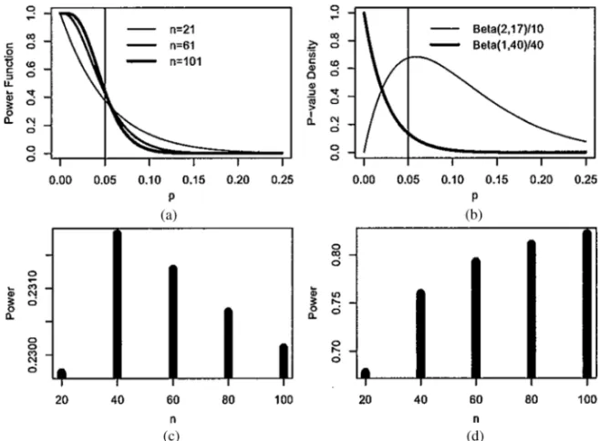
Figure 1(a) shows the shape ofG≤n−1 P=p for=005,h=5, andn= 2161101. The power forn < h/+1 is given by integrating out (3.2) with respect
Figure 1. Power behavior of the sequential Monte Carlo test and thep-value density.
to thep-value probability distributionFp:
n h FP= 1
0
G≤n−1 P=pFPdp
=
1
0 n−1
x=0
n−1
x
px1−pn−1−xFPdp (3.3)
Denote by n h FP the power function of the sequential procedure. Depending onFP, the power curve can be non-monotone. To illustrate this result, consider two differentFP distributions. One of them assumes thatP is distributed according to a Beta distribution with parameters 2 and 17. The other assumes a Beta distribution with parameters 1 and 40 (see Figure 1(b)). The graph in Figure 1(c) shows the power (3.3) usingFP as a Beta217 distribution withh=5, =005, andn=20, 40, 60, 80, 100. We can see that the power does not increase withnin the range 61≤n≤101.
In contrast, Figure 1(d) shows the power usingFP∼Beta140and the same tuning parameters as before. In this case, the power is increasing with n. Indeed, Hope (1968) and Jockel (1986) showed that we always have the power increasing with n if thep-value distribution FP belongs to certain distribution classes, which include the Beta140distribution.
This illustrative example shows that, for n < h/+1, the sequential power behavior depends heavily on the shape of thep-value density.
4. A SEQUENTIAL MC TEST EQUIVALENT TO A FIXED-SIZE MC TEST
From now on, we consider only the casen≥h/+1. Given a conventional Monte Carlo test MCconvm , we find in this section a sequential test MCseqn h
with the same power as the conventional one. For the fixed-size Monte Carlo test, letGbe the random count ofUis that are greater or equal to u0 among them−1
generated. The null hypothesis is rejected ifG+1/m≤or, equivalently, if G≤
m−1. The random variableGhas a binomial distribution with parametersm−1 and success probability equal to thep-valuePTherefore,MCconvm rejects the null hypothesis with probability
RejectH0 P=p=PG≤ m −1 P=p
=
m−1
y=0
m−1
y
py1−pm−y−1 (4.1)
TheMCconvm power is
m FP=
1
0 m−1
y=0
m−1
y
py1−pm−y−1F
Ppdp (4.2)
whereas the MCseqn h power forn > h/+1 is given by integrating out (3.1) with respect to FP:
n h FP= 1
0
h−1
x=0
h/−1
x
px1−ph/−x−1F
Ppdp (4.3)
As a result, the power (4.3) of MCseqn h and the power (4.2) of
MCconvm are equal if we take h=m. That is, given a conventional MC procedure MCconvm , we have sequential MC procedure in MCseqn m
with equal power. This is valid for alln > h/+1 and hence we take the minimum possible value n= h/ +1 to have the equivalent proceduresMCconvm and
MCseqm+1 m .
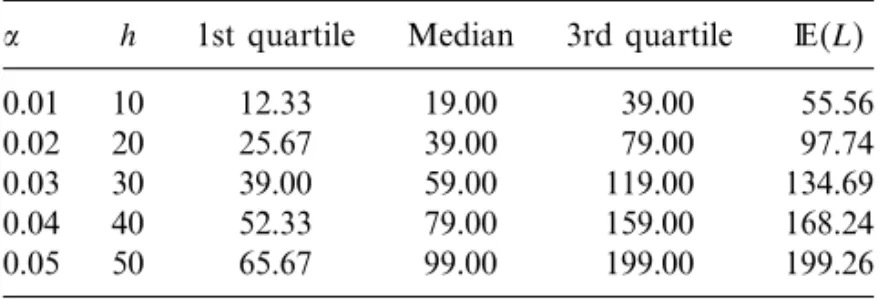
Under the null hypothesis or under an alternative not too far from the null, there will be considerable reduction in the number of simulations required to reach a decision if the sequential test is adopted holding fixed the main statistical characteristic (size and power) of the fixed-size MC tests. Table 1 shows the quartiles of the null distribution of L for the sequential MC test MCseqm+1 m
equivalent to the conventional MC test MCconvm with different significance levelbetween 0.01 and 0.05, and withm=1000 andn=1001. Therefore, we can have large gains if the sequential procedure is adopted.
We showed that, given a conventional MC test, there is a simple rule to find a sequential MC test with the same power but typically requiring a smaller number of simulations. However, one can trade a slight power loss in exchange for a smaller number of Monte Carlo simulations. If we want to adopt a general sequential MC test rather than the fixed-size MC test, it is important to have control over the power loss we are subjected. The next section establishes bounds for this loss.
Table 1. Quartiles of the null distribution of L for some sequential MC test equivalent to the conventional MC test with m=h/
h 1st quartile Median 3rd quartile L
0.01 10 12.33 19.00 39.00 55.56
0.02 20 25.67 39.00 79.00 97.74
0.03 30 39.00 59.00 119.00 134.69
0.04 40 52.33 79.00 159.00 168.24
0.05 50 65.67 99.00 199.00 199.26
5. BOUNDS ON THE POWER DIFFERENCES
Equations (3.1) and (4.1) give the null hypothesis rejection probability for
MCseqn h and MCconvm for a fixed realized p-value P=p. Because it is wasteful to takenlarger than h/+1, we assume thatn is equal toh/ +1. To obtain the power, we need to integrate (3.1) and (4.1) with respect to the probability density fPp of P. Under the null hypothesis,fPp is the density of an uniform distribution in01. Under an alternative hypothesis,fPpis concentrated towards the lower half of the interval01.
LetDPbe the random variable
DP= m−1
y=0
m−1
y
Py1−Pm−y−1− h−1
x=0
h/2 −1
x
Px1−Ph/2−x−1
(5.1)
The power difference betweenMCconvm andMCseqh/ +1 h is given by
EDP =
1
0
DPfPpdp (5.2)
A crude bound for the difference in power is obtained by finding real numbersa
andbsuch that a≤DP≤b. Letbm h 2be the upper bound for the power difference between MCconvm and MCseqh/2 +1 h 2, respectively. Note that we can obtain crude bounds for=2.
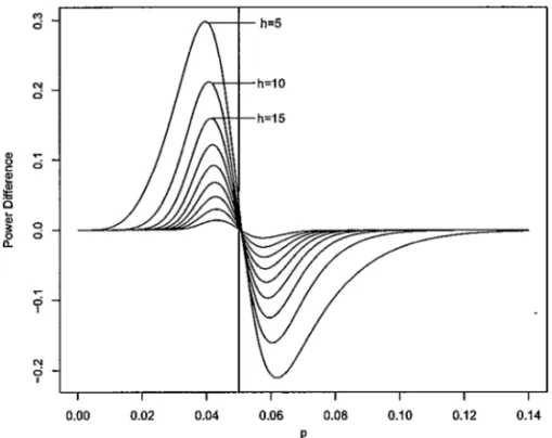
Figure 2 shows a graph of the power difference Dp between
MCconv1000005 and MCseqh/005 +1 h005. Each curve p Dp
represents Dp for a given value of h, withh=510 45. The curve showing both the highest peak and deepest valley corresponds toh=5. As hincreases, the curves dampen and have less pronounced extreme values. Hence, the larger the value ofh, the smallerDp
For h=25, Dp assumes its maximum value when p≈00423, and the minimum when p≈00586. The maximum value of Dp is equal 0.0921, and it is a crude bound for the power difference between MCconv1000005
and MCseq50125005. This is so because Dp varies from its maximum (and positive) value to its minimum (and negative) value within a short interval in p. Because the powerEDp simply integratesDpwith respect tofPp, the extreme
Figure 2. Graph of the power difference function between the fixed-size and the sequential Monte Carlo tests.
value of Dp will be approximately the value of 0.0921 only if the densityfPp is tightly concentrated around the point of maximum. This is not likely to happen in practice and hence we can expect a much lower value for the powerEDp
Table 2 shows the values of the crude bound maxpDp=bm h for the power difference betweenMCconvm andMCseqn h withm=100010000,
=005 and h=515 500. We set n= h/ +1 in all cases. The fourth column shows these bounds form=1000 andm=10000 separately. The numbers in this column are also the power difference bounds between two conventional Monte Carlo tests, namely betweenMCconvm005andMCconvm2005, where
m2is shown in the third column.
For small h the crude bound is too large. However, this bound decreases quickly with h For example, when h=25, the MCseq50125005 has power smaller than MCconv1000005 by, at most, 0.09. For m=10000, the bound maxpDp decreases even faster.
Table 2. Crude bound maxpDp=bm h
m=1000 m=10000
h n m2 maxpDp h n m2 maxpDp
5 101 100 0.2980 100 2001 2000 0.1931
15 301 300 0.1595 150 3001 3000 0.1469
25 501 500 0.0921 250 5001 5000 0.0858
40 801 800 0.0296 400 8001 5000 0.0278
50 1001 1000 0.0000 500 7001 7000 0.0000
6. DISCUSSION AND CONCLUSIONS
The sequential Monte Carlo test is a feasible and more economical way to reach decisions in a hypothesis testing under Monte Carlo sampling. We have shown that for each conventional Monte Carlo test with m simulations, there is a sequential Monte Carlo procedure with the same significance level and power. More important, this sequential Monte Carlo test requires at most one additional simulation and its expected number of simulations is generally much smaller thanm, specially when the null hypothesis is true.
If execution time is crucial, the user can trade a small amount of power in the sequential test by a large decrease in number of simulations. To guide this trade-off choice, we develop bounds for the difference in power between theMCconvand
MCseqtests. This is more relevant if we consider that the true differences are likely to be much smaller than the bounds suggest. These bounds can also be used to compare two conventional Monte Carlo tests.
For n≥h/+1, an usual situation, the sequential MC test has a constant power and this leads to the suggestion of adoptingn=h/+1.
ACKNOWLEDGMENTS
The authors are grateful to Martin Kulldorff for very useful comments and suggestions on an earlier draft of this paper. This research was partially funded by the National Cancer Institute, grant number R01CA095979, Martin Kulldorff PI. The second author was partially supported by the Conselho Nacional de Desenvolvimento Científico e Tecnológico (CNPq). This research was partially carried out while the first author was at the Department of Ambulatory Care and Prevention, Harvard Medical School, whose support is gratefully acknowledged.
REFERENCES
Assunção, R., Tavares, A. I., Correa, T., and Kulldorff, M. (2007). Space-Time Cluster Identification in Point Processes,Canadian Journal of Statistics35: 9–25.
Besag, J. and Clifford, P. (1991). Sequential Monte Carlop-Values,Biometrika78: 301–304. Booth, J. G. and Butler, R. W. (1999). An Importance Sampling Algorithm for Exact
Conditional Tests in Log-Linear Models,Biometrika86: 321–332.
Caffo, B. S. and Booth, J. G. (2003). Monte Carlo Conditional Inference for Log-Linear and Logistic Models: A Survey of Current Methodology,Statistical Methods in Medical Research12: 109–123.
Diggle, P. J., Zheng, P., and Durr, P. A. (2005). Non-Parametric Estimation of Spatial Segregation in a Multivariate Point Process: Bovine Tuberculosis in Cornwall, UK, Journal of Royal Statistical Society, Series C54: 645–658.
Dwass, M. (1957). Modified Randomization Tests for Nonparametric Hypotheses,Annals of Mathematical Statistics28: 181–187.
Hope, A. C. A. (1968). A Simplified Monte Carlo Significance Test Procedure,Journal of Royal Statistical Society, Series B30: 582–598.
Jockel, K.-H. (1986). Finite Sample Properties and Asymptotic Efficiency of Monte Carlo Tests,Annals of Statistics14: 336–347.
Khalaf, L. and Kichian, M. (2005). Exact Tests of the Stability of the Phillips Curve: The Canadian Case,Computational Statistics & Data Analysis49: 445–460.
Kulldorff, M. (2001). Prospective Time Periodic Geographical Disease Surveillance Using a Scan Statistic,Journal of Royal Statistical Society, Series A164: 61–72.
Kulldorff, M., Fang, Z., and Walsh, S. J. (2003). A Tree-Based Scan Statistic for Database Disease Surveillance,Biometrics 59: 323–331.
Luger, R. (2006). Exact Perrmutation Tests for Non-Nested Non-Linear Regression Models, Journal of Econometrics133: 513–529.
Manly, B. F. J. (2006).Randomization, Bootstrap and Monte Carlo Methods in Biology, 3rd ed., Boca Raton: Chapman & Hall/CRC.
Marriott, F. H. C. (1979). Bernard’s Monte Carlo Test: How Many Simulations? Applied Statististics28: 75–77.
Rolka, R., Burkom, H., Cooper, G. F., Kulldorff, M., Madigan, D., and Wong, W. (2007). Issues in Applied Statistics for Public Health Bioterrorism Surveillance Using Multiple Data Streams: Research Needs,Statistics in Medicine26: 1834–1856.