A Novel Nonparametric Multiple Imputation Algorithm for Estimating Missing Data

(1)

Abstract— The treatment of incomplete data is an important step in pre-processing data prior to later analysis. We propose a novel non-parametric multiple imputation algorithm for estimating missing value. The proposed algorithm is based on Generalized Regression Neural Networks. We compare the proposed algorithm against existing algorithms on forty-five real and synthetic datasets. The effectiveness of imputation algorithms is evaluated in classification problems. The performance of proposed algorithm appears to be superior to that of other algorithms.

Index Terms—Missing values, imputation, single imputation, multiple imputation.

I. INTRODUCTION

Missing data is a common feature of real world datasets. By an incomplete or missing dataset we mean a dataset where, for some cases, the values of one or more explanatory variables are missing. Most data mining algorithms cannot work directly with incomplete datasets. Hence, missing value imputation is widely used for the treatment of missing values. A major focus of research today is to develop an imputation algorithm that preserves the multivariate joint distribution of input and output variables. Much of the information in these joint distributions can be described in terms of means, variances and covariances. If the joint distributions of the variables are multivariate normal, then the first and second moments completely determine the distributions.

The practice of filling in a missing value with a single replacement is called single imputation (SI) method. A major problem with SI is that this approach cannot reflect sampling and imputation uncertainty about the actual value. Rubin (1978) proposed multiple-imputation (MI) to solve this problem [1]. MI replaces each missing value in a dataset with

m

>

1 (where

m is typically small, e.g. 3-10) statistically plausible values. A detailed summary of MI is given in Rubin [1], Rubin and Schenker [3], and Schafer [4].

Little and Rubin [2] and Schafer [4] classify missing data into three categories: Missing Completely at Random (MCAR), Missing at Random (MAR), and Missing Not At Random (MNAR). MCAR and MAR data are recoverable, where MNAR is not. Various methods are available for handling MCAR and MAR missing data. The most common imputation procedure is mean substitution (MS), replacing missing values with the mean of the variable. The major

Manuscript received February 24, 2009.

I. A. Gheyas and L.S. Smith are both with the Department of Computing Science and Mathematics, University of Stirling, Stirling FK9 4LA, Scotland, UK (corresponding author is IAG, phone: +44 (0) 1786 46 7430; fax: +44 (0) 1786 467434; e-mail: iag@cs.stir.ac.uk).

advantage of the method is its simplicity. However, this method yields biased estimates of variances and covariances.

The most sophisticated techniques for the treatment of missing values are model based. A key advantage of these methods is that they consider interrelations among variables. Model-based methods can be classified into two categories: explicit model based algorithms and implicit model based algorithms. Explicit model based algorithms (such as least squares imputation, expectation maximization and Markov Chain Monte Carlo) are based on a number of assumptions [6-8]. The weakness of these techniques is that if the assumptions are violated, the validity of the imputed values derived from applying these techniques may be in question.

Implicit model based algorithms are usually semi-parametric or non-parametric in nature. These methods make few or no distributional assumptions about the underlying phenomenon that produced data. The most popular implicit model based algorithm is hot deck imputation. Hot deck procedure replaces missing values on incomplete records using values from similar, but complete records of the dataset. Past studies suggest that this is promising [7]. A limitation of this method is the difficulty in defining what is ‘similar’ [8]. Recently, a number of studies applied multilayer perceptron (MLP) and radial basis function (RBF) neural networks to impute missing values [9]. However, creation of an MLP and a RBF is complex and has many parameters. In this paper, we present a novel algorithm for the imputation of missing values. The remainder of this paper is organized as follows: the new algorithm in section 2 (with an overview of GRNN in section 2.1 and details of the proposed algorithm in section 2.2), research methodology in section 3, results and discussions in section 4, followed by summary and conclusions in section 5.

II. DEVELOPING A NEW ALGORITHM

We propose a simple imputation algorithm (GMI), based on modified Generalized Regression Neural networks (GRNN) (described below), to reconstruct probabilistic distributions of multivariate random functions from the incomplete dataset. GMI is a multiple imputation algorithm. Like other multiple imputation algorithms, it has the advantage of taking into account the variability due to sampling and due to non-response and imputation. Three aspects of our approach are novel.

The first novelty is that GMI is based on a clustering algorithm and thus avoids distributional assumptions. This is important if the distribution of the data is skewed. The new algorithm can handle data from different distributions appropriately.

A Novel Nonparametric Multiple Imputation

Algorithm for Estimating Missing Data

(2)

The second novelty is that only one parameter (named ‘smoothing factor’) needs to be adjusted for the proposed algorithm. However our empirical observations indicate that the performance of the algorithm is not very sensitive to the exact setting of the parameter value and that the default value of the parameter is almost always a good choice. The inherent model-free characteristics avoid the problem of model misspecification and parameter estimation errors.

The proposed imputation algorithm closely resembles implicit model based imputation algorithms wherein the donor is selected from a neighbourhood comprised of similar records. A major limitation of these algorithms is the difficulty of defining what similar means. The third novelty of our proposed algorithm lies in the fact that our algorithm is free of this limitation because in this algorithm all observations participate according to their Mahalanobis weight in the estimation of missing value.

A. Modified GRNN (Generalized Regression Neural Networks) Algorithm

In GRNN (Specht, 1991) each observation in the training set forms its own cluster [10]. When a new input pattern x is presented to the GRNN for the prediction of the output value, each training pattern

y

i assigns a membership value

h

i to x-based on the Mahalanobis distance d

=

d x,

(

y

_i

)

as in equation 1. Use of the Mahalanobis distance is the only difference between the modified GRNN and the standard GRNN. The Euclidean distance function is used in the standard GRNN,

h

_i

=

1

2 πσ

2

exp

−

d

2

2 σ

2

⎛

⎝

⎜

⎞

⎠

⎟

(1)

where, σ is a smoothing function parameter (we specify a default value, σ = 0.5).

Finally, GRNN calculates the output value

z

of the pattern

x

as in equation (2).

z

=

h

i

×

output of y

i

(

)

i

∑

h

_i

i

∑

(2)

If the output variable is binary, the GRNN calculates the probability of event of interest. If the output variable is continuous, then it estimates the value of the variable.

B. Proposed Algorithm

Our proposed algorithm (GMI) estimates the conditional mean and conditional variance of each missing value. Each case is replicated a number of times (here, 100). The estimates of missing values are generated based on the currently estimated conditional means and overall conditional variances (including both sampling and imputation variance) of the missing items. The variance will result in slightly different imputed values for each replica of a record. Hence, the replicas of a record will differ in imputed values but not in observed values.

The pseudo code of the proposed algorithm is as follows: (‘//’ introduces comments)

•

D

_o= Dataset;

• Normalize each variable of the dataset

D

o so that the

values range from 0 to 1. We call the normalized dataset

D.

• Code missing values with a unique numeric code such as ‘999’;

• Set

d

ijas j’th element of i’th pattern, for

i

=

1 ,

,

N

rand c

N

j

=

1 ,

,

, where

N

_r is the number of rows (subjects) and

N

_cis the number of columns (variables). • Suppose

d

_ijis the missing data which is to be imputed.

Therefore, i'th pattern of the dataset D is the test pattern:

D

( )

i

,

:

= test input pattern = values of all variables (except for the variable j) in the i'th pattern. • Create a new dataset

D

_newfrom D where the j’th variable

is the output variable and all other variables are input variables, and deleting cases with the missing values on the output variable.

• Let M be the number of imputations, here 100. • Construct M GRNN networks

G

_k(mean) and M GRNN

networks

G

k

var ( )

for estimating the conditional mean and the conditional variance of

d

ijrespectively (where i = 1

… M).

// compute the conditional mean and conditional variance for the missing value

d

_ij.

• For k = 1 … M

Create a separate training set

D

(pmean) by randomly

drawing out 70% of the data from

D

_new.

Train the k-th GRNN net

G

k(mean)on the training set

D

_p(mean).

Evaluate the performance of the trained network

(mean)

k

G

on the k-the training set

D

(_pmean) and estimates squared residual series

( )

r

k .

Create a training set

D

( )_pvar for the network

G

_k( )var by using input patterns of

D

(_pmean) as inputs and

r

_k (squared residuals) as outputs.

Train the network

G

k( )var on

( )var

p

D

.

Present the test pattern

D

( )

i

,

:

to the trained network

G

_k(mean) for predicting the conditional mean

Q

( )i .

Present the test pattern

D

( )

i

,

:

to the trained network

G

k( )var for predicting conditional variance

( )i

U

. End for // k

(3)

( )

∑

=

M

i i

Q

M

Q

1

, • Estimate the within-imputation variance:

( )

∑

=

M

i i

U

M

U

1

• Estimate the between-imputation variance

B

=

1 M

−

1 (

)

(

Q

( )i

−

Q

)

2

i=1

M

∑

• The estimate of the total variance T of the missing value

ij

d

is

B

M

U

T

⎟

⎠

⎞

⎜

⎝

⎛ +

+

=

1

// We now have the mean and variance of the missing value

d

_ij. Perform exactly the same procedure for estimation of conditional means and variance of other missing values.

Replicate each record of the dataset ‘D’ 5 times. Impute the missing values using following equation:

Missing Value=Q + T ×R

where,

Q

= Conditional mean;

T

= total variance of the missing value;

R

= a random number between -1 and +1.

III. RESEARCH METHODOLOGY

We compare our proposed algorithm GMI against MCMC MI (Markov Chain Monte Carlo Multiple Imputation), MCMC SI (Markov Chain Monte Carlo Single Imputation) and MS (Mean Substitution) over different percentages of missing values. MCMC MI is a standard statistical method for imputing missing values, while MS is the most widely used imputation method. We tested all the algorithms on 45 datasets using 100-fold cross-validation. We artificially remove data using MCAR and MAR mechanisms at different rates of missing values into the training set. Then the imputation algorithms were used for imputation. Missing data inevitably affect a classifier’s performance. Hence, a GRNN classifier was trained with the imputed training dataset and tested with the testing set. We assess the relative merits of imputation algorithms by evaluating the performance of the GRNN classifier. The Friedman test is used to test the null hypothesis that the performance is the same for all algorithms. After applying the Friedman test and noting it is significant, multiple comparison tests (details are available in [11]) were performed in order to test the (null) hypothesis that there is no significant difference between any pair of the four algorithms.

The experiments were done on 30 synthetic datasets, and 15 real-world datasets from UCI machine learning repository [12]. The public real-world datasets on which we tested the algorithms are –(1) Abalone, (2)Adult, (3)Annealing, (4) Arrhythmia, (5) Breast Cancer Wisconsin, (6) Congressional Voting Records, (7) Dermatology, (8) Heart disease, (9) Hepatitis, (10) Mushroom, (11) Parkinson, (12) Pima Indians Diabetes, (13) Post Operative Patient, (14) Soybean (large), and (15) Thyroid disease.

The synthetic datasets are generated as follows:

Step1: Specify different mean vectors and different covariance matrices for the thirty different datasets. Since mean vectors and covariance matrices of no two datasets are the same, the joint distribution of variables is different in each dataset. Generate 1,000 combinations of predictor values for each dataset from its unique mean vector and covariance matrix.

Step 2: The probability of the event of interest for each instance was estimated by the following model (we specified different sets of model parameters for different datasets):

( )

(

z

)

Y

P

(

)

=

1

1 +

exp

−

, with

z

=

β

0

+

β

1

x

1

+

β

5

x

5

+

β

6

x

1

x

2

x

3

+

β

7

x

3

x

4

x

5 Where,

P

(Y

)

= probability of the event of interest;

(

x

1

,

x

5

)

represent explanatory variables;

(

β

0

,

β

1

,

β

7

)

are the model parameters.

The differences between the different datasets are mainly due to different combination of attribute values and different values of model parameters.

Step 3: Generate a uniformly distributed random number in the range (0,1) for each observation. If the random number is greater than the probability of the event of interest, the value of the response variable is 1, otherwise 0.

A. Simulating Missing data:

We deleted values from the complete training data to simulate MCAR and MAR missing mechanisms.

MCAR missing data pattern: We generate uniformly distributed random number in the interval (0, 1) for each observation and specify a range of values within the interval (0, 1) depending on the percentage of data to be removed. We then remove the observation if the corresponding random number lies within the range.

MAR missing data pattern:For MAR mechanism, we have to remove data in such a way that removed values of variable

k

x

depends on the variable

x

m and

x

n. To simulate MAR

data, we defined a model for the non-responsiveness:

p x

( )

_ki

=

1

1 +

e

−

(

β0+βmxmi−βnxni

)

where,

p

( )

x

_ki = probability of removal of

x

_kin the i'th observation.

We arrange the instances in the order of the probability that this element of data should be missing of variable

x

_k. The ordered dataset is then divided into equal sized parts. If the total percentage of missing values is p, remove different percentages of data from different subsets. For example, the percentages of missing values in each one of the two subsets will be 0.2p and 0.8p. We generate uniformly distributed random numbers for each observation of the variable

x

_kin the interval (0, 1). In subset 1, we remove the value of

x

_kif the corresponding random number is less than or equal to 0.2. In subset 2, we remove the value of

x

_k if the corresponding random number is less than or equal to 0.8.

(4)

We compare our proposed imputation algorithm (GMI) against the conventional imputation algorithms –MCMC MI, MCMC SI and MS –based on the accuracy of a GRNN classifier on the imputed dataset. Table 1 summarizes the results. Appendix tables A1- A3 give an overview of the statistical test results.

Key finding: For studies with roughly 20-60% missing values, the performance of our proposed imputation algorithm GMI is significantly better than the other algorithms (p-value<0.05, for all pair wise comparisons). Our results lead to valuable insights about the imputation algorithms.

The performance of MCMC MI is better than that of GSI and the performance of MCMC MI is better than that of SI. The results illustrates that the multiple imputation approach is an improvement over the single value imputation approach.

The rates of missing values affect the performance of the imputation algorithms. All algorithms perform similarly when the percentage of missing values is either very low (not more than 10%) or very high (above 60%). The differences become obvious when the percentage of missing is not too high or too low.

V. SUMMARY AND CONCLUSION

We present a non-parametric multiple imputation algorithm –GMI—for imputing missing data. The idea of the algorithm is based on the concept of GRNN. We tested our algorithms on fifteen real world datasets and thirty synthetic datasets. We compare our algorithm with the Markov Chain Monte Carlo (MCMC) imputation procedure and the Mean Substitution (MS). The performance of the algorithms was assessed in terms of accuracy of a GRNN classifier on the imputed data at different percentage of missing values. GMI algorithm appears to be superior to other algorithms.

REFERENCES

[1] Rubin, D.B. 1987. Multiple imputation for non response in surveys, Wiley, New York.

[2] Little, R.J.A; Rubin, D.B. 1987. Statistical Analysis with missing data, Wiley, New York.

[3] Rubin, D.B. and Schenker, N. 1986. Multiple imputation for interval estimation from simple random values with ignorable nonresponse. Journal of the American Statistical Association, 81 (394), pp. 366-374.

[4] Schafer, J. 1997. Analysis of incomplete multivariate data. London : Chapman and Hall.

[5] Bo, T.H.; Dysvik, B.; Jonassen, I. 2004. LSimpute: accurate estimation of missing values in microarray data with least squares method. Nucleic Acids Research, 32(3).

[6] Carlo, G., Yao, J. 2003. A multiple-imputation metropolis version of the EM algorithm. Biometrika, 90(3), pp. 643-654.

[7] Lokupitiya, R.S.; Lokupitiya, E.; Paustian, K. 2006. Comparison of missing value imputation methods for crop yield data. Environmetrics, 17(4), pp. 339-349. [8] Iannacchione, V. 1982. Weighted sequential hot deck

imputation macros. Proceedings of the Seventh Annual SAs User’s Group International Conference. San Francisco.

[9] Schioler, H.; Hartmann, U. 1992. Mapping neural network derived from the Parzen window estimator. Neural Networks, 5(6): 903-909.

[10] Specht, D.F 1991. A General Regression Neural Network. IEEE Transactions on Neural Networks, 2(6), pp. 568-576.

[11] Singel, S.; Castellan, N.J.JR. Nonparametric statistics: for the behavioral sciences, McGraw-Hill, New York, 19988.

(5)

Table 1: Summary Results: New algorithm (GMI) compared with Markov Chain Monte Carlo Multiple and Single Imputation (MCMC MI and MCMC SI), and Mean Substitution (MS).

Accuracy (%)

GMI MCMC MI MCMC SI MS

5% missing data

Mean= 95 STD=3 Max=100 Min=87

Mean= 95 STD=4 Max=100 Min=80 10% missing

data

Mean=89 STD=6 Max=99 Min=72

Mean=88 STD=8 Max=99 Min=71

data

Mean=53 STD= 9 Max= 71 Min= 35

Mean= 52 STD= 9 Max= 74 Min= 35

APPENDIX

Table A1: Friedman two-way analysis of variance by rank

Hypothesis Test Statistic Test Result

Ho: There is no difference in rank totals of the 4 algorithms when 5% data are missing Ha: A difference exists in rank totals of the 4 algorithms when 5% data are missing

N=45

Chi-square=5.231 df=3

Asymp. Sig.=0.156

Accept the null hypothesis and conclude that there is no difference in the performance of 4 algorithms with p<0.05

Ho: There is no difference in rank totals of the 4 when 10% data are missing

Ha: A difference exists in rank totals of the 4 algorithms when data are missing.

N=45

Chi-square=3.838 df=3

Asymp. Sig.=0.279

Accept the null hypothesis and conclude that there is no difference in the performance of 4 algorithms with p<0.05

Ho: There is no difference in rank totals of the 4 algorithms when 20% data are missing Ha: A difference exists in rank totals of the 4 algorithms when 20% data are missing.

N= 45

Chi-square=67.206 df = 3

Asymp. Sig = 0.000

Reject the null hypothesis and conclude that there is a difference in the performance of 4 algorithms with p<0.05

N= 45

Asymp. Sig = 0.000

N= 45

Asymp. Sig = 0.000

N= 45

Asymp. Sig = 0.000

N= 45

Asymp. Sig = 0.000

N= 30

Asymp. Sig = 0.491

(6)

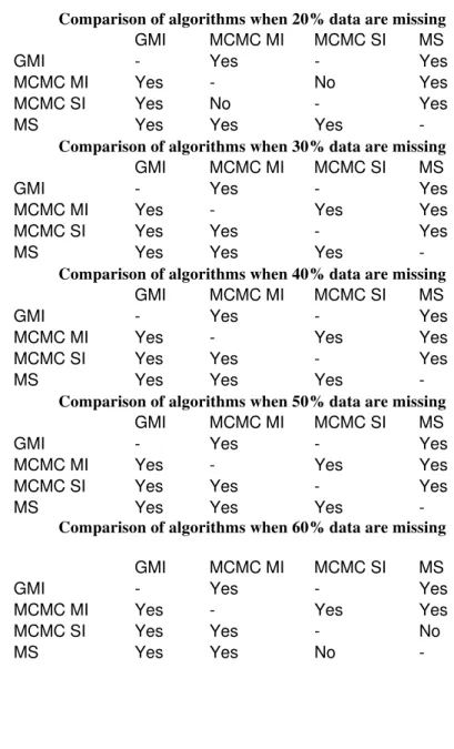
Table A2: Multiple Pairwise Comparisons among the imputation algorithms

Comparison of algorithms when 20% data are missing

GMI - Yes - Yes

MCMC MI Yes - No Yes

MCMC SI Yes No - Yes

MS Yes Yes Yes -

GMI - Yes - Yes

MCMC MI Yes - Yes Yes

MCMC SI Yes Yes - Yes

MS Yes Yes Yes -

GMI - Yes - Yes

MS Yes Yes Yes -

GMI - Yes - Yes

MS Yes Yes Yes -

GMI - Yes - Yes

MCMC SI Yes Yes - No