Modeling of very low frequency (VLF) radio wave signal profile due to solar flares using the GEANT4 Monte Carlo simulation coupled with ionospheric chemistry

(1)

www.atmos-chem-phys.net/13/9159/2013/ doi:10.5194/acp-13-9159-2013

Atmospheric

Chemistry

and Physics

Geoscientiic

Modeling of very low frequency (VLF) radio wave signal profile due

to solar flares using the GEANT4 Monte Carlo simulation coupled

with ionospheric chemistry

S. Palit1, T. Basak2, S. K. Mondal1, S. Pal1, and S. K. Chakrabarti2,1

1_{Indian Centre for Space Physics, 43-Chalantika, Garia Station Road, Kolkata-700084, India} 2_{S N Bose National Centre for Basic Sciences, JD Block, Salt Lake, Kolkata-700098, India}

Correspondence to:S. K. Chakrabarti (chakraba@bose.res.in)

Received: 3 December 2012 – Published in Atmos. Chem. Phys. Discuss.: 7 March 2013 Revised: 25 July 2013 – Accepted: 25 July 2013 – Published: 16 September 2013

Abstract. X-ray photons emitted during solar flares cause ionization in the lower ionosphere (∼60 to 100 km) in ex-cess of what is expected to occur due to a quiet sun. Very low frequency (VLF) radio wave signals reflected from the D-region of the ionosphere are affected by this excess ioniza-tion. In this paper, we reproduce the deviation in VLF signal strength during solar flares by numerical modeling. We use GEANT4 Monte Carlo simulation code to compute the rate of ionization due to a M-class flare and a X-class flare. The output of the simulation is then used in a simplified iono-spheric chemistry model to calculate the time variation of electron density at different altitudes in the D-region of the ionosphere. The resulting electron density variation profile is then self-consistently used in the LWPC code to obtain the time variation of the change in VLF signal. We did the modeling of the VLF signal along the NWC (Australia) to IERC/ICSP (India) propagation path and compared the re-sults with observations. The agreement is found to be very satisfactory.

1 Introduction

The most prominent causes of daytime lower ionospheric modulation (other than the diurnal variation) are the solar flares. The lowest part of the ionosphere, namely, the D-region, formed in the daytime due mainly to the solar UV radiation, is significantly affected by these flares. The X-ray and γ-ray from the solar flares penetrate down to the lower ionosphere causing enhancements of the electron and

the ion densities (Mitra, 1974), though the part of the photon spectrum ranging from∼2 to 12 keV is responsible for the modulation at the reflection heights of very low frequency (VLF) radio waves. The VLF signal (3–30 kHz) reflected mainly from the D-region ionosphere carries information of such enhancements. By analysing these signals between a transmitter and a receiver one could, for example, obtain en-hancements in the electron-ion densities during such events (McRae et al., 2004).

In general, the entire radiation range of EUV, solar Lyman-α, β, X-ray and γ-rays of solar origin (Madronich and Flocke, 1999) and from compact and transient cosmic ob-jects as well as protons from cosmic rays and solar events act as perturbative sources and lead to the evolution of the entire atmospheric chemistry. The amount of energy deposited and the altitudes of deposition depend on the incoming radiation energy. Thus the chemical changes in different layers vary. Many workers have studied these changes theoretically as well as using laboratory experiments. In F2 region, the chem-istry is simpler withN+, H+and O+with O+as the domi-nant ions (Mitra, 1974). Abundance of O+depends on solar UV rays (Wayne, 2000). Similarly O+andN+are dominant in F1 region and their densities are governed by EUV of 10– 100 nm range (Mitra, 1974). E-region is mostly filled up by O2, N2 and NO molecules. During higher energetic X-ray

emission (1–10 nm), O2+ and N2+ are produced. Here, the

(2)

of the D-region is dominated by hard X-ray andγ Ray in-jection from flares and Gamma Ray Bursts (Mitra, 1974; Wayne, 2000; Thomson et al., 2001; H¨oller et al., 2009; Tri-pathi et al., 2011; Mondal et al., 2012). It has nearly similar ion constituents as in the E-region along with hydrated ions like O2+(H2O)n, H+(H2O)n, etc. Several authors such as

Mi-tra (1974), Mcrae (2004), Pal et al. (2012b), studied D-region electron density in detail. Beside these radiation events, reg-ular solar proton events (SPE) having energies 1–500 MeV affect the atmospheric chemistry drastically as one such pro-ton can ionize millions of molecules. Joeckel et al. (2003) reported interesting observations on14CO during SPE. Hol-loway and Wayne (2010), Jackman et al. (2001), Verronen et al. (2005), etc. have reported the effects on the concentrations of14CO, NO, NO2and O3in mesospheric and stratospheric

regions.

Because the earth’s ionosphere (and atmosphere in gen-eral) is a gigantic, noisy, yet free of cost detector of cosmic radiation, study of the evolution of its chemical composi-tion in presence of high energy phenomena (both photons and charged particles) is of utmost importance not only to interpret the results of VLF and other radio waves through it, but also to understand long-term stability of this sensitive system. In the present paper, we apply the GEANT4 simula-tion (applicable to any high energy radiasimula-tion detector) only to understand the changes in the D-region electron density (Ne) during flares as the ion-chemistry leaves negligible

im-pression on VLF propagation characteristics. For that reason knowledge of only the dominant chemical processes in the D-region ionosphere would be enough to study the modula-tion due to events like solar flares (Rowe et al., 1974; Mi-tra, 1981; Chamberlain, 1987). One such simplified model, namely, the Glukhov–Pasko–Inan (GPI) model (Glukhov et al., 1992) can be applied for the events which cause excess ionization in the D-region. Inan et al. (2006) used this model (though modified for lower altitudes) to find the effects of Gamma Ray Bursts on the state of ionization. The model has also been adopted successfully by Haldoupis (Haldoupis et al., 2009) for his work on the early VLF perturbations asso-ciated with transient luminous events.

In the present paper, we model the VLF signal variation due to the D-region ionospheric modulation during solar flares by combining a Monte Carlo simulation (GEANT4) for electron-ion production with the GPI model in the D-region to find the rate of free electron production at differ-ent altitudes by X-rays and γ-rays emitted from flares. Fi-nally, the Long-Wave Propagation Capability (LWPC) code (Ferguson, 1998) has been used to simulate changes in VLF amplitude due to resulting variations of the electron num-ber density. The LWPC code computes the amplitude and phase of the VLF signal for any arbitrary propagation path and ionospheric conditions along the path, including the ef-fects of the earth’s magnetic field. It uses the exponential D-region ionosphere defined by Wait and Spies (1964) and wave guide mode formulations developed by Budden (1951).

This program has been used by many workers and is quiet successful for modeling of long-range propagation of VLF signals even in presence of ionospheric anomalies (Grubor et al., 2008; Rodger et al., 1999; Chakrabarti et al., 2012; Pal et al., 2012a, b). Instead of Wait’s model for the D-region iono-sphere, we used our own result for that part of the ionoiono-sphere, by incorporating the results from the GEANT4 Monte Carlo simulation and the GPI scheme in the LWPC program.

We compared the simulated VLF signal amplitude devia-tions due to the effect of solar flares with those of the ob-servational data detected by the ground based VLF receiver of the Ionospheric and Earthquake Research Centre (IERC) of Indian Centre for Space Physics (ICSP). To illustrate the success of our method, we use one X2.2 type and one M3.5 type solar flare data which occurred on 15 and 24 February 2011, respectively, and compare with the predicted VLF out-put from our model. Our interest is to reproduce the change in the VLF signal during the solar event and examine the de-cay pattern of the signal due to the long recovery time.

The organization of the paper is as follows: in Sect. 2, we present the observational data. In Sect. 3, we present detailed procedures to model the data. This includes successive us-age of the GEANT4 simulation, GPI scheme and the LWPC code. In Sect. 4, we present the results of our modeling which we compared with our observed data. Finally, in Sect. 5 we make concluding remarks.

2 Observational data

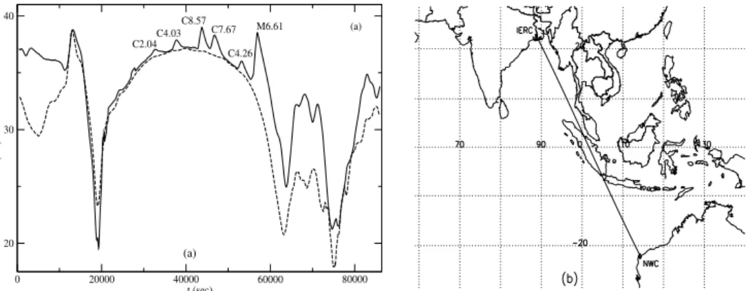
The VLF receivers at the Indian Centre for Space Physics (ICSP) are continuously monitoring several worldwide VLF transmitter signals including NWC (19.8 kHz), VTX (18.2 kHz) and JJI (22.2 kHz). We use the VLF data for the NWC to IERC/ICSP propagation path (distance 5691 km) to compare with our simulation results. In Fig. 1a we present an example of variations of the NWC signal at 19.8 kHz for a typical solar active day (solid curve), with many flares and a normal “quiet” day (dashed curve). There is a sudden rise of wave amplitude followed by a slow decay associated with each of the flares. SoftPAL instrument was used in obtaining the data. In the present paper, we analyze stronger flares (one X2.2 type and one M3.5 type) to begin with. In future, we shall target weaker flares as they require more careful sub-traction of the background. While analysing flares in ques-tion, we use the GOES and RHESSI satellite data (Sui, et al., 2002) to obtain the light curve and spectrum of those flares.

3 The Model

3.1 GEANT4 Monte Carlo simulation

(3)

0 20000 40000 60000 80000 20

30 40

M6.61 C4.26 C7.67 C8.57 C4.03 C2.04

t (sec)

A (dB)

(a)

Fig. 1. (a)The amplitude of VLF signal transmitted from the NWC (19.8 kHz) station, as a function of time (in IST = UT + 5.5 h) as recorded at IERC(ICSP), Sitapur, India, on the 18 February 2011. Six solar flares of different classes (C2.04 at 09:04 UT, C4.03 at 10:21 h, C8.57 at 12:03 h, C7.67 at 12:54 h, C4.26 at 14:41 h and M6.61 at 15:42 h) could be seen. A solar-quiet day data is also presented (dotted line) for comparison which was recorded on 12 February 2011.(b)The propagation path from NWC/Australia to IERC(ICSP)/Sitapur, India.

energy radiations. The earth’s ionosphere is a giant detec-tor and as such, the software used to analyze detecdetec-tors in high energy physics could be used here as well. Most of the ionizations occur in the ionosphere due to the collision of molecules with secondary electrons produced by initial photo-ionization. The program includes sufficiently adequate physical processes for the production of electron ion pairs in the atmosphere by energetic photon interactions.

GEANT4 (GEANT is the abbreviation of Geometry and Tracking) is a openly available and widely tested toolkit (freely available from the website http://geant4.cern.ch/). The Monte Carlo processes in this application deal with the transport and interaction of particles with matter in a pre-defined geometry and store all the information of track, na-ture and number of secondaries efficiently. With this appli-cation we can find accurately the ionization processes and tracks without any prior knowledge and assumption of chem-ical or physchem-ical model of the region. The included electro-magnetic processes related with X-ray incidence are well developed and suitable for application in the context of the ionosphere. For simulation with UV, the application at this stage is not quite suitable, but with some development in the toolkit area, it is possible to use it for Monte Carlo simulation with UV and EUV photons in the ionosphere. We simulated only the rate of ionization at different altitudes due to solar X-ray photons during flares using GEANT4. For the chem-istry part related to the interaction of the produced electron, ions and the neutrals in the D-region ionosphere, we adopt the GPI scheme.

The earth’s atmosphere, constructed in the detector con-struction class consists of concentric spherical shells, so that the atmosphere is divided into several layers. The distribution of layers is as follows, 100 layers above the earth surface, 1 km each followed by 20 layer above this, 5 km each and 12 more layers, 25 km each. They are formed with average molecular densities and other parameters at those heights.

The data is obtained from NASA-MSISE-90 atmospheric model (Hedin, 1991) of the atmosphere.

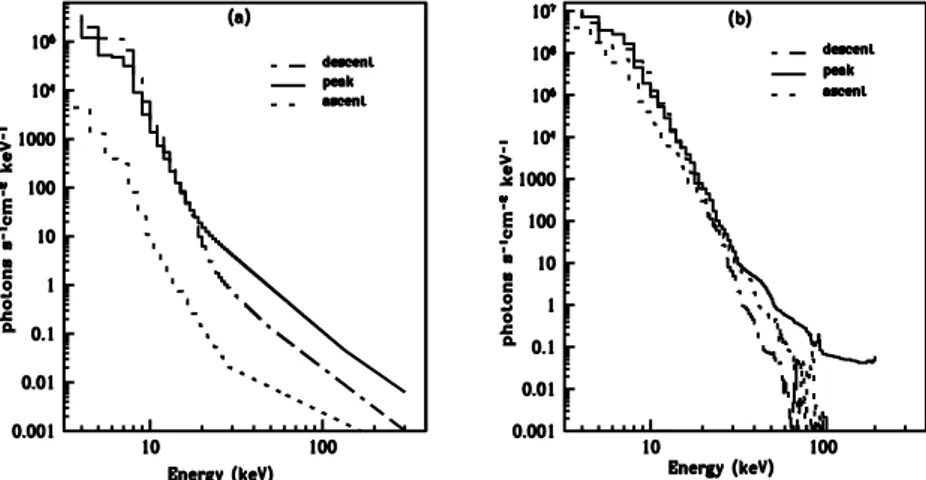
Initially, the Monte Carlo process is triggered by primary particle generation class of GEANT4 with photons of energy ranging from 1–100 keV. We are not interested in higher en-ergy gamma ray photons as their enen-ergy deposition height is much lower than that of the D-region ionosphere. First a uniform spectrum (equal number of photons per keV bin) is chosen for input in primary generation class, such that the incident photons in a specific bin have random ener-gies within the range of the bin. This gives a distribution of electron-ion production rate in a matrix form, theijt h ele-ment of which gives the electron production rate (cm−3s−1) init hkm above sea level due to the incident photons in the jt hkeV bin. We produce such altitude dependent distribu-tion by simuladistribu-tion with different incident angles of the pho-tons. The real altitude distributions of electron-ion produc-tion rate during a flare are obtained by multiplicaproduc-tion of the matrix of corresponding time (hence angle of incidence) with the actual flux spectrum (see Fig. 2) at that time. For this we collect the back-ground subtracted solar spectra during the flares from RHESSI satellite data (http://hesperia.gsfc. nasa.gov/rhessi2/). This method helps us to save a significant amount of computation time.

(4)

Fig. 2.Spectra at three phases (dotted: ascent phase; solid: peak; dash-dotted: descent phase) of the(a)M-class flare and the(b)X-class flare which are used in this paper. The spectra were obtained from the RHESSI satellite data and the OSPEX software.

Fig. 3.Electron production rates per unit volume at peak times for the(a)M-class flare and the(b)X-class flare assuming the sun to be at zenith.

In Fig. 3 we show the altitude distribution of the rate of electron density produced by the spectra shown in Fig. 2a and b at the peak flare time assuming the sun to be at the zenith.

From Fig. 3a and b, it is evident that the ionization effect due to the solar X-rays is dominant in the D-region (∼60– 100 km) only. The simulation also shows that the altitude of maximum ionization is somewhat lower for X-class flare (∼81 km) than that of (∼88 km) M-class. This is consistent with the fact that the relative abundance of high energy pho-tons is larger in X-class spectra.

The effects of the zenithal variation of the sun is included in the simulation to account for the variation of the flux in long duration flares. Fig. 4 shows the simulated electron pro-duction rate (cm−3_s−1_{) at various altitudes for the M-class}

spectrum (Fig. 2a) at the flare peak if it had occurred at dif-ferent times of the day. In finding the rate of production of electron density over the whole period of the flares, we con-volve the normalized (by corresponding spectrum) electron

density distribution profiles with the light curves of the flares, taking into account the dependency of the electron density on the angular positions.

We simulate the condition at the middle of the VLF prop-agation path (Fig. 1b) and assume that the resulting electron density distribution apply for the whole path. Along the prop-agation path in question, the solar zenith angle variation is at the most∼30◦. Figure 4 shows that the approximation is jus-tifiable, especially if the solar zenithal angle is close to 0 at the mid-propagation path.

(5)

Fig. 4.Variation of electron production rates with the angular posi-tion of the sun at different heights assuming an M-class spectrum.

3.2 The GPI model

Our next goal is to compute the changes in atmospheric chemistry due to the flare. These could be obtained using a simplified model, such as the GPI model (Glukhov et al., 1992). In this model, the number density evolution of four types of ion species are taken into account for the estimation of the ion density changes in the D-region. These are: elec-trons, positive ions, negative ions and positive cluster ions. The positive ions N+comprise of mainly O+₂ and NO+₂. The negative ions N− include O−₂, CO−₃, NO−₂, NO−₃ etc. The positive cluster ionsN_x+are usually of the form H+(H2O)n.

The GPI model is meant for the nighttime lower ionosphere. Modified set of equations exists (Lehtinen and Inan, 2007), which are applicable at even lower heights (∼50 km), where the inclusion of negative ion clustersN_x−is important and the scheme has been used for the daytime lower ionosphere also (Inan et al., 2007). However, for the altitudes (above 60 km) of our interest, where the VLF wave is reflected, the simpli-fied GPI model is sufficient. While considering the solar pho-tons, we concentrate only on the ionization produced by the X-rays from solar flares, not from the regular UV and Lyman alpha lines etc. Though it is a simplification, this will produce good results as long as the electron-ion production rates due to X-ray dominates over the regular production rates. The model is suitable for the strong flares (at least higher C-class and above) and is valid up to the time of recovery when the above approximation holds.

According to the model, the time evolution of the ion den-sities follow ordinary differential equations, the right hand sides of which are the production (+ve) and loss (-ve) terms.

dNe

dt =I+γ N

−₋_βN

e−αdNeN+−αdcNeNx+, (1)

dN−

dt =βNe−γ N

−

−αiN−(N++Nx+), (2)

dN+

dt =I−BN

+

−αdNeN+−αiN−N+, (3)

dN+

x

dt =BN

+₋_αc

dNeNx+−αiN−Nx+. (4)

The neutrality of the plasma requires,

N−+Ne=N++Nx+. (5)

Here,β is the electron attachment rate (Rowe et al., 1974), the value of which is given by,

β=10−31NO2NN2+1.4×10

29₍300

T )e

(−600

T )_N2

O2. (6)

NO2 andNN2 represent the number densities of molecular

Oxygen and Nitrogen respectively, andT is the electron tem-perature. The neutral atom concentrations at different alti-tudes, required for the calculations of the coefficients, were obtained from the NASA-MSISE atmospheric model. The detachment coefficient, i.e., the coefficient of detachment of electrons from negative ions has contributions from both photodetachment (at daytime) and also processes other than photodetachment. The coefficient for the photodetachment process is∼10−2to 5×10−1and for the other process it is ∼10−1to 10−2at 80 km (Bragin, 1973). According to Lehti-nen and Inan (2007) and Pasko and Inan (1994), the value of the detachment coefficientγ varies widely from 10−23_N_s−1

to 10−16_N_s−1_{. Following Glukhov et al. (1992) the value of}

γis taken to be 3×10−18_N_s−1_{, where}_N_{is the total number}

density of neutrals. In our calculations the value ofγ comes out to be 2.4×10−2_{at 75 km to 6.6}_×₁₀−3_{at 84 km, which}

is reasonable.

Previous studies (Lehtinen and Inan, 2007; Rowe et al., 1974) predict that the effective coefficient of dissocia-tive recombination αd may have values from 10−7 to 3×

10−7cm−3s−1. We have used 3×10−7cm−3s−1forαd.

The effective recombination coefficient of electrons with positive cluster ions α_dc has the value ∼10−6– 10−5cm−3s−1. Here the value of 10−5cm−3s−1is adopted as suggested by Glukhov et al. (1992). The value of the ef-fective coefficient of ion–ion recombination processes for all types of positive ions with negative ions is taken to be 10−7_cm−3_s−1_{(Mitra, 1968; Rowe et al., 1974).}_B_{is the}

ef-fective rate of conversion from the positive ion (N+_{) to the}

positive cluster ions (N_x+) and has the value 10−30N2s−1 (Rowe et al., 1974; Mitra, 1968), in agreement with Glukhov et al. (1992).

The termI, which corresponds to the electron-ion produc-tion rate, can be written asI=I0+Ix. HereI0is from the

(6)

30000 36000 10-6

10-5

10000 20000 30000

10-6 10-5 10-4

30000 36000

10-1 100 101 102

10000 20000 30000

100 101 102 103

(a)

(b)

(c)

_(d)

Elec. prod. (cm s )

X-ray flux (Watt m )

-3 -1

-2

t (s) [started from 06:56:40 UT] t (s) [started from 01:23:20]

80 km 76 km

72 km 68 km 80 km

72 km 68 km

76 km

64 km _{64 km}

Fig. 5.Light curves of the flares from GOES satellite of an(a)M-class and(b)X-class flare. The time variation of the electron production rates at different heights as obtained from GEANT4 simulation for these flare respectively are shown in(c)and(d).

Fig. 6.Electron density at different layers during the(a)M-class and(b)X-class flares.

ambient distributions of ions. In our case, I0 corresponds

grossly to the part produced by the background ultraviolet ray, Lyman alpha lines, etc. from the sun, producing the D region. The termIxis the modulated component of the

ion-ization rate. HereIxis generated by the X-ray photons (in the

energy range from 2 to 12 keV, important for the D-region) coming from the solar coronal region during solar flares only. To account for the time variation of the number density of the ion species, we divide each term into a constant and a time dependent parts, i.e.,Ne is replaced withN0e+Ne(t ),

N+withN₀++N+(t ),N−withN₀−+N−(t )andN_x+with N_0x++N+

x(t ). A set of equations governing the equilibrium

conditions can be obtained from Eqs. (1–4), by replacing

the ion density terms with their ambient values,I byI0and

equating the rates to zero (Glukhov et al., 1992).

Using the conditions of equilibrium and the above replace-ments in Eqs. (1–4), we get the following set of equations

dNe

dt =Ix+γ N

−

−βNe−αd(N0eN++NeN₀++NeN+)

−αc_d(N0eNx++NeN₀+_x+NeNx+), (7)

dN−

dt =βNe−γ N

− −

αi[N₀−(N++Nx+)+N

−_(N+

0 +N

+

(7)

100 1000 65

70 75 80

h (km)

electron density N (cm )e -3

(a)

100 1000 10000 65

70 75 80

electron density N (cm )

h (km)

e -3

(b)

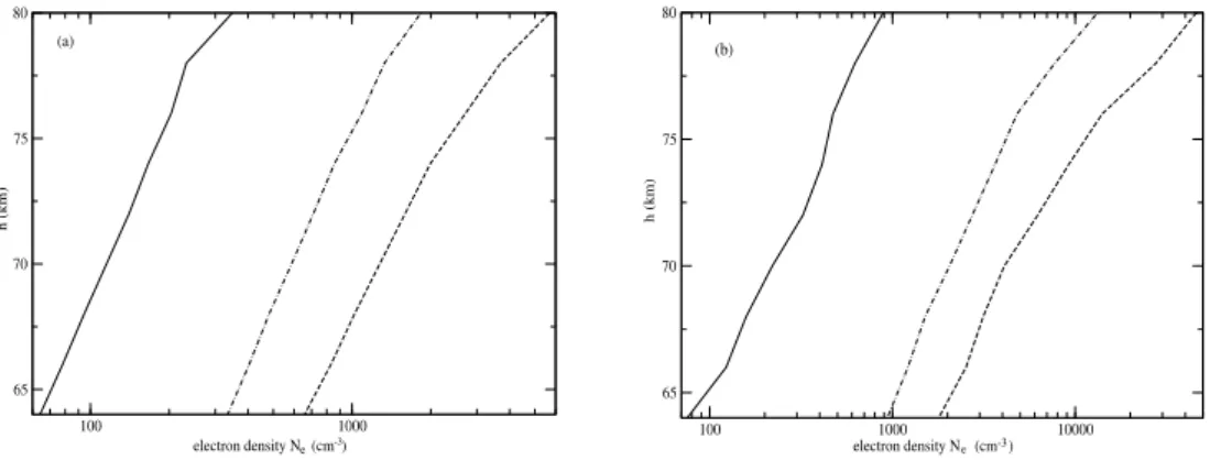
Fig. 7.Altitude profiles of electron density as obtained from GPI model at three different times for an(a)M-class and(b)X-class flare. Solid line shows the ambient profile before the beginning of the flare while the dashed and the dot-dashed lines represent the profile during the peak and at a time during recovery.

dN+

dt =Ix−BN

+

−αd(N0eN++NeN₀++NeN+)

−αi(N₀−N++N−N₀++N−N+), (9)

dN_x+ dt =BN

+₋_αc

d(N0eNx++NeN_0x++NeNx+)

−αi(N0−N

+

x +N−N

+

0x+N

−_N+

x). (10)

The ambient values of the electron and ion densities are ob-tained from the IRI model (Rawer et al., 1978). Unperturbed negative ion density N₀− is obtained from the relationship N₀−=λN0e, whereλis the relative composition of the

neg-ative ions. The values of positive ion densities are calculated from the charge neutrality condition, i.e.,

N0e+N0−=N

+

0x+N

+

0. (11)

Using the ionization rate per unit volume (Ix) obtained from

the GEANT4 simulation and the coefficients of the ODEs calculated from MSIS data, we solve the ODEs (Eqs. 7–10) by Runge–Kutta method to find the residual electron density at various altitudes during the course of the flare.

Figure 6a and b show the electron density variations at different altitudes throughout the flares. The enhancement in electron density from ambient values can be clearly seen.

Figure 7a and b shows the altitude variations of the elec-tron densities as obtained from the GPI model. These are plotted at three different times including the peak time. The times are shown by arrows in Fig. 6a and b, The ambient electron density during the X-class flare was higher than that of the M-class flare. This is because the background X-ray flux during the X-class flare was stronger.

Though we do not expect drastic changes in the VLF ra-dio signal due to the changes in the chemical composition at the altitudes of our interests, for the sake of completeness, we show in Fig. 8, the altitude profile of three types of ion densities at three different times evaluated numerically from the GPI scheme. We show this for the X-class flares only. It

is to be noted that they are the outcome of simplified chemi-cal model devoid of physichemi-cal processes such as the transport of ions through the layers of Ionosphere etc. These processes are being studied and would be reported elsewhere.

3.3 Modeling VLF response with LWPC

Now that we have the electron densities (Ne) at various

al-titudes, we can use them to obtain the time variation of the deviation of the VLF signal amplitude during a flare event. We use the Long-Wave Propagation Capability (LWPC) code (Ferguson, 1998) to accomplish this. LWPC is a very versa-tile and well-known code and the current LWPC version has the scope to include arbitrary ionospheric variations as the input parameters for the upper waveguide. The electron den-sity profiles (Fig. 6) represent the modulated D-region iono-sphere due to the solar flares and can be used as the inputs of the LWPC code to simulate the VLF signal behavior. The electron-neutral collision frequency in the lower ionosphere plays an important role for the propagation of VLF signals. We used the collision frequency profiles between electrons and neutrals as described by Kelley (2009). This is given by the following equation,νe(h)=5.4×10−10nnT1/2, where

nn andT are the neutral density (in cc) and electron

tem-perature (in K), respectively. Assuming the temtem-perature of the electrons and the ions are same and using the ideal gas equation, the above equation can be expressed as (Schmitter, 2011),νe(h)=3.95×1012T−1/2exp(−0.145h).

4 Results

(8)

1000 10000

Negative ion density N (cm )

65 70 75 80

h (km)

- -3

(a)

1 100 10000

Positive ion density N (cm )

65 70 75 80

h (km)

+ -3

(b)

1000 10000

Positive cluster ion density N (cm )

65 70 75 80

h (km)

+ -3

x (c)

Fig. 8.Altitude profiles of three types of ion densities as obtained from the GPI scheme:(a)negative ions,(b)positive ions, and(c)positive cluster ions. The solid, dashed and dot-dashed lines represent respectively the ambient profile, the profile at the peak and the profile at a time during recovery of the X-type flares as discussed in the text.

Fig. 9.Simulation results of VLF amplitude modulations (dotted line) and corresponding observed VLF data (solid line) are plotted with UT for an(a)M-class flare and an(b)X-class flare, respectively.

also the subtraction is made, but with a flat VLF profile ob-tained from the ambient electron density shown in Fig. 6a and b. The variation of ambient ion densities during the course of the day affects the recombination process of the modulated D-region ionosphere when the flare duration is long. This is evident from Eqs. (7)–(10) that the rate of change of the elec-tron density depends on the ambient concentration. If it was not the case, the subtraction would have made no difference.

(9)

the modelled slope becomes gradually higher than that of the observation. The M-class flare occurred at the local afternoon when the diurnal ambient electron densities at various alti-tudes are decreasing. During the decay of the flare when the effect of ambient ion densities start to dominate, observed slope of decay become higher in value (than that predicted from the model, where this effect is ignored) while still fol-lowing the trend of variation of observed VLF amplitude at that time. The X-class flare, on the other hand, occurred in the morning when ambient electron densities are increasing with time due to the diurnal variation. In this case, the slope of observed decay is a lower.

It can also be seen (comparing Fig. 9 with Fig. 6) that the differences in slopes of decay between the models and the observations start to occur when the electron densities fall be-low a certain level for both the flares (∼2000 cm−3_{at 80 km).}

Furthermore, since the M-class flare spectrum is relatively softer than that of the X-class one, the ambient electron den-sity starts to dominate the VLF amplitude a bit earlier during decay of the M-class flare. We can see that the deviation of the modelled slope from the observed one starts earlier for M-class flare than the other.

5 Concluding remarks

In this paper, we have used a three step approach to com-pute the deviation of the VLF signal amplitude during a so-lar fso-lare. The steps are (i) GEANT4 Monte Carlo simulation for ionization rate estimation, (ii) GPI-scheme of ionospheric chemistry analysis and finally (iii) LWPC modeling of sub-ionospheric VLF signal propagation. This combined model is self-consistent, realistic and uses a few justifiable assump-tions. Our method is capable of estimating the VLF signal behavior directly using the corresponding incident solar flux variation on D-region ionosphere during a solar flare.

In our model computation, we have ignored the effects of the variation of ambient concentrations, i.e., the diurnal variations (ambient) ofN0e,N0+, etc. are not taken into

ac-count during the flares while solving the ODEs. So as long as the electron densities produced by the X-rays from the flares dominate over the ambient electron densities due to regular ionization sources, such as the ultraviolet, Lyman alpha pho-tons, etc., the model should follow observed variations in the VLF data. We can see in Fig. 9 that it is in fact the case. In future, we shall study the effects of the occurrence times of the flare on the modeling and also the effects of radiation on chemical changes in other altitudes using our method.

We are interested in further modeling of the ionization ef-fect of EUV and UV photons so that we can remove the discrepancies between the modelled and observed decay of the perturbation and extend the modeling throughout the du-ration of the flare. This will require a knowledge of some more details of the ionospheric chemistry and fluid dynam-ics. Also, the inclusion of inhomogeneous distribution of

ionospheric dynamics during flares and adoption of more re-alistic values of ionospheric parameters will lead to results in better agreement with observations. In future, these modifi-cations will be made in the time analysis of the flare decay and the sluggishness of ionosphere.

Acknowledgements. Sourav Palit and Sujay Pal acknowledge

MOES for financial support. Sushanta K. Mondal and Tamal Basak acknowledge CSIR fellowship.

Edited by: F.-J. L¨ubken

References

Agostinelli, S., Allison, J., Amako, K., Apostolakis, J., Araujo, H., Arce, P., Asai, M., Axen, D., Banerjee, S., Barrand, G., Behner, F., Bellagamba, L., Boudreau, J., Broglia, L., Brunengo, A., Burkhardt, H., Chauvie, S., Chuma, J., Chytracek, R., Coop-erman, G., Cosmo, G., Degtyarenko, P., Dell Acqua, A., De-paola, G., Dietrich, D., Enami, R., Feliciello, A., Ferguson, C., Fesefeldt, H., Folger, G., Foppiano, F., Forti, A., Garelli, S., Giani, S., Giannitrapani, R., Gibin, D., Gomez Cadenas, J. J., Gonzalez, I., Gracia Abril, G., Greeniaus, G., Greiner, W., Grichine, V., Grossheim, A., Guatelli, S., Gumplinger, P., Hamatsu, R., Hashimoto, K., Hasui, H., Heikkinen, A., Howard, A., Ivanchenko, V., Johnson, A., Jones, F. W., Kallenbach, J., Kanaya, N., Kawabata, M., Kawabata, Y., Kawaguti, M., Kelner, S., Kent, P., Kimura, A., Kodama, T., Kokoulin, R., Kossov, M., Kurashige, H., Lamanna, E., Lamp, T., Lara, V., Lefebure, V., Lei, F., Liendl, M., Lockman, W., Longo, F., Magni, S., Maire, M., Medernach, E., Minamimoto, K., MoradeFreitas, P., Morita, Y., Murakami, K., Nagamatu, M., Nartallo, R., Nieminen, P., Nishimura, T., Ohtsubo, K., Okamura, M., O’Neale, S., Oohata, Y., Paech, K., Perl, J., Pfeiffer, A., Pia, M. G., Ranjard, F., Rybin, A., Sadilov, S., DiSalvo, E., Santin, G., Sasaki, T., Savvas, N., Sawada, Y., Scherer, S., Sei, S., Sirotenko, V., Smith, D., Starkov, N., Stoecker, H., Sulkimo, J., Takahata, M., Tanaka, S., Tcherni-aev, E., SafaiTehrani, E., Tropeano, M., Truscott, P., Uno, H., Urban, L., Urban, P., Verderi, M., Walkden, A., Wander, W., We-ber, H., Wellisch, J. P., Wenaus, T., Williams, D. C., Wright, D., Yamada, T., Yoshida, H., Zschiesche, D.: GEANT4 simulation toolkit, Nucl. Instrum. Meth. A, 506, 250–303, 2003.

Budden, K. G.: The reflection of very low frequency radio waves at the surface of a sharply bounded ionosphere with superimposed magnetic field., Phil. Mag., 42, 833–843, 1951.

Bragin, A. Y.: Nature of the lower D region of the Ionosphere., Na-ture, 245, 450–451, doi:10.1038/245450a0, 1973.

Chakrabarti, S. K., Pal, S., Sasmal, S., Mondal, S. K., Ray, S., Basak, T., Maji, S. K., Khadka, B., Bhowmik, D., and Chowd-hury, A. K.: VLF campaign during the total eclipse of July 22nd, 2009: Observational results and interpretations, J. Atmos. Sol.-Terr. Phys., 86, 65–70, 2012.

Chamberlain, J. W. and Hunten, D. M.: Theory of planetary atmo-spheres : an introduction to their physics and chemistry, Aca-demic, San Diego, CA, USA, 1987.

(10)

docu-ment 3030, Space and Naval Warfare Systems Center, San Diego, CA, USA, 1998.

Glukhov V. S., Pasko V. P., and Inan U. S.: Relaxation of transient lower ionospheric disturbances caused by lightning-whistler-induced electron precipitation bursts, J. Geophys. Res., 97, 16971–16979, 1992.

Grubor, D. P., ˇSuli´c, D. M., and ˇZigman, V.: Classification of X-ray solar flares regarding their effects on the lower iono-sphere electron density profile, Ann. Geophys., 26, 1731–1740, doi:10.5194/angeo-26-1731-2008, 2008.

Hedin, A. E.: Extension of the MSIS Thermosphere Model into the middle and lower atmosphere, Geophys. Res. Lett., 96, 1159– 1172, 1991.

Haldoupis, C., Mika, A., and Shalimov, S.; Modeling the relaxation of early VLF perturbations associated with transient luminous events, J. Geophys. Res., 114, A00E04, 11 pp., 2009.

H¨oller, H., Betz, H.-D., Schmidt, K., Calheiros, R. V., May, P., Houngninou, E., and Scialom, G.: Lightning characteristics ob-served by a VLF/LF lightning detection network (LINET) in Brazil, Australia, Africa and Germany, Atmos. Chem. Phys., 9, 7795–7824, doi:10.5194/acp-9-7795-2009, 2009.

Holloway, A. M. and Wayne, R. P.: Atmospheric Chemistry (book), RSC Publishing, 2010.

Inan, U. S., Cohen, M. B., Said, R. K., Smith, D. M., and Lopez, L. I.: Terrestrial gamma ray flashes and lightning discharges, Geo-phys. Res. Lett., 33, L18802, 5 pp., doi:10.1029/2006GL027085, 2006.

Inan, U. S., Lehtinen N. G., Moore R. C., Hurley K., Boggs S., Smith D. M., Fishman G. J.; Massive disturbance of the daytime lower ionosphere by the giant g-ray flare from magnetar SGR 1806-20 ; Geophys. Res. Lett., 34, L08103, doi:10.1029/2006GL029145, 2007.

Jackman, C. H., McPeters, R. D., Labow, G. J., Fleming, E. L., Praderas, C. J., and Russel, J. M.: Northern Hemisphere atmo-spheric effects due to the July 2000 solar proton event, Geophys. Res. Lett., 28, 2883–2886, doi:10.1029/2001GL013221, 2001. Joeckel, P., Brenninkmeijer, C. A. M., Lawrence, M. G., and

Sieg-mund, P.: The detection od solar proton produced14CO, Atmos. Chem. Phys., 3, 999–1005, doi:10.5194/acp-3-999-2003, 2003. Kelley, M. C.: The Earths Ionosphere, Plasma Physics and

Electro-dynamics, chapter 2.2, Academic Press, second edition, 2009. Lehtinen N. G. and Inan U. S.: Possible persistent ionization

caused by giant blue jets, Geophys. Res. Lett., 34, L08804, doi:10.1029/2006GL029051, 2007.

Madronich, S. and Flocke, S.: The role of solar radiation in at-mospheric chemistry, Environmental Photo-chemistry (book), Springer, 1999.

Mariska, J. T. and Oran, E. S.: The E and F region ionospheric re-sponse to solar flares: 1. Effects of approximations of solar flare EUV fluxes, J. Geophys. Res., 86, 5868–5872, 1981.

McRae, W. M. and Thomson, N. R.: Solar flare induced ionospheric d-region enhancements from VLF phase and amplitude observa-tions, J. Atmos. Sol. Terr. Phys., 66, 77–87, 2004.

Mitra, A. P.: A review of D-region processes in non-polar latitudes, J. Atmos. Sol. Terr. Phys., 30, 1065–1114, 1968.

Mitra, A. P.: Ionospheric effects of solar flares, Dordrecht, the Netherlands, D. Reidel Publishing Co., Astrophysics and Space Science Library, 46, 307 pp., 1974.

Mitra, A. P.: Chemistry of middle atmospheric ionization-a review, J. Atmos. Sol. Terr. Phys., 43, 737–752, ISSN 0021-9169, 1981. Mondal, S. K., Chakrabarti, S. K., and Sasmal, S.: Detection of Ionospheric Perturbation due to a Soft Gamma Ray Repeater SGR J1550-5418 by Very Low Frequency Radio Waves, Astro-physics and Space Science, 341, 259–264, 2012.

Pal, S., Chakrabarti, S. K., and Mondal, S. K.: Modeling of sub-ionospheric VLF signal perturbations associated with total solar eclipse, 2009 in Indian subcontinent, Adv. Space Res., 50, 196– 204, 2012a.

Pal, S., Maji, S. K., and Chakrabarti, S. K.: First Ever VLF Monitor-ing of Lunar occultation of a Solar Flare durMonitor-ing the 2010 Annu-lar SoAnnu-lar Eclipse and its effects on the D-region Electron Density Profile, Planet. Space Sci., 73, 310–317, 2012b.

Pasko, V. P. and Inan, U. S.: Recovery signatures of lightning-associated VLF perturbations as a measure of the lower iono-sphere, J. Geophys. Res., 99, 17523–17537, 1994.

Rawer, K., Bilitza, D., and Ramakrishnan, S.: Goals and status of the International Reference Ionosphere, Rev. Geophys., 16, 177– 181, 1978.

Rodger, C. J., Clilverd, M. A., and Thomson, N. R.: Modeling of subionospheric VLF signal perturbations associated with earth-quakes, Radio Sci., 34, 1177–1185, 1999.

Rowe, J. N., Mitra, A. P., Ferraro, A. J., and Lee, H. S.: An ex-perimental and theoretical study of the D-region – II. A semi-empirical model for mid-latitude D-region, J. Atmos. Terr. Phys., 36, 755–785, 1974.

Schmitter, E. D.: Remote sensing planetary waves in the midlatitude mesosphere using low frequency transmitter signals, Ann. Geo-phys., 29, 1287-1293, doi:10.5194/angeo-29-1287-2011, 2011. Sui, L., Holman, G, D., Dennis, B, R., Krucker, S., Schwartz, R, A.,

and Tolbert, K.: Modeling Images and Spectra of a Solar Flare Observed by RHESSI on 20 February 2002, Kluwer Academic Publishers, 245–259, 2002.

Thomson, N. R. and Clilverd, M. A.: Solar flare induced iono-spheric D-region enhancements from VLF amplitude observa-tions, J. Atmos. Sol. Terr. Phys., 63, 1729–1737, 2001.

Tripathi, S. C., Khan, P. A., Ahmed, A., Bhawre, P., Purohit, P. K., and Gwal, A. K.: Proceeding of the 2011 IEEE International Conference on Space Science and Communication (IconSpace) 12–13 July 2011, Penang, Malaysia, 2011.

Verronen, P. T., Seppaelae, A., Clilverd, M. A., Rodger, C. J., Kyroelae, E., Enell, C. F., Ulich, T., and Turunen, E.: Diur-nal variation of ozone depletion during the October-November 2003 solar proton events, J. Geophys. Res., 110, A09S32, doi:10.1029/2004JA010932, 2005.