www.biogeosciences.net/11/7107/2014/ doi:10.5194/bg-11-7107-2014
© Author(s) 2014. CC Attribution 3.0 License.
Multi-factor controls on terrestrial carbon dynamics in
urbanized areas
C. Zhang1,2, H. Tian3, S. Pan3, G. Lockaby3, and A. Chappelka3
1State Key Laboratory of Desert and Oasis Ecology, Xinjiang Institute of Ecology and Geography,
Chinese Academy of Sciences, China
2School of Resources Environment Science and Engineering, Hubei University of Science and Technology, Hubei, China 3International Center for Climate and Global Change Research, School of Forestry and Wildlife Sciences,
Auburn University, Auburn AL, 36849, USA
Correspondence to: H. Tian ([email protected]) and C. Zhang ([email protected])
Received: 14 September 2013 – Published in Biogeosciences Discuss.: 11 November 2013 Revised: 28 October 2014 – Accepted: 3 November 2014 – Published: 16 December 2014
Abstract. As urban land expands rapidly across the globe, much concern has been raised that urbanization may alter the terrestrial carbon cycle. Urbanization involves complex changes in land structure and multiple environmental factors. Little is known about the relative contribution of these indi-vidual factors and their interactions to the terrestrial carbon dynamics, however, which is essential for assessing the effec-tiveness of carbon sequestration policies focusing on urban development. This study developed a comprehensive anal-ysis framework for quantifying relative contribution of indi-vidual factors (and their interactions) to terrestrial carbon dy-namics in urbanized areas. We identified 15 factors belong-ing to five categories, and we applied a newly developed fac-torial analysis scheme to the southern United States (SUS), a rapidly urbanizing region. In all, 24 numeric experiments were designed to systematically isolate and quantify the rel-ative contribution of individual factors. We found that the im-pact of land conversion was far larger than other factors. Ur-ban managements and the overall interactive effects among major factors, however, created a carbon sink that compen-sated for 42 % of the carbon loss in land conversion. Our find-ings provide valuable information for regional carbon man-agement in the SUS: (1) it is preferable to preserve pre-urban carbon pools than to rely on the carbon sinks in urban ecosys-tems to compensate for the carbon loss in land conversion. (2) In forested areas, it is recommendable to improve land-scape design (e.g., by arranging green spaces close to the city center) to maximize the urbanization-induced environmental change effect on carbon sequestration. Urbanization-induced
environmental change will be less effective in shrubland re-gions. (3) Urban carbon sequestration can be significantly improved through changes in management practices, such as increased irrigation and fertilizer and targeted use of vehicles and machinery with least-associated carbon emissions.
1 Introduction
Kuang, 2012a). The urban ecosystems could account for a significant portion of terrestrial carbon (C) storage (Nowak and Crane, 2002; Pataki et al., 2006; Pouyat et al., 2006; Churkina et al., 2010; Davies et al., 2011; Hutyra et al., 2011; Edmondson et al., 2012). Zhang et al. (2012) estimated that urban and developed land accounts for about 6.7–7.6 % of total ecosystem C storage within the southern United States (SUS), which is larger than the pool size of shrubland. The potential for C sequestration in urban vegetation (McPher-son et al., 1997) and soil (Pouyat et al., 2008) has drawn at-tention from both ecologists and decision makers (Poudyal et al., 2010). Municipal interest in climate change mitiga-tion through C offset trading has increased as many cities have established substantial programs, such as tree planting, to increase ecological services of urban ecosystems (Nowak, 2006; Tratalos et al., 2007; Young, 2010). A management strategy for urban and peri-urban land, as suggested by the Intergovernmental Panel on Climate Change (IPCC, 2000), including tree planting, improved waste management, and wood production, could lead to a C sink of 0.3 t C ha−1a−1.
Escobedo et al. (2010) indicated that urban forest manage-ment can create moderate carbon sink in the southeastern United States.
However, the ecological consequence of urbanization is highly complex (Pickett et al., 2011), not only because of the strong spatial heterogeneity of urban ecosystems (Kuang, 2012b), which is composed by land cover types with distinct biogeochemical characteristics (Cannell et al., 1999; Alberti, 2005; Buyantuyev et al., 2010), but also because urbaniza-tion usually results in significant changes in many interact-ing environmental factors that affect ecosystem C processes, such as land conversion from rural to urban land use (Schal-dach and Alcamo, 2007), shifts in disturbance and manage-ment regimes (Kissling et al., 2009; Fissore et al., 2012), and urban-induced climate and atmospheric changes (Ko-erner and Klopatek, 2002; Fenn et al., 2003; Kuttler, 2011; Li et al., 2011). Furthermore, the legacy effect of pre-urban land use changes (Ramalho and Hobbs, 2012) and influences from global climate changes (McCarthy et al., 2010) could also modify the ecosystem’s responses to the urbanization-induced environmental changes. Analyzing the impacts of these changes and their interactive effects will help in our understanding of how regional C cycles are affected by ur-banization, quantifying the impacts of various environmen-tal stresses, and identifying the major factors that control C dynamics of developed areas. Such knowledge can be valu-able for policy makers and managers to predict the long-term ecological consequences of urbanization, to elucidate where management efforts should focus, and to formulate meaning-ful guidelines and tailor strategies for urban C managements. Despite its importance and complexity, urbanization is an often-missing component in global change studies (Kaye et al., 2005; Pouyat et al., 2006). There are several remote sens-ing analyses that addressed the urbanization effect on net pri-mary productivity (NPP) (Imhoff et al., 2000; Milesi et al.,
2003; Lu et al., 2010). With an empirical inventory approach, Cannell et al. (1999) roughly estimated the effects of urban-ization on the C budget of the United Kingdom. Only a few modeling studies have analyzed the responses of regional C dynamics to the environmental changes induced by urban-ization. Many studies suggested that urban land conversion could have a strong negative impact on regional to global C storage (Schaldach and Alcamo, 2007; Svirejeva-Hopkins and Schellnhuber, 2008; Zhang et al., 2008; Eigenbrod et al., 2011). Trusilova and Churkina (2008) compared the im-pacts of different urban-induced environmental changes on the C cycle in Europe and found strong C sequestration due to urbanization-induced atmospheric changes. Milesi et al. (2005) assessed effects of different management prac-tices on the C storage of Unites States urban lawn. Zhang et al. (2012) found that pre-urbanization vegetation type and time since land conversion were closely related to the ex-tent of urbanization effects on C dynamics of the southern Unites States over the last 6 decades. Despite these efforts, a comprehensive study that investigates the dominant envi-ronmental changes and addresses their relative importance on regional C dynamics is still not available, although it has been repeatedly suggested that, due to the complex interac-tions among multiple involving factors, the ecological conse-quences of urbanization could not be fully understood with-out a full set of controlling drivers and their interactions be-ing addressed (Hutyra et al., 2011; Pickett et al., 2011; Ra-malho and Hobbs, 2012).
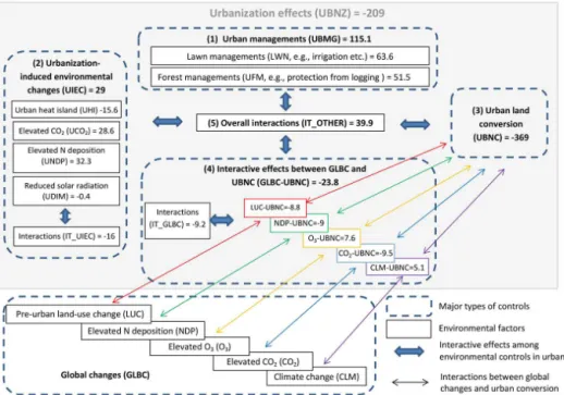
Figure 1.The urbanization (UBNZ) effects on regional carbon dynamics are controlled by four major types of environmental changes, including (1) urban land conversion (UBNC) during which rural land use type is converted to urban and developed land use composed by impervious surfaces, managed urban lawn, and other urban vegetation (e.g., urban forest); (2) urban management (UBMG), including lawn (LWN) management, such as irrigation and fertilization, and urban forest management, such as protection from logging and fire disturbances; (3) urbanization-induced environmental changes (UIECs), including effects of urban heat island (UHI), elevated CO2(UCO2)
and N deposition (UNDP), reduced solar radiation due to air pollution (UDIM), and interactions among these UIEC factors (IT_UIEC); (4) the interactive effects between UBNC and multiple global environmental changes (GLBC–UBNC), including changes in climate (CLM–
UBNC), CO2(CO2–UBNC), N deposition (NDP-UBNC), ozone exposure (O3–UBNC), pre-urban land use change history (LUC–UBNC),
such as cropland conversion and abandonment, and the interactions among all GLBC–UBNC factors. IT_OTHER represents the overall interactive effects among the four major controls (i.e., UBNC, UBMG, UIEC, and GLBC–UBNC). The numbers in the figure show the carbon flux in response to each factor from 1945 to 2007 in the southern United States. Unit: TgC.
study) by identifying the dominant controls on the C dynam-ics and elucidating where management efforts should focus.
2 Factors controlling urbanization effects
To study the effects of urbanization on regional C balance, Zhang et al. (2012) compared the model simulation results of the urbanization scenario (or the “business as usual” sce-nario) against the results from a non-urbanization scenario in which the urbanization process was controlled and all lands remained in pre-urban land types. They found that the ur-banization from 1945 to 2007 resulted in a regional C loss of 0.21 Pg C in the SUS. The study, like others (McCarthy et al., 2010), also indicated that urbanization is not a simple C re-lease process, but involves complex changes in land structure and multiple environment factors, whose effects should not be treated independently. Whenever an ecosystem compo-nent is modified by one environmental stress, the ecosystem’s responses to other factors could also be altered due to the non-linear interactions among the coupled ecosystem com-ponents and processes (Wu, 1999). For example, elevated
CO2in urban areas could be particularly important in
reliev-ing water stress induced by urban heat island effect (Groff-man et al., 2006). Therefore, it is important to consider all the major environmental factors and their interactive effects on C processes when studying the urbanization effects on regional C balance.
In Fig. 1, we generalize the factors that may control the urbanization (UBNZ) effects (descriptions for the abbrevia-tions are found in Fig. 1): (1) urban vegetation is intensively managed. Irrigation, fertilization, and weed disease controls improve lawn productivity (Milesi et al., 2005). Remnant ecosystems in urban areas are generally protected from in-tensive disturbances, such as agricultural soil tillage, wild fire, and commercial logging (Raciti et al., 2011). All of these urban managements (UBMGs) could result in high C density in urban ecosystems, as observed in former stud-ies (Nowak and Crane, 2002; Hutyra et al., 2011; Edmond-son et al., 2012). (2) Urbanization-induced environmental changes (UIECs), such as urban heat island (UHI), elevated CO2 (UCO2) and N deposition (UNDP), and reduced
(Lovett et al., 2000; Awal et al., 2010; Zipperer, 2011). Ac-cording to Shen et al. (2008), the interactive effects among these UIEC factors (IT_UIEC) should not be ignored. (3) Urban land conversion (UBNC) alters the landscape struc-ture, where pre-urban land covers are replaced by impervi-ous surfaces and artificial green spaces, such as urban lawns. During the process, vegetation biomass is removed, soils are disturbed, and a large amount of C are released from the ecosystem (Schaldach and Alcamo, 2007; Zhang et al., 2008). (4) Global changes (GLBCs) in climate (CLM), land use (LUC), and atmosphere – e.g., CO2, N deposition (NDP),
and O3– have different effects on different vegetation/land
cover types. In this study, LUC only refers to pre-urban land use change. Because UBNC alters the vegetation/land cover type, it also indirectly affects the ecosystem’s responses to global changes. For example, the legacy effects of pre-urban land use history could explain the spatial pattern and tempo-ral dynamic of ecosystem C pools in urban and developed areas (Golubiewski, 2006; Jenerette et al., 2006). Therefore, the interactive effects between GLBC and UBNZ (GLBC– UBNC) should not be ignored when investigating urban-ization effects. Furthermore, the interactive effects among global changes (IT_GLBC) could have important ecological impacts (McMurtrie et al., 2008). (5) Finally, the interactive effects among the above four major type of urban controls (IT_OTHER in Fig. 1) should not be overlooked (Wu, 1999). Numeric experiments and factorial analyses can be con-ducted to quantify the effects of each of the above factors on carbon balance. For this purpose, a model scenario scheme is presented in Table 1. Based on these scenario outputs, facto-rial analyses can be conducted to isolate the effect of individ-ual factors and their interactive effects. According to Fig. 1, we have
UBNZ=UBNC+UBMG+UIEC+GLB–UBNC (1) +IT_OTHER=SUBNZ−SGLBC
→IT_OTHER=(SUBNZ−SGLBC)
−(UBNC+UBMG+UIEC+GLB–UBNC),
whereSUBNZis the urbanization scenario (or the business as
usual scenario), andSGLBC is the control scenario in which
no urbanization takes place (Table 1). The difference indi-cates the overall urbanization effect on C balance (Zhang et al., 2012). UBNC is estimated with the SUBNC scenario in
which only urban land conversion occurs.
UBMG =LWN+UFM (2)
LWN =SLWN & UBNC−SUBNC
UFM =SUFM & UBNC−SUBNC
SLWN & UBNC and SUFM & UBNC simulate the C balance in
managed grass (lawn) and urban forests in (converted) urban areas, respectively. It should be noted that it is impossible to simulate urban land management without also simulating the urban land conversion. Their results are compared against the
UBNC to isolate the effects of lawn (LWN) and urban forest management (UFM).
UIEC=UHI+UCO2+UNDP (3)
+UDIM+IT_UIEC =SUIEC & UBNC−SUBNC
→ IT_UIEC=(SUIEC & UBNC−SUBNC)
−(UHI+UCO2+UNDP+UDIM)
SUIEC & UBNCsimulates the combination effects of multiple
urban induced environmental changes and urban land con-version. We cannot simulate urban induced environmental changes without also simulating urban land conversion (land use change). Therefore, the effects of UHI, UCO2, UNDP,
and UDIM are calculated similarly to the LWN and UFM:
UHI=SUHI & UBNC−SUBNC (4)
UCO2 =SUCO2& UBNC−SUBNC UNDP=SUNDP & UBNC−SUBNC
UDIM=SUDIM & UBNC−SUBNC.
Finally, the interactive effects between global changes and urban land conversion can be derived as
GLB–UBNC=LUC–UBNC+NDP–UBNC (5)
+O3–UBNC+CO2–UBNC
+CLM–UBNC+IT_GLBC =SGLBC & UBNC−(SGLBC+SUBNC)
→ IT_GLBC=SGLBC & UBNC−(SGLBC+SUBNC)
−(LUC–UBNC+NDP–UBNC
+O3–UBNC+CO2–UBNC+CLM–UBNC),
where SGLBC simulates the global change effects, and SGLBC & UBNC simulates the combined effects of global
change and urban land conversion. The difference between the result from the combined scenario and the sum of the GLBC and UBNC scenarios (i.e.,SGLBCandSUBNC) shows
the interactive effects between the two factors. Similarly, LUC–UBNC=SLUC & UBNC−(SLUC+SUBNC) (6)
NDP–UBNC=SNDP & UBNC−(SNDP+SUBNC) (7)
O3–UBNC=SO3& UBNC−(SO3+SUBNC) (8) CO2–UBNC=SCO2& UBNC−(SCO2+SUBNC) (9)
CLM–UBNC=SCLM & UBNC−(SCLM+SUBNC). (10)
Detailed information about scenario design can be found in Table 1. Based on the work reported by Zhang et al. (2012), we conducted two additional scenarios to simulate urban C storage under extreme conditions (SCMAX andSCMIN) to
assess the uncertainties related to model parameters. For
SCMAX, parameters were selected to maximize the C
seques-tration capacity of the urban ecosystem, while, forSCMIN,
Table 1.Scenario design for numeric experiments and factorial analysis.
Factors
Global environmental changes Urbanization-induced environmental changes Urban managements and disturbance regimes Description Scenarios Urban land Climate CO2 Nitrogen Ozone Pre-urban Urban heat Elevated Elevated urban Aerosol dimming Urban lawn Urban forest
conversion deposition exposure LUC island urban CO2 N deposition effect management management
SUBNZ √ √ √ √ √ √ √ √ √ √ √ √
All combined S∗
UBNZ_Cmin √ √ √ √ √ √ √ √ √ √ √ √
S∗
UBNZ_Cmax √ √ √ √ √ √ √ √ √ √ √ √
SGLBC – √ √ √ √ √ – – – – – –
SCLM – √ – – – – – – – – – –
Control (global SCO2 – –
√ – – – – – – – - –
changes only) SNDP – – – √ – – – – – – – –
SO3 – – – – √ – – – – – – –
SLUC – – – – – √ – – – – – –
Urban land SUBNC √ – – – – – – – – – – –
conversion only
SGLBC & UBNC √ √ √ √ √ √ – – – – – –
SCLM & UBNC √ √ – – – – – – – – – –
Global changes with SCO2&UBNC √ – √ – – – – – – – – –
urban land conversion SNDP&UBNC √ – – √ – – – – – – – –
SO3&UBNC √ – – – √ – – – – – – –
SLUC&UBNC √ – – – – √ – – – – – –
SUIEC&UBNC √ – – – – – √ √ √ √ – –
SUHI&UBNC √ – – – – – √ – – – – –
Urbanization-induced SUCO2&UBNC √ – – – – – – √ – – – –
environmental changes SUNDP&UBNC √ – – – – – – – √ – – –
SUDIM&UBNC √ – – – – – – – – √ – –
Urban SUBMG&UBNC √ – – – – – – – – – √ √
managements SLWN&UBNC √ – – – – – – – – – √ –
SUFM&UBNC √ – – – – – – – – – – √
Note: “√” means changes in the environmental factor were considered, while “–” means the factor was unchanged in the simulation.
∗Following Zhang et al. (2012), UBNZ_Cmin and UBNZ_ Cmax were designed to examine the effect of uncertainties in model parameters on the estimated urbanization effects.
Parameters of UBNZ_Cmin were set so that carbon sequestration was minimized, while carbon loss was maximized during urbanization; UBNZ_ Cmax was the contrary (Table 2).
3 Materials and methods in the case study
The DLEM is a process-based model that integrates the bio-physical, biogeochemical, and hydrological processes to sim-ulate impacts of environmental changes on water, C, and N cycles (see Fig. S1a in the Supplement). The model has been parameterized and validated against intensively stud-ied natural sites, and it has been applstud-ied in multiple regional C dynamic studies (Tian et al., 2011a, b, 2012). Zhang et al. (2012) have developed an urbanization module for the DLEM to assess the impacts of urbanization on long-term C dynamics in the SUS. Their study, however, only focused on the overall effects of urbanization without investigating the relative contribution from individual factors. In this cur-rent study, by conducting factorial analysis, we examined the relative contribution of different environmental controls and their interactive effects on regional C dynamics during ur-banization. Here, we briefly introduce the study area, model structure, and the development of model inputs, including the background of global-change data sets (Table S1 in the Supplement), as well as the parameters for human-induced changes in urban areas. More detailed descriptions are found in Zhang et al. (2012).
3.1 Study area
Because an ecological understanding of urban effect must in-clude the suburban areas and settled villages, as well as city cores (Pickett et al., 2011; Liu et al., 2014), the “urban” areas
refer to all the urban and developed regions in the SUS in this study. This study focuses on the 1.2×10⁵km2 urban lands in the SUS (red areas in Fig. S2 in the Supplement). Follow-ing Zhang et al. (2012), this study focuses on the impacts of urbanization from 1945 to 2007 on regional net carbon ex-change (NCE). NCE quantifies the C balance (with positive values indicating C sequestration) of the ecosystems in re-sponse to environmental change in a certain period (Tian et al., 2003, 2011b).
3.2 Model description
and regeneration of potential vegetation (Dwyer et al., 2000). Otherwise, UVG conversion will not directly disturb the pre-urban ecosystem. The distpre-urbance regimes in UVG land, however, change after urbanization in the DLEM. Urban for-est and other residual ecosystems are protected from wild-fire and commercial logging (Campbell et al., 2007; Defosse et al., 2011), disturbances that are responsible for the low biomass density in the SUS forest (Birdsey, 1992). Taking the disturbances’ effect into account, the overall mortality rate of rural forest (Tian et al., 2012) is about 10 % higher than that of urban forest.
3.3 Model inputs
In model simulation, the background climate, atmosphere, and land use drivers were modified by urbanization-induced environmental changes, the values of which were estimated based on literature reviews (Table 2). The background en-vironmental drivers provided global change information be-cause they were transient data sets that changed annually or daily from 1945 to 2007. To control a certain global change driver, we fixed its value to the year 1945. For example, in the climate-only scenario (SCLM in Table 1), only climate
data changed from 1945 to 2007, the values of other drivers (CO2, N deposition, O3, and land use) being fixed to the
value of 1945. If a certain urbanization-induced environmen-tal change factor is considered in the simulation, the corre-sponding background value will be modified by its parameter from Table 2.
3.3.1 The background climate, atmosphere, and land use data set
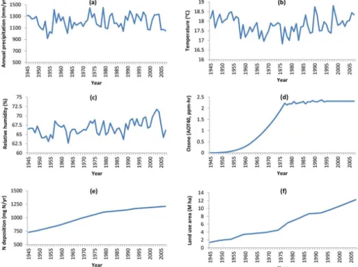
We reconstructed an 8 km resolution daily climate data set of the entire SUS from 1895 to 2005 (Figs. 2a, b, c) by integrating the daily climate pattern of the North Ameri-can regional reanalysis (NARR) (32 km resolution) data set (Mesinger et al., 2006) into the monthly PRISM (Parameter-elevation Regressions on Independent Slopes Model; 4 km resolution; 1895–present) climate data (Daly et al., 2008; prism.oregonstate.edu). A detailed description of the method is found in Zhang (2008). PRISM is a knowledge-based sys-tem to interpolate climate elements under the assumption that, for a localized region, elevation is the most important factor in the distribution of temperature and precipitation. To make predictions, PRISM dynamically calculates a lin-ear climate–elevation relationship for each DEM grid cell us-ing a movus-ing window, a procedure that smooths out signals of urbanization-induced climate changes (Daly et al., 2008). Like most reanalysis data, the surface temperatures of NARR were estimated from the atmospheric values by regional cli-mate modeling, and thus were not sensitive to changes in land surface (Kanamitsu et al., 2002). Therefore, the reanalysis data sets were used to provide information of background mate change in former UHI studies (Si et al., 2012). The
cli-mate change data from 1895 to 2005 that were reconstructed based on the PRISM and NARR data sets were used to ad-dress the background global climate change (Fig. 1; GLBC– CLM) in this study.
Ozone AOT40 data (Fig. 2d) were retrieved from a global data set developed by Felzer et al. (2004). EDGAR-HYDE 1.3 nitrogen emission data (Van Aardenne et al., 2001) were used to interpolate three maps from Dentener (2006) to generate a time-varying annual nitrogen deposition data set (Fig. 2e). Both data sources had coarse spatial resolutions (0.5–1◦) and were downscaled to 8×8 km2 using bilinear
interpolation. Due to their coarse resolutions, and because the atmospheric models that were used to generate these data sets did not consider the local urbanization effects (Felzer et al., 2005; Dentener, 2006), the AOT40 and nitrogen deposi-tion data sets represented the background global atmospheric changes in this study. The background global annual CO2
concentration was obtained from the National Oceanic and Atmospheric Administration (NOAA) (www.esrl.noaa.gov). To simulate the land use changes, the DLEM requires an-nual urban and cropland maps (1 represents urban or crop-lands; 0 represents natural vegetation). Distribution maps for cropland and urban/developed lands from 1895 to 2007 (Fig. 2f) were reconstructed by combining the contemporary land use map that was derived from NLCD2001 (Homer et al., 2007) with historical census data set for cropland, urban land, and population (Waisanen and Bliss, 2002). A detailed description can be found in Zhang et al. (2012).
Sources of other inputs, including the base maps (poten-tial vegetation, soil properties, and topographic characteris-tics, etc.) and cropland management (irrigation and fertil-ization) data sets can be found in Table S1. A detailed de-scription of the data development methodologies is found in Zhang (2008).
3.3.2 Urban-induced environmental changes
The DLEM further models the effect of urban-induced en-vironmental changes (i.e., UHI, aerosol pollutions, and in-creased CO2 and N deposition) to the urban ecosystem,
Table 2.The parameters of urban managements and urban-induced environmental changes.
Lawn managements Urban forest managements Urbanization-induced environmental changes Scenarios∗ Irrigation Litter remove Clipping interval Nitrogen fertilization % of biomass % of litter removed Elevated CO2 Reduced solar radiation Elevated NO2
(Y /N ) (Y /N ) (days) (g N m−2a−1) pruned to land fill (ppmv) due to aerosol (%) (ppmv)
SUBNZ_Cmin Y Y 5 6.4 10 % 25 % 5 −10 % 0.03
SUBNZ Y Y 10 6.8 5 % 10 % 10 −5 % 0.045
SUBNZ_Cmax Y N 15 7.3 0 % 0 % 20 0 % 0.06 ∗SUBNZrepresented the normal condition (i.e., business as usual scenario). TheSUBNZ_Cminscenario provided a conservative estimation of the urban carbon storage, while theSUBNZ_Cmaxscenario simulated the maximum carbon storage of urban/developed area.
Figure 2.Temporal patterns of major global change factors in the study region from 1945 to 2007.(a)Annual precipitation;(b)temperature; (c)relative humidity;(d)ambient ozone exposure; AOT40 is the accumulated dose over a threshold of 40 ppb during daylight hours in a month (Felzer et al., 2004);(e)annual nitrogen deposition rate;(f)urban land changes.
The urban heat island effect
The DLEM estimates the elevated temperature in urban areas (i.e., UHI, unit:◦C) with the regression model developed by
Karl et al. (1988):
UHI=α×(p)0.45, (11)
where α is a regression coefficient that varies with
sea-sons and size of urban population (p). Based on the
cli-mate records from 1219 stations in the United States, Karl et al. (1988) determined the values of α for the
maximum, minimum, and average temperature for each season in three different urban sizes (p <10 000; p∈
[10 000,100 000];p >10 000). To develop an 8 km
resolu-tion urban popularesolu-tion data set from 1945 to 2007, county-level urban population data developed by Goldewijk (2005) was divided by the area of urban/developed land to calculate the mean urban population density of each county. Then, the
urban population map for each year was developed by multi-plying the area of each urban region/patch in the NLCD 2001 land use map with the urban population density of the local county.
The elevated atmospheric CO2concentration in
urban/developed lands
Rural-urban CO2 gradient is highly variable depending on
time, location, wind direction, and distance from traffic, etc. (Idso et al., 1998, 2001, 2002; Vogt et al., 2006). The reported daily urban–rural CO2 gradient ranged from 5 (Berry and
Colls, 1990) to 66 ppmv (George et al., 2007). However, the daytime CO2 gradient that determines the CO2fertilization
CO2 concentration of the vegetated area in the center of
Phoenix, AZ was only 8 ppmv higher than the background value. According to the measurements by Clark-Thorne and Yapp (2003), the daytime CO2concentration of the urban
in-terior was averagely 5–7 ppmv higher than the rural CO2in
Dallas, TX. Garcia et al. (2012) found that the daytime sub-urban CO2concentrations were 6–16 ppmv higher than rural
levels in northern Spain. Based on these and other reports (Berry and Colls, 1990; Li et al., 2010; Rice and Bostrom, 2011), we assumed that the atmospheric CO2concentration
of an urban vegetated area is 10 ppmv higher than the back-ground value.
Urbanization-induced air pollution
Urban atmospheres have higher concentrations of nitrogen and aerosols than those in rural regions (Lovett et al., 2000; Azimi et al., 2005). In general, urban boundary layer pol-lutants are believed to reduce solar irradiance by 0–10 % in North American cities (Oke, 1979, 1982; Peterson and Stof-fel, 1980; Estournel et al., 1983). The DLEM assumed that aerosol pollutions reduce the urban solar radiation by 5 %. Urban air pollution generates high concentrations of both ozone precursors and ozone scavengers. Gregg et al. (2003) found the detrimental effects of tropospheric ozone were lower in urban than in suburban areas. Due to the uncertain-ties in urban ozone (Trusilova and Churkina, 2008), we did not consider the urbanization-induced ozone change in this study. Like atmospheric CO2, the temporal and spatial
pat-terns of urban nitrogen deposition are highly variable. Previ-ous studies indicate that the daytime atmospheric NO2
con-centration of urban and developed land usually ranges from 0.03 to 0.06 ppmv; an order higher than the value measured in rural ecosystem (Hanson et al., 1989). In this study, we used the mean value of 0.045 ppmv as the elevated urban NO2concentration.
It should be noted that these UIECs were not static but changed through time. In this study, we assumed that the rise of CO2and air pollutants in urban areas were positively
cor-related to the historical per capita fossil fuel emissions:
PLi=PLmean×f_EMS, (12)
where PLi is the urbanization-induced atmospheric change
(i.e., elevated NO2, CO2, and aerosol) in yeari; PLmeanrefers
to the mean urbanization-induced air pollution according to recent (since 1980) studies (parameters in Table 2); f_ EMSi
is the normalized fossil fuel emission factor for yeari.
f_EMSi=
EMSi
EMS1980_2000, (13)
where EMSi is the per capita annual fossil fuel emission
of the United States in year i; EMS1980_2000 denotes the
mean value between 1980 and 2000. To calculate the an-nual per capita fossil fuel emissions, we obtained the anan-nual
national fossil fuel emission data compiled by Marland et al. (2008) and the historical United States population data from the United States Census Bureau (http://www.census. gov/population/www/popclockus.html).
3.3.3 Urban managements Lawn managements
Urban lawns are irrigated, fertilized, and clipped. In the DLEM, urban lawns are irrigated whenever the soil water content is lower than 50 % of the field capacity. Since many of the United States lawns are irrigated excessively (Milesi et al., 2005), we may have underestimated the water use in irrigation. This uncertainty in irrigated water did not signifi-cantly affect the predicted C dynamics in urban lawn.
Based on the values provided by several reports in the literature, e.g., 8–9 g N m−2yr−1 (Rockwell, 1929),
5–10 g N m−2yr−1 (Thompson, 1961), 10 g N m−2yr−1
(Qian et al., 2003), 2.4–15 g N m−2yr−1 (Osmond and
Hardy, 2004), 9 g N m−2yr−1 (Law et al., 2004), and
9.7 g N m−2yr−1 (Zhou et al., 2008), the DLEM assumes
that 10 g N m−2yr−1will be the N fertilization rate for the
professionally managed lawns. This value is close to the 10.9 g N m−2yr−1 fertilization rate for the managed lawns
in the United States as estimated by Zirkle et al. (2011). In reality, however, the rates of N fertilization to lawns varied significantly from household to household in the United States (Augustin, 2007). The professionally man-aged lawn only accounts for half of the United States lawn area (Grounds Maintenance, 1996). Only half of the home lawns are fertilized in a given year (Augustin, 2007). Only 25 % of the fertilized home lawns are professionally man-aged. The remaining 75 % are managed by the home own-ers with fertilization rates ranging from 4 to 9 g N m−2yr−1.
Combining all of this information, we deduced that the an-nual N fertilization rates to United States lawns vary from 6.4 g N m−2yr−1(when 4 g N m−2yr−1is applied by home
owners) to 7.3 g N m−2yr−1(when 9 g N m−2yr−1is applied
by home owners). In the simulation, the DLEM used the av-erage value of 6.8 g N m−2yr−1for the urban lawn.
Mortality and management of urban forest
We assumed that urban trees were protected from commer-cial logging, and thus could grow very old. Large uncertain-ties exist in the mortality rate of urban trees. Field measure-ments revealed that street trees could have various mortality rates depending on their size:−2.1 to 3.0 % for trees whose DBH < 77 cm; and 5.4 % for larger trees (Nowak, 1986). Nowak (1994) assumed an annual mortality rate of 2.6 % in their urban forest modeling study. In the DLEM, the an-nual background mortality rate of urban trees ranged from 2.2 to 3.5 %, positively correlated with tree size (Nowak, 1986). Following Sitch et al. (2003), the background mor-tality is modified by light competition at the stand level. In the DLEM, forest die back will take place to maintain the foliage-projected coverage under 95 %. Urban forests have a relatively open canopy compared to rural forests, providing it an advantage to suppress light competition and support big-ger trees. The DLEM calculates the foliage-projected cover-age of urban forest based on the total area of the urban land to simulate the open canopy effect.
For simplification, we assumed rural and urban trees had the same background mortality. Unlike urban forests, rural forests in the SUS were frequently disturbed by wildfire and commercial logging (Campbell et al., 2007; Defosse et al., 2011), which were responsible for the low biomass density in the SUS forest (Birdsey, 1992). Taking the disturbances’ effect into account, the overall mortality rate of rural forest is about 10 % higher than that of protected forest (Tian et al., 2012). Following Chen (2010), we implicitly modeled the disturbances’ effect on the rural forest in the SUS by increas-ing their background mortality by 10 %.
Like lawns, urban forests may be managed by pruning and litter raking. It was found that intensive pruning might re-duce the biomass of urban trees by as much as 25 % (Nowak, 1994; Nowak et al., 2002; Escobedo et al., 2010). Unlike lawn, however, intensively managed trees, such as street trees that account for about 62 % of the managed urban forest in the United States (Kielbaso, 2008), only contribute to a small fraction (e.g., 2–4 % in Oakland, CA, and Chicago) of urban forests (Dwyer et al., 2000). Furthermore, a national survey revealed that more than 60 % of United States cities do not have urban forest management programs (Kielbaso, 2008). Even if all cities in the SUS have a forest management pro-gram, and 10 % of urban forest is street tree that accounts for 50 % of the managed forests, managed trees will only account for 20 % of urban forests. Under this assumption, about 20 %×25 %=5 % of the forest biomass was removed by pruning (Nowak, 1994; Nowak et al., 2002) (Table 2).
In some managed urban forests, a fraction of the litter (such as the litter from the pruned trees) will be removed and disposed of in a landfill. Nowak et al. (2002) assumed that only 3.7 % of the removed carbon would be released during the first 5 years, and the remaining would be perma-nently locked up in a landfill. Accordingly, the DLEM
sim-ulated the process of litter removal by allocating 1.85, 1.85, and 96.3 % of the removed litter to 1-, 10-, 100-year prod-uct pools that have turnover rates of 1, 10, and 100 years, respectively. No information about the patterns of litter man-agement is currently available for the urban/developed land in the SUS. Since the fraction of intensively managed urban forest is quite low (Dwyer et al., 2000), we assumed that only 10 % of litter will be removed and disposed of in a landfill (Table 2).
3.4 Model evaluation
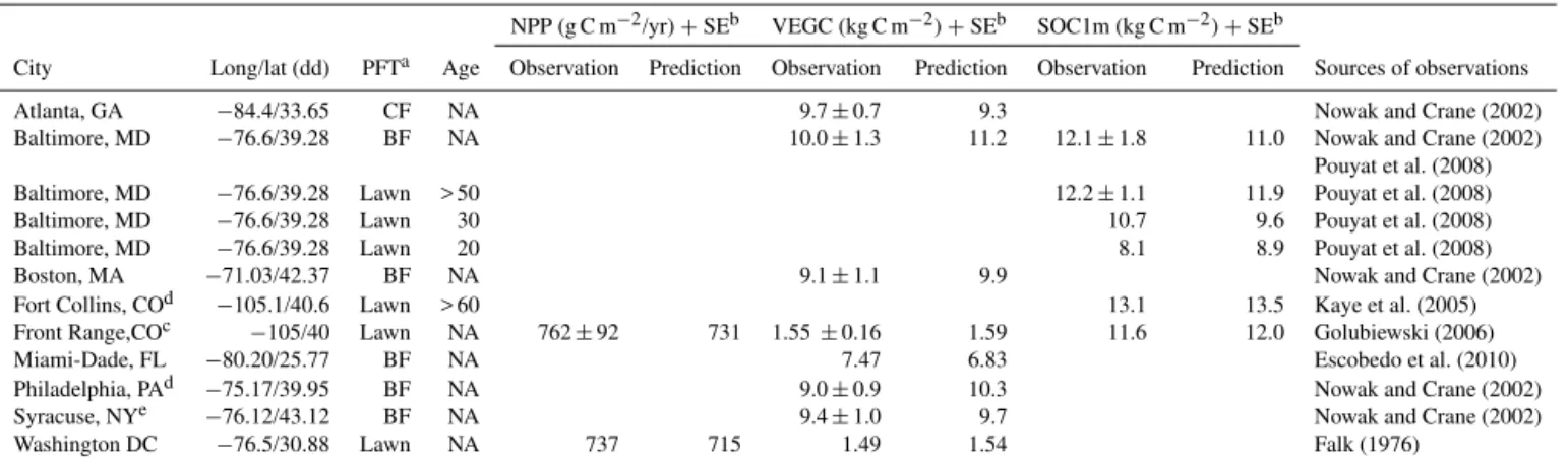
Urban ecosystem modeling is bound to large uncertainties (Churkina, 2008). Consistency between model results and field measurements is essential to establish the credibility of simulated C dynamics. Previously, we validated the DLEM simulated C and water fluxes, nitrogen cycle, soil processes, and trace gas emissions against intensively studied ecolog-ical research sites (Tian et al., 2011a, b). Because urban-ization does not change genetic characteristics of plants or fundamental mechanisms of ecological processes (Niemela, 1999), former validation results indicated that the DLEM can correctly simulate the ecosystem’s responses to multi-ple environmental stresses in urbanized areas. To evaluate the DLEM’s performance for simulating C processes in ur-ban ecosystems, we further compared model predictions with 16 field observations – including vegetation carbon (VEGC), soil organic carbon (SOC), and NPP – from 12 studies that were located in or close to the SUS (Table 4). For those stud-ies with sample variance, all of our model predictions fall into the range of 1 standard error.
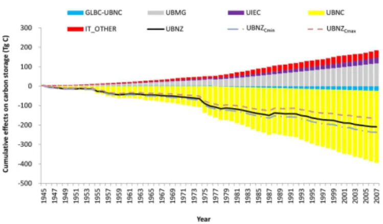
Figure 3.Cumulative effects of urbanization (UBNZ) to the car-bon dynamic of the southern United States from 1945 to 2007 and the contributions of multiple environmental drivers. UBNC is the effect of urban land conversion; GLBC–UBNC is the interac-tive effect between global environmental changes (GLBC, includ-ing changes in climate, CO2, N deposition, ozone, and landuse) and UBNC; UBMG is the management effect on the carbon dy-namic of urban vegetation (such as lawn and urban forest); UIEC is the effects due to urbanization-induced environmental changes (such as urban heat island, CO2dome effect, and elevated N deposi-tion in urban); the overall interactive effects among UBNC, GLBC– UBNC, UBMG, and UIEC are represented by IT_OTHER.
Follow-ing Zhang et al. (2012), UBNZCminand UBNZCmaxrepresent the
minimum and maximum urbanization effects, respectively, as influ-enced by uncertainties in model parameterization (Table 2).
4 Case study results
The temporal pattern of carbon dynamic during urbanization was controlled by the UBNC, which was estimated to result in about 0.37 Pg C loss from 1945 to 2007 (Fig. 3). In con-trast, the UBMGs and UIEC enhanced C storage by about 0.12 and 0.03 Pg, respectively. Factorial analysis based on numeric experiments indicated that the interactive effects be-tween global changes and urban land conversion has a nega-tive effect on C storage, causing the study area to lose about 0.02 Pg C from 1945 to 2007. The complex interactive ef-fects (i.e., IT_OTHER) among the four major types of en-vironmental changes, urban land conversion, urban manage-ments, UIECs, and GLBC–UBNC, resulted in a C seques-tration of 0.04 Pg, comparable to the effects of UIEC and GLBC–UBNC.
The effects of UEIC, urban managements, and GLBC– UBNC can be further broken down to reflect the effect of individual factors (Fig. 1). From 1945 to 2007, urban LWN management enhanced C storage by 489.9 g m−2 (the SUS
subgroup in Table 3) or 63.6 Tg in the SUS (Fig. 1), hav-ing the strongest C sequestration effect among all factors. UFMs, including direct management (Table 2) and indi-rect effects from altered disturbance regimes (e.g., protec-tion from commercial logging and wildfire), also resulted in a large C sequestration of 396.3 g m−2or 51.5 Tg. Other
fac-tors that have significant positive effects on C sequestration
included the increased N deposition (248.9 g m−2 and 32.3
Tg in the SUS) and CO2 (220.5 g m−2 and 28.6 Tg in the
SUS) in urban areas. In comparison, UHI and interactive ef-fects among UIEC factors caused 15.6 Tg (120.3 g m−2)and
16.0 Tg (123.2 g m−2)C loss from the SUS, respectively. The
interactive effect between UBNC and global change factors were smaller than other controls. While its interactions with global O3and climate change may enhance C sequestration,
interactions between UBNC and other global changes (pre-urban land use change, atmospheric CO2and N deposition
change, and the interactive effects among the global change factors) caused C loss (Fig. 1).
Because the juxtaposition of land use and ecotypes strongly influences regional patterns of urban ecosystem functions (Nowak et al., 1996), we further analyze the im-pacts of urbanization on ecosystem C density based on the dominant/potential local vegetation type (i.e., UVG; Ta-ble 3). The results indicated that urbanization had a strong negative effect on C density (−2084 g m−2)in forest areas,
only a slight negative effect on C density (−95 g m−2)in
grasslands, and a positive effect on C density (390 g m−2)
in shrubland/desert (Table 3). The C sequestration effects of UIECs and forest managements were strongest in forest ar-eas, followed by grassland and shrubland/desert areas. The interactive effects between global change and urban land conversion had a negative effect (−276 g m−2)on C density
in forest areas and a positive effect (168 g m−2)on C density
in grassland areas. Because of the large forest areas in the SUS and because of the relatively strong responses of forest C dynamics to land conversion and urban induced changes, forest areas determined the pattern of regional C dynamics in response to urbanization from 1945 to 2007 (Fig. 1; Table 3).
5 Discussion
5.1 Relative importance of the controlling factors and the implications for urban management
Although many of the factors in our urban C analysis frame-work (Fig. 1) have been individually investigated in previ-ous studies, their relative importance has rarely been com-pared. Our SUS case study showed that urban land conver-sion was by far the most important control on the regional C dynamics from 1945 to 2007, followed by urban manage-ments, overall interactive effects among major factors (i.e., IT_OTHER), urbanization-induced environmental changes, and the GLBC–UBNC interactive effect, in descending order of importance (Fig. 1). Our findings provide valuable infor-mation for regional C management. First, we found that the C loss (−2845 gC m−2)caused by urban land conversion
Table 3.Contributions of multiple environmental controls to urbanization (UBNZ) effect on carbon (C) dynamic of the forest (including needleleaf, broadleaf, mixture, and wetland forests), grass (including C3 and C4 grasslands, and grassy wetland), and arid shrubs (including shrubland and desert) ecosystems in the southern United States (SUS) from 1945 to 2007. Unit: g C m−2.
Forested Grassland Shrubland Southern
areas areas areas United States
Urbanization
(UBNZ)
ef
fects
Urban land conversion (UBNC) −2655 −1078 −303 −2845
UBNC interact with
climate change 43 33 21 39
UBNC interact with
global CO2change −89 −25 −28 −73
Interactive UBNC interact with
effects between N deposition change −86 −19 −10 −69
urban land UBNC interact with
conversion and global O3change 70 28 27 58
global changes UBNC interact with
(GLBC–UBNC) pre-urban land use change −96 12 41 −68
Interactive effects among
the global change factors −117 141 −68 −71
Overall effect of GLBC–UBNC −276 168 −18 −183
Urban heat
island effect −136 −98 −33 −120
Urbanization- Urban CO2
induced dome effect 252 155 88 221
environmental Effect from elevated
changes (UIECs) N deposition in urban areas 270 245 92 249
Interactive effects
among the UIECs −130 −131 −64 −123
Overall effect of UIECs 256 171 82 226
Urban lawn
Urban management 455 639 694 490
managements Urban forest
(UBMG) management 525 396
Overall effect of UBMG 980 639 694 886
Overall interactive effects
among UBNC, UIECs, UBMG, 411 4 −6.7 307
and GLBC–UBNC (IT_OTHER)
Overall effect of UBNZ −2084 −95 390 −1609
by assuming zero SOC in built-up areas. We estimated the SOC loss due to land conversion to be 944 gC m−2 in the
SUS, close to the estimated SOC loss (820 gC m−2)in
cen-tral Germany (Schaldach and Alcamo, 2007). Because the effect of land conversion was more than twice the combina-tion effects from all other factors (Table 3), it is preferable to preserve pre-urban C pools during land development, proba-bly by reducing soil disturbances or reserving large areas of remnant green space, rather than relying on the carbon sink in urban ecosystems to compensate for the C loss during land conversion. Like us, Escobedo et al. (2010) also suggested that preserving large trees had a larger C benefit than plant-ing young trees in the urbanized areas of the SUS. This is
Table 4.Comparison of model predictions against observed carbon pools and fluxes of urban ecosystems.
NPP (g C m−2/yr)+SEb VEGC (kg C m−2)+SEb SOC1m (kg C m−2)+SEb
City Long/lat (dd) PFTa Age Observation Prediction Observation Prediction Observation Prediction Sources of observations
Atlanta, GA −84.4/33.65 CF NA 9.7±0.7 9.3 Nowak and Crane (2002)
Baltimore, MD −76.6/39.28 BF NA 10.0±1.3 11.2 12.1±1.8 11.0 Nowak and Crane (2002)
Pouyat et al. (2008)
Baltimore, MD −76.6/39.28 Lawn > 50 12.2±1.1 11.9 Pouyat et al. (2008)
Baltimore, MD −76.6/39.28 Lawn 30 10.7 9.6 Pouyat et al. (2008)
Baltimore, MD −76.6/39.28 Lawn 20 8.1 8.9 Pouyat et al. (2008)
Boston, MA −71.03/42.37 BF NA 9.1±1.1 9.9 Nowak and Crane (2002)
Fort Collins, COd −105.1/40.6 Lawn > 60 13.1 13.5 Kaye et al. (2005)
Front Range,COc −105/40 Lawn NA 762±92 731 1.55±0.16 1.59 11.6 12.0 Golubiewski (2006)
Miami-Dade, FL −80.20/25.77 BF NA 7.47 6.83 Escobedo et al. (2010)
Philadelphia, PAd −75.17/39.95 BF NA 9.0±0.9 10.3 Nowak and Crane (2002)
Syracuse, NYe −76.12/43.12 BF NA 9.4±1.0 9.7 Nowak and Crane (2002)
Washington DC −76.5/30.88 Lawn NA 737 715 1.49 1.54 Falk (1976)
aPlant functional type (PFT); CF denotes coniferous forest; BF denotes deciduous forests.
bNPP: net primary productivity; VEGC: vegetation carbon; SOC1m: soil organic carbon (0–1 m). Table 1 values (root NPP:NPP, root C:VEGC365, C:Biomass) were used to convert
the aboveground NPP and biomass to total NPP and VEGC. By assuming that 53 % of SOC of grassland is located in the upper 30 cm (Jobbagy and Jackson, 2000), we calculated the SOC of lawns to 1 m for those studies only measuring top 30 cm.
cIntensively managed sites. 23 samples. Two tailed Student’sttest indicated differences between model predictions and observations were not significant (90 % level).
Intensively managed lawn: annual N fertilization rate=11 g N m−2yr−1; clipped litter left on site.
dThe species composition of the northern forest is not the same as that of the southern forest. Before conducting simulations in NY and PA, we estimated/calibrated the
physiological parameters of the BF functional type against the intensively studied Harvard Forest LTER site. For other cities and the regional simulations in the SUS, we used the parameters, which were developed based on the studies in the Duke Forest.
Secondly, our study showed that the urban management ef-fects have compensated for nearly one-third of the C loss due to land conversion from 1945 to 2007 in the SUS. Therefore, urban C sequestration can be enhanced through improved management practices (e.g., irrigation and fertilization) and targeted use of vehicles and machinery with least associated C emissions. According to Milesi et al. (2005), the urban lawns in the United States had a mean C sequestration rate of 37–104 g C m−2a−1. Similarly, Townsend-Small and
Cz-imczik (2010) found the C sink of managed lawns in Irvine, CA to be 140 g C m−2a−1. Zirkle et al. (2011) estimated that
lawn management increased the SOC of the United States home lawn by 78.5–79.5 g C m−2a−1. These reports agreed
well with the C sequestration effect (125 g C m−2a−1) of
lawn management in the SUS, as estimated by this study. In urban ecosystem management, it is important to quantify and reduce the hidden C cost from fossil fuel CO2emitted
during maintenance (Townsend-Small and Czimczik, 2010). According to Zirkle et al. (2011), the fossil fuel C emission in maintenance currently cost 30–56 % of the C sink induced by N fertilization and irrigation in the United States home lawn (Zirkle et al., 2011). Previous studies also indicated that, if carbon-based maintenance is performed, urban forest will eventually become a C source (Nowak et al., 2002) or a weak sink (Escobedo et al., 2010). However, intensively managed trees only account for a small fraction of the urban forest in the United States (see Sect. 3.3.3 (2)). Therefore, hid-den C cost from tree maintenance should be relatively small at regional scale. It is worth noting that there is substantial scope in reducing management-related CO2 emissions,
be-cause different equipment and maintenance techniques may have distinct C emission rates (Reid et al., 2010). For
exam-ple, it was estimated that half of the lawnmowers used by the United States homeowners belong to riding mower (Quigley, 2001), which has far larger C emissions than walk-behind mowers (Zirkle et al., 2011). By improving the efficiency of riding mowers or choosing the walk-behind mower, the maintenance C emission of urban vegetation could be signif-icantly reduced. Another possibility is to collect and utilize the 164 Tg dry biomass of lawn clippings and pruned tree twigs/limbs produced annually in the managed urban ecosys-tem in the United States for bioenergy production (Springer, 2012). Finally, well-managed urban vegetation can also in-directly reduce the C emission with its shading and cooling effects (Akbari et al., 1992).
2007; Defosse et al., 2011). Based on a literature review (see Sects. 3.2 and 3.3.3), we estimated that the overall mortal-ity rate (considering both the background mortalmortal-ity and the disturbance effect) of rural forest is about 10 % higher than that of urban forest (assuming zero disturbance from fire or commercial logging in urban areas) in SUS. Our simulation showed that the effect of management and altered distur-bance regimes together resulted in a C sink of 51.5 Tg in the SUS urban forest, stronger than the effect from urbanization-induced environmental changes. Because of direct manage-ment, such as pruning negatively affected C storage in our model simulation, the C sink can be attributed to the altered disturbance regime; a potentially important mechanism that should be further investigated in future study.
Fourthly, our study, as well as others (Ziska et al., 2004; Shen et al., 2008; Trusilova and Churkina, 2008), indicated that the UIECs had complex impacts on C dynamics, with an overall effect that promoted NPP and C sequestration. We found that urban heat island could induce C emissions, while the elevated urban nitrogen deposition and CO2
con-centration could enhance C sequestration in the SUS (Fig. 1). Our findings agreed well with the reported pattern in a Eu-rope urbanization study (Trusiloa and Churkina, 2008). Both studies found that the urban nitrogen deposition effect was stronger than the urban CO2effect, and that the urban CO2
effect was much (100 to 200 %) stronger than the UHI effect. Because these UIEC factors generally have a “dome” pattern that peaks at the city center and gradually levels off along urban–rural gradient (Idso et al., 1998), it is advisable to ar-range green spaces close to the city center to maximize their C sequestration capacity. The distinct responses from differ-ent vegetation types to urbanization should also be taken into consideration. Shen et al. (2008) suggested grass to be more sensitive to the urban CO2dome effect than desert shrub. We
found that the carbon sink effect of UEIC decreased, while the carbon sink effect of lawn managements increased, in the sequence of forest, grass, and shrub areas (Table 3). There-fore, in the forested areas, it is recommendable to improve landscape design (such as arranging green spaces close to the city center) to maximize the UIEC effect, while, in the arid shrubland areas, the focus should be put on improving urban managements to enhance C sequestration.
5.2 Complex interactive effects among factors
One of the major uncertainties in urban C dynamic is from the interactive effects among environmental factors, which could have strong ecological impacts, sometimes even de-termining the direction of the overall ecosystem C balance (Shen et al., 2008; Tian et al., 2011b). However, many former urban studies overlooked the interactive effects and assumed the effects of multiple factors to be additive (e.g., Zirkle et al., 2011). Our case study found that the overall interactive effects of the major control factors could increase C seques-tration in the SUS by about 39.9 Tg, larger than the effect of
urbanization-induced environmental changes (29 Tg, Fig. 1). This C sink is mainly located in the forested areas, which, on average, gained 411 gC m−2due to the overall interactive
ef-fects of urbanization from 1945 to 2007 (Table 3). Compared to the pre-urban forests, urban trees in general had higher biomass and productivity, because they were protected (by human managements) from disturbances (such as commer-cial logging) that caused the high overall mortality rates (con-sidering both the background mortality and the disturbance effect) and low biomass of the rural forest in SUS (Bird-sey, 1992). The strong C sink due to interactions among ur-ban land conversion, managements, and UIECs indicated that these larger urban trees are more responsive to urbanization-induced environmental changes and can fix more C, a phe-nomenon confirmed by recent observations from Escobedo et al. (2010) and Stephenson et al. (2014). The underlying mechanism is related to the relatively large total leaf area of big trees. According to the Pipe model (Shinozaki et al., 1964) that controls the photosynthate allocation in woody plants, total tree leaf mass increases as the square of trunk diameter. A typical tree that experiences a 10-fold increase in diameter will therefore undergo roughly a 100-fold in-crease in total leaf mass. Larger leaf mass means the tree has higher growth potential if not limited by water and nutri-ent availability. Therefore, bigger trees are more sensitive to elevated CO2and N deposition in urban areas. In rural forest
stand, the high C sequestration rate of large, old trees could be offset by the intensified mortality related to light competi-tion. The urban forest, however, has a relatively open canopy, and is able to support large trees (see Sect. 3.3.3). Therefore, when a rural forest became a remnant forest in urban areas, its trees could grow bigger, faster, and were more sensitive to the increased urban CO2and N deposition because of the
urban management effect that suppressed disturbances (com-mercial logging) and light competition (Table 3).
We also found a strong interactive effect (−16 Tg) among the UIEC factors (UHI, CO2 dome, and elevated N
deposi-tion), comparable to the negative effects of UHI (−15.6 Tg) (Fig. 1). Unlike Trusilova and Churkina (2008), who found that the UIEC interactive effect increased C sequestration in Europe, we found that it suppresses the urban C sink in the SUS (Fig. 1). This is mainly because the two regions ex-perienced different urbanization-induced climate changes. In our simulation, urbanization will increase local surface tem-perature in the SUS, but the data of Trusilova and Churk-ina (2008) indicated significant reduction of temperature by 0.73–1.26◦C, followed by the urbanization in Europe. We
found that the UHI effect increased potential evapotranspira-tion and exacerbated the water stress in the warm temper-ate ecosystems of the urban areas in the SUS. Like Shen et al. (2008), our simulation indicated that increasing wa-ter stress suppressed elevated CO2and N deposition effects
both climate changes improved water availability and mag-nified elevated CO2and N deposition effects.
Shen et al. (2008) suggested that the effect of urbanization-induced changes are difficult to predict due to the influence of other factors, such as global climate change. Guided by the factorial analysis scheme developed in this study, for the first time, we found a way to separate the global change effects (i.e., GLBC) from the urban land conversion (i.e., UBNC) and quantify their interactions (i.e., GLBC–UBNC) (Fig. 1). We found that GLBC–UBNC had negative effects on regional C storage (−24 Tg), almost offsetting the C sink induced by UEIC (29 Tg, Fig. 1). Such an important mecha-nism, however, had been overlooked in previous studies. The interaction between UBNC and different global change fac-tors had different effects on C dynamics. In general, GLBC– UBNC would have a negative impact on C storage if the global change factor enhanced the ecosystem C sequestra-tion. This is because the lands converted to impervious sur-face are no more responsive to global change. For example, elevated CO2 and N deposition in atmosphere stimulate C
sequestration. After a pre-urban ecosystem is converted to an impervious surface, the related C sinks (in response to CO2
fertilization) disappear. Therefore, the interactive effects be-tween urban land conversion and changes in global CO2and
N deposition seem to have a negative effect on C sequestra-tion (Fig. 1).
6 Conclusions
Urbanization involves complex changes in land structure and multiple environment factors, whose effects should not be treated independently. As urban land cover and human pop-ulation continue increasing rapidly across the globe, it is im-portant to investigate the individual effects of and complex interactions among multiple factors on the ecosystem struc-ture and processes in urbanized lands. Our case study re-vealed how the C dynamics in the 1.2×10⁵km2urbanized areas of the SUS were influenced by multiple environmental factors during the period 1945–2007. And the numeric exper-imental design and the factorial analysis schemes proposed in this study could be applied in other regions. Such efforts as the one reported here not only improve our understanding of the complex effects of urbanization on regional C dynamics, but also provide a quantitative approach for assessing the ef-fectiveness of landscape design in urbanized areas and urban development strategies.
The Supplement related to this article is available online at doi:10.5194/bg-11-7107-2014-supplement.
Acknowledgements. This study has been supported by the NSFC program (no. 31170347), the “Hundred Talents Program” of the Chinese Academy of Sciences (granted to Chi Zhang), NASA Carbon Monitoring System Program (NNX14AO73G), and the NASA IDS Program (NNX10AU06G, NNG04GM39C). We would like to thank the editor and reviewers for their valuable comments and advice.
Edited by: F. Carswell
References
Akbari, H., Davis, S., Dorsano, S., Huang, J., and Winnett, S. (Eds.): Cooling Our Communities: A Guidebook on Tree Plant-ing and Light-Colored SurfacPlant-ing, U. S. Environmental Protec-tion Agency, Office of Policy Analysis, Climate Change Divi-sion, 27–43, 1992.
Alberti, M.: The effects of urban patterns on ecosystem function, Int. Regional Sci. Rev., 28, 168–192, 2005.
Alig, R. J., Kline, J. D., and Lichtenstein, M.: Urbanization on the US landscape: looking ahead in the 21st century, Landscape Ur-ban Plan., 69, 219–234, 2004.
Augustin, B. : Perception vs Reality: How much nitrogen do home-owners put on their lawn? In Annual Meeting Abstracts [CD-ROM], ASA, CSSA, and SSSA, Madison, WI., 2007.
Azimi, S., Rocher, V., Muller, M., Moilleron, R., and Thevenot, D. R.: Sources, distribution, and variability of hydrocarbons and metals in atmospheric deposition in an urban area (Paris, France), Sci. Total Environ., 337, 223–239, 2005.
Awal, M. A., Ohta, T., Matsumoto, K., Toba, T., Daikoku, K., Hat-tori, S., Hiyama, T., and Park, H.: Comparing the carbon seques-tration capacity of temperate deciduous forests between urban and rural landscapes in central Japan, Urban For. Urban Gree., 9, 261–270, 2010.
Bartlett, M. D. and James, I. T.: A model of greenhouse gas emis-sions from the management of turf on two golf courses, Sci. Total Environ., 409, 1357–1367, 2011.
Berry, R. D. and Colls, J. J.: Atmospheric carbon dioxide and sul-phur dioxide on an urban/rural transect-I, Continuous measure-ments at the transect ends, Atmos. Environ., 24A, 2681–2688, 1990.
Birdsey, R. A.: Carbon storage for major forest types and regions in the conterminous United States, in: Forests and Global Change, Volume Z: Forest Management Opportunities for Mitigating Car-bon Emissions, edited by: Sampson, R. L. and Hair, D., Ameri-can Forests, Washington, DC, 1–26, 1996.
Buyantuyev, A., Wu, J., Gries, C., and Adger, W. N.: Multiscale analysis of the urbanization pattern of the Phoenix metropolitan landscape of USA: time, space and thematic resolution, Land-scape Urban Plan., 94, 206–217, 2010.
Campbell, J., Donato, D. C., Azuma, D., and Law, B.: Py-rogenic carbon emission from a large wildfire in Ore-gon, United States, J. Geophys. Res.-Biogeo., 112, G04014, doi:10.1029/2007JG000451, 2007.
ter-restrial carbon sources and sinks: The UK experience, Climatic Change, 42, 505–530, 1999.
Chen, G.: Effects of Disturbance and Land Management on Water, Carbon, and Nitrogen Dynamics in the Terrestrial Ecosystems of the Southern United States, PhD dissertation, Auburn University, United States, 238 pp., available at: http://etd.auburn.edu/handle/ 10415/2401 (last access: January 2014), 2010.
Churkina, G. : Modeling the carbon cycle of urban systems, Ecol. Model, 216, 107–113, 2008.
Churkina, G., Brown, D. G., and Keoleian, G.: Carbon stored in hu-man settlements: the conterminous United States, Global Change Biol., 16, 135–143, 2010.
Clark-Thorne, S. T. and Yapp, C. J.: Stable carbon isotope con-straints on mixing and mass balance of CO2in an urban atmo-sphere: Dallas metropolitan area, Texas, USA. Appl. Geochem., 18, 75–95, 2003.
Daly, C., Halbleib, M., Smith, J. I., Gibson, W. P., Doggett, M. K., Taylor, G. H., Curtis, J., and Pasteris, P. A.: Physiographically-sensitive mapping of temperature and precipitation across the conterminous United States, Int. J. Climatol., 28, 2031–2064, 2008.
Davies, Z. G., Edmondson, J. L., Heinemeyer, A. , Leake, J. R., and Gaston, K. J.: Mapping an urban ecosystem service: quantifying above-ground carbon storage at a city-wide scale, J. Appl. Ecol., 48, 1125–1134, 2011.
Day, T. A., Gober, P., Xiong, F. S., and Wentz, E. A.: Temporal pat-terns in near-surface CO2concentrations over contrasting vege-tation types in the Phoenix metropolitan area, Agr. Forest Mete-orol., 110, 229–245, 2002.
Defosse, G. E., Loguercio, G., Oddi, F. J., Molina, J. C., and Kraus, P. D.: Potential CO2 emissions mitigation through forest
pre-scribed burning: A case study in Patagonia, Argentina, Forest Ecol. Manag., 261, 2243–2254, 2011.
Dentener, F. J.: Global maps of atmospheric nitrogen deposition, 1860, 1993, and 2050,from Oak Ridge National Laboratory Dis-tributed Active Archive Center, Oak Ridge, Tennessee, USA, available at: http://daac.ornl.gov/, 2006.
Dwyer, J. F., Nowak, D. J., Noble, M. H., and Sisinni, S. M.: Con-necting people with ecosystems in the 21st century: an assess-ment of our nation’s urban forests, Gen. Tech. Rep. PNW-GTR-490. Portland, OR: U.S. Department of Agriculture, Forest Ser-vice, Pacific Northwest Research Station, 483 pp., 2000. Edmondson, J. L., Davies, Z. G., McHugh, N., Gaston, K. J., and
Leake, J. R.: Organic carbon hidden in urban ecosystems, Scien-tific Reports, 2, 963, doi:10.1038/srep00963, 2012.
Eigenbrod, F., Bell, V. A., Davies, H. N., Heinemeyer, A., Armsworth, P. R., and Gaston, K. J.: The impact of projected increases in urbanization on ecosystem services, P. Roy. Soc. B-Biol. Sci., 278, 3201–3208, 2011.
Escobedo, F., Varela, S., Zhao, M., Wagner, J. E., and Zipperer, W.: Analyzing the efficacy of subtropical urban forests in offsetting carbon emissions from cities, Environ. Sci. Policy, 13, 362–372, 2010.
Estournel, C., Vehil, R., Guedalia, D., Fontan, J., and Druilhet, A.: Observations and modeling of downward radiative fluxes (solar and infrared) in urban/rural areas, J. Climate Appl. Meteor., 22, 134–142, 1983.
Falk, J. H. : Energetics of a Suburban Lawn Ecosystem, Ecology, 57, 141–150, doi:10.2307/1936405, 1976.
Felzer, B., Kicklighter, D. W., Melillo, J. M., Wang, C., Zhuang, Q., and Prinn, R.: Effects of ozone on net primary production and carbon sequestration in the Conterminous United States using a biogeochemistry model, Tellus B, 56, 230–48, 2004.
Fenn, M. E., Haeuber, R., Tonnesen, G. S., Baron, J. S., Grossman-Clarke, S., Hope, D., Jaffe, D. A., Copeland, S., Geiser, L., and Rueth, H. M.: Nitrogen emissions, deposition, and monitoring in the western United States, BioScience, 53, 391–403, 2003. Fissore, C., Hobbie, S. E., King, J. Y., McFadden, J. P., Nelson, K.
C., and Baker, L. A.: The residential landscape: fluxes of ele-ments and the role of household decisions, Urban Ecosystems, 15, 1–18, 2012.
Garcia, M. A., Sanchez, M. L., and Perez, I. A.: Differences be-tween carbon dioxide levels over suburban and rural sites in Northern Spain, Environ. Sci. Pollut. R., 19, 432–439, 2012. George, K., Ziska, L. H., Bunce, J. A., and Quebedeaux, B.:
Ele-vated atmospheric CO2concentration and temperature across an
urban-rural transect, Atmos. Environ., 41, 7654–7665, 2007. Goldewijk, K.: Three Centuries of Global Population Growth: A
Spatial Referenced Population (Density) Database for 1700– 2000, Popul. Environ., 26, 343–367, 2005.
Golubiewski, N. E.: Urbanization increases grassland carbon pools: Effects of landscaping in Colorado’s front range, Ecol. Appl., 16, 555–571, 2006.
Gregg, J. W., Jones, C. G., and Dawson, T. E.: Urbanization effects on tree growth in the vicinity of New York City, Nature, 424, 183–87, 2003.
Groffman, P. M., Pouyat, R. V., Cadenasso, M. L., Zipperer, W. C., Szlavecz, K., Yesilonis, I. D., Band, L. E., and Brush, G. S.: Land use context and natural soil controls on plant community compo-sition and soil nitrogen and carbon dynamics in urban and rural forests, Forest Ecol. Manag., 236, 177–192, 2006.
Guilden, J. M., Smith, J. R., Thompson, L.: Stand structure of an old-growth upland hardwood forest in Overton Park, Memphis, Tennessee, edited by: Mitchell, R. S., Shevial, C. J., Leopold, D. J., in: Ecosystem Management, Rare Species and Significant Habitats, New York State Museum, Albany, 61–66, 1990. Hanson, P. J., Rott, K., Taylor, G. E., Jr., Gunderson, C. A.,
Lind-berg, S. E., and Ross-Todd, B. M.: NO2deposition to elements representative of a forest landscape, Atmos. Environ., 23, 1783– 1794, 1989.
He, C., Liu, Z., Tian, J., and Ma, Q.: Urban expansion dynamics and natural habitat loss in China: a multi-scale landscape perspective, Global Change Biol., 20, 2886–2902, doi:10.1111/gcb.12553, 2014.
Homer, C., Dewitz, J., Fry, J., Coan, M., Hossain, N., Larson, C., Herold, N., McKerrow, A., Van Driel., J. N., and Wickham, J.: Completion of the 2001 National Land Cover Database for the conterminous United States, Photogramm. Eng. Rem. S., 73, 337–341, 2007.
Houghton, R. A.: The annual net flux of carbon to the atmosphere from changes in land use 1850–1990, Tellus B, 51, 298–313, 1999.
Hutyra, L. R., Yoon, B., and Alberti, M.: Terrestrial carbon stocks across a gradient of urbanization: a study of the Seattle, WA re-gion, Global Change Biol., 17, 783–797, 2011.