MELISSA PISAROGLO DE CARVALHO
EFFICIENCY OF AMONG AND WITHIN FAMILY SELECTION IN PLANT BREEDING THROUGH SIMULATION
Thesis presented to the Federal University of Viçosa as partof the requirements for Graduation Program in Genetics and Breeding for obtaining the title of Doctor Scientiae.
VIÇOSA
MELISSA PISAROGLO DE CARVALHO
EFFICIENCY OF AMONG AND WITHIN FAMILY SELECTION IN PLANT BREEDING THROUGH SIMULATION
APPROVED: February, 27th, 2012
DEDICATION
God for always being by my side regardless of the mistakes or successes;
ACKNOWLEDGMENTS
It is a pleasure to thank the many people who made this thesis possible.
I wish to thank GOD, for helping and supporting me every single day and to give me strength in the best and worst moments.
It is difficult to overstate my gratitude to my PhD Supervisor Dr. Luiz Alexandre Peternelli, with his enthusiasm, his inspiration, his time, his intelligence and his great effort to explain things clearly and simply. Throughout my Doctor Degree period, he provided encouragement, sound advice, good teaching and lots of good ideas. For trust me and give me challenges, also for providing a stimulating and fun environment in that I learned and grew.
I wish to express my warm and sincerely thanks to Professor PhD Salvador A. Gezan, who gave me the opportunity to work with him in the School of Forest Resorce and Conservation at University of Florida. My sincerely thanks for his helping, patience, ideas and good teaching. I would have been lost without him.
I would like to thank Professor Dr. Márcio Henrique Perreira Barbosa, for his help and for giving me all field data to development my thesis.
I am especially grateful to my entire-extend family for providing a loving environmental for me, my sisters Bianca de Carvalho Hahn and her husband Silvio Cesar Hahn, Andrezza Pisaroglo de Carvalho and my brothers Tiago Pisaroglo de Carvalho and Maximiliano Pisaroglo de Carvalho, my cousin Daniela Barakat and her family, my aunt Maria de Lourdes Groth and my uncle Almiro Luis Groth for all them help, support and love.
My special thanks for my sister Andrezza Pisaroglo de Carvalho for all helping and for getting that I did not give up of my dreams.
I wish to thanks all my friends that I made in Gainesville, especially to Liz Gregg during a hard and great year.
I am grateful to my friends and my Capoeira group (Cordão de Ouro – CDO, Viçosa) for helping me get through the difficult time and all the emotional support and entertainment.
The financial support of the CNPq is gratefully acknowledged, for supporting my studies with great opportunities through of scholarship to my Doctor degree, visiting scholar and now my future Post- doc.
I am grateful to the secretary Édna and the Programa de Pós-Graduação em Genética e Melhoramento at Universidade Federal de Viçosa, for helping the departments to run smoothly and for assisting me in many different ways
BIOGRAPHY
MELISSA PISAROGLO DE CARVALHO, daughter of Carlos Alberto Marin de Carvalho (in memorian) and Elida Maria Pisaroglo de Carvalho. She has two sisters, Bianca de Carvalho Hahn, Andrezza Pisaroglo de Carvalho and two brothers Tiago Pisaroglo de Carvalho and Maximiliano Pisaroglo de Carvalho.
Born in São Leopoldo, Rio Grande do Sul, on May 11st,1975, left her hometown in September, 2000, when she began to study in Agronomy at Universidade Federal de Santa Maria (UFSM), graduating in July, 2005.
On March, 2006, she began the Programa de Pós Graduação em Produção Vegetal na Universidade Federal de Santa Maria, in Master degree, with dissertation done in February, 2008.
On March of the same year, she began the Programa de Pós Graduação em Genética e Melhoramento na Universidade Federal de Viçosa, in Doctor degree. In September, 15th, 2010, she was realized her Visiting Shcolar at University of Florida, USA, she finished in September 14th, 2011.
ÍNDICE
RESUMO ... viii
ABSTRACT ... ix
INTRODUCTION ... 1
CHAPTER 1 ... 2
GENETIC ANALYSES OF SUGARCANE TRIALS IN A BREEDING PROGRAM ... 2
RESUMO ... 2
ABSTRACT ... 3
1. INTRODUCTION ... 4
2. MATERIALS AND METHODS ... 7
2.1. Data set ... 7
2.2. Single-site analyses ... 9
2.3. Multiple-site analyses ... 10
3. RESULTS AND DISCUSSION ... 14
3.1. Single-site analyses ... 14
3.2. Multiple-site analyses ... 11
3.3. Comparison of statistical packages ... 20
4. CONCLUSIONS (AND RECOMMENDATIONS) ... 24
CHAPTER 2 ... 26
COMPARISON OF AMONG AND WITHIN SUGARCANE FAMILY SELECTION METHODS UNDER DIFFERENT GENETIC SCENARIOS ... 26
RESUMO ... 26
ABSTRACT ... 27
1. INTRODUCTION ... 28
2. MATERIAL AND METHODS ... 31
2.1. Analysis of sugarcane field trials ... 31
2.2. Field design and simulation ... 34
2.3. Statistical analysis of simulated data... 37
2.4. Selection methodologies ... 38
2.5. Simulated individual BLUP methodology ... 39
2.6.1. Differences of absolute values between the real and predicted value by both methods
BLUPI and BLUPIS ... 40
2.6.2. Correlations values ... 40
3. RESULTS AND DISCUSSION ... 41
4. CONCLUSION ... 10
GENERAL REFERENCES ... 11
RESUMO
CARVALHO, Melissa Pisaroglo, D.Sc.,Universidade Federal de Viçosa, fevereiro de 2012. Eficiência da seleção entre e dentro de famílias no melhoramento de plantas
por meio de simulação. Orientador: Luiz Alexandre Peternelli. Co-orientadores:
Márcio Henrique Pereira Barbosa e Marcos Deon Vilela de Resende.
ABSTRACT
CARVALHO, Melissa Pisaroglo, D.Sc.,Universidade Federal de Viçosa, February, 2012. Efficiency of among and within family selection in plant breeding through
simulation. Adviser: Luiz Alexandre Peternelli. Co-Advisers: Márcio Henrique Pereira
Barbosa and Marcos Deon Vilela de Resende.
INTRODUCTION
Sugarcane is a preferably alogamous plant and when grown commercially is asexually propagated (Matsuoka et al., 1999). It is a C4 plant with high photosynthetic efficiency and capacity for growing in regions of high temperatures (Machado et al., 1982; Taiz and Zeiger, 2004).
For sugarcane, the common breeding strategy has been the production of cultivars that are asexually propagated based on selection of offspring from crosses among superior parents.
Selection aims at inducing a change in the genotypic average of the population in the desired direction, through a change in allele frequencies in loci that control the traits in the selection process seeking to meet the main objectives of genetic improvement.
All breeding program want to selected families and elites clones in a short time, sometimes it can occur death of plants and wrong measurements, a tool that can help in all situation above are stochastic simulation. Other toll that also can help the sugarcane and other breeding programs are mixed models via REML/BLUP (maximum likelihood/ best linear unbias prediction with two selection methods, Individual BLUP (BLUPI) and Simulated Individual BLUP (BLUPIS). The BLUPI selected individuals inside the family, for this it need to have individual information per plot, in other hand, BLUPIS estimate the number of individuals within the family that to have to selection, all the measured for BLUPIS are in family level (plot means).
CHAPTER 1
GENETIC ANALYSES OF SUGARCANE TRIALS IN A BREEDING
PROGRAM
RESUMO
famílias separou-as em dois grupos de acordo com os valores médios das famílias e análise de componentes principais comprovou esses resultados de acordo com as estruturas morfológicas e fisiológicas das famílias.
ABSTRACT
separated in two groups according with the family average and the principal component analyses proven this group through the morphological and physiological structure.
1. INTRODUCTION
Sugarcane (Saccharum officinarum L.) has an important role in the economy due to its multiple uses. This crop can be used fresh, in the form of fodder for animal feed, or as a raw material, for manufacture of brown sugar, molasses, sugar and ethanol.
Sugarcane is grown in the tropics and subtropics, for example, Indian, China, Australia, Mexico, United States and Brazil. In the United States, sugarcane is grown commercially in Florida, Louisiana, Texas and Hawaii. In 2010, sugarcane crop totaled nearly 27.9 million tons with a value of more than US$ 991 million (NASS, 2011). In Brazil, the sugarcane production was 623 million ton per hectare. The total of 27 Brazilian states, only five states do not produce sugarcane, where São Paulo is the main producer with 54% of production (CONAB, 2011).
methods, it is possible to obtain good estimates of the genetic variance and covariance and heritability (Dudley and Moll, 1969).
The success in improving sugarcane is related to the knowledge of the genetic properties necessary for selection and genetic aspects from several traits. Knowledge of genetic variability, that can represent the potential of the population for the selection (Ramalho et al., 2004), and heritability are of great importance for the estimation of the genetic gain, success in the selection, development and deployment of new cultivars (Oliveira et al., 2010). For example, the simplest selection method can be used when the heritability is high, or more sophisticated methods are necessary when it is low, (Vencovsky e Barriga, 1992).
The most important genetic parameters to help the choice of the population and its method of selection are: the additive and dominance variance, heritability and genetic correlations. The knowledge of additive variance values allows the breeder to estimate the expected progress per cycle of selection. If the additive and dominance variances are known, one can obtain the relationship between them, which reflects the knowledge of the type of allelic interaction in controlling the character (Ramalho,1977). The genetic value of each parent is measured through the additive effects or breeding values by evaluating their offspring (Falconer & Mackay, 1996). The non-additive effects correspond to the dominance and epistasis. The dominance corresponds to the interaction of alleles at a particular locus. In contrast, epistasis effects result from the interaction between alleles at different loci.
In most of trials that used family selection, different number of seedlings per family can occur, generating an unbalanced experiment. In this situation, the best random prediction of variables, which assumed that the variance component should be estimate with high accuracy, employing the standard procedure in the context of mixed models, is restricted maximum likelihood. (Henderson, 1984; Searle et al., 1992) (REML). According with Searle et al (1992), this procedure allow the selection of individual with higher genetic values, independent of it provenance (Simeão et al.,2002). Some package that use mixed models via REML/BLUP are ASReml (Gilmour et al., 2009), Selegen – Reml/Blup (Resende, 2007), R (R Development Core Team, 2010) and SAS (Littell et al., 2006).
In sugarcane, some researchers, referring to the sexual phase, reported an individual narrow-sense heritability of 0.57 (Bressiani et al, 2007) for disease resistance, and for brix these values were 0.17 (Babu, 1990) and 0.18 (Wu et al., 1989).Results found by Hogarth et al. (1981) showed that the additive genetic variance is superior for brix, and for number, diameter and height of stalks. Others (Ferreira, 2007; Chaudhary, 2001; Bressiani, 2001; Oliveira, 2007) reported that for the variable brix the gene action is mainly additive, and according to Barbosa and Silveira (2012) and Oliveira (2007) this is the case for most economically relevant traits such as content of sugar, fiber and disease resistance. An exception is sugarcane yield where the non-additive variance is more relevant than non-additive variance (Bastos et al.,2003). They related also the no-additive genetic variance is significant for all character, except for brix and number of stalks.
using the best linear unbiased predictions (BLUPs) and for these families make the principal component analysis (PCA) to better understand the physiological and morphological characteristics.
2. MATERIALS AND METHODS
2.1. Data set
The dataset used for this work originates from the Programa de Melhoramento Genético da Cana de Açúcar (PMGCA) directed by the Federal University of Viçosa, Minas Gerais, Brazil. Data from a total of five trials were available. These trials were carried out at a breeding center at Oratórios, Minas Gerais, Brazil, located at latitude 20o25'S and longitude 42o48'W, with an altitude of 494m, an average annual rainfall of 1.250mm, an UR 64.7%, and an average minimum and maximum annual temperature of19.5 ºC and 21.8 ºC, respectively (Silva, 2009).
The trials were installed on May 2007; each consisted on a randomized complete block design (RCBD) with five blocks and 24 treatments, corresponding to a grid of 20 by 30 plots (APPENDIX – Figure I).Each experimental plot consisted of two lines spaced 1.40m with 10 plants each, equidistant at 0.5m. Each trial was composed of 22diferentfull-sib families and two controls (RB72454 and RB855046, two of the commercial varieties used in Brazil). The majority of the parents are represented in all five trials (Table 3); however, full-sib families are represented only in a single trial. The details of the collection and seedling planting procedures are described by Barbosa and Silveira (2000).Fertilization was conducted in accordance with the recommendation for the crop in the region given by Macedo et al. (2010).
longer than 1 m, and WS was obtained by weighting the complete plant and dividing by its NS only on those plants with more than five leaves. For BRIX, a single randomly selected stalk for each of the 20 plants in the plot was determined by refractometry, DS was measured using a digital caliper at ground level, and HS correspond to the height from ground level until dewlap. A summary of the trials and their measurements are presented in Table 1 and 2.
Table 1: Summary of genotypes by trial, considering a total of five trials, Oratórios,
2009.
Trial 1 Trial 2 Trial 3 Trial 4 Trial 5 Total Number of individuals 1390 1574 1790 1213 1464 7431
Number of mothers 19 21 19 18 18 95
Number of fathers 22 21 19 17 19 98
Number of families 22 22 22 22 22 110
Table 2: Average of trial for traits: number (NS), weight (WS, kg) of stalks, juice
percentage of soluble solids (BRIX,%), diameter (DS, mm) and height (HS, m) of stalks of 22 families per trial, Oratórios, 2009.
Average
Trial NS WS BRIX DS HS
1 8.60 12.12 19.42 25.18 2.49
2 7.52 10.89 19.58 25.40 2.48
3 7.86 10.61 19.98 25.26 2.54
4 8.52 11.89 19.96 25.40 2.58
2.2. Single-site analyses
After inspecting the data to detect inconsistencies and outliers, each trials was individually (i.e. single-site) analyzed using the statistical program ASReml v.3 (Gilmour et al., 2009) based on the following linear mixed model:
yijk = µ + fami+ bj + pij +eijk (1)
where, yijk corresponds to the observation belonging to the jth block, ijth plot, and ith
family; µ is the fixed overall mean; fami is the random effect of the ith family,
i=1,…,22,fami ~ N(0, ); bj is the fixed effect of the jth block, j = 1,…,5; pij is the
random effect of the ijth plot within the jth block, ij=1,…,22, pij ~ N(0,σ2p); and eijk is the
random error effect, eijk ~ N(0, σ²). All random effects, including the error term, were
considered independent and identically distributed. For this model, parental information (and pedigree) is ignored and controls were omitted from the dataset.
The total variance and cross heritability were obtained using the following expressions:
Total variance: VT = + +
Heritability of cross: ℎ =
Where corresponds to the variability of family means, which corresponds to the following expression of the genetic variance components:
= +
Here, Va and Vd correspond to the additive and dominance variance, respectively.
2.3. Multiple-site analyses
For the combined analyses considering all trials for a given trait, two linear mixed models were fitted. The first model called family model, as it only considers the family random effect, is equivalent to the one fitted for single-site analyses. On the other hand, the second model fitted partitioned the family genetic components into additive and dominance, and will be called parental model.
The family model was fitted using the following linear mixed models:
y = 1µ + X s + Z1 b + Z2 p + Z3 fam + e (2)
where, y is the vector of observation for all trials; µ is a constant representing the overall mean, s is the vector of trials fixed effects; b is the vector of random block effects within trial, with b ~ MVN (0, Ib); p is the vector of random plot effects, with p ~
MVN (0, Ip); fam is the vector of random family effects, with fam ~ MVN(0, Imf)
and e is the vector of random residual effects, with e ~ MVN (0,R), with R corresponding to a block diagonal matrix with an independent and identically distributed errors. The matrices X, Z1, Z2 and Z3 are incidence matrices that relate the
effects to the data. Also, Ix are identity matrices of the proper size. The family-by-trial
interaction term (i.e. fam×s) is not included in this model as it is confounded with fam, because none of the full-sib families were planted on more than one trial.
The parental model aims at partitioning the fam and fam×s terms into several components, based on the following expression:
+ × = ( + + ) + ( × + × )
component, and × is the interaction of a given cross with site. The above equation can also be expressed in terms of genetic components, as
+ × = 2 + 4 ! + 2 !×
where, Vaxs is the additive-by-trial interaction variance components, respectively.
The following linear mixed model was fitted for the parental model:
y = 1µ + X s + Z1b + Z2p + Z3m + Z4f + Z5 m×s + Z6 f×s + Z7mf + e (3)
where, y is the vector of observation for all trials; µ is a constant representing the overall mean, s is the vector of trials fixed effects; b is the vector of random block effects within trial, with b ~ MVN (0, Ib); p is the vector of random plot effects, with p ~
MVN (0, Ip); m and f is the random effect of male (m) and female (f), with m ~ MVN
(0,σ2mIm) and f ~ MVN (0,σ2mIm); m×s and f×s are the vector of random interaction
effects between parents and trials (overlaid), with m×s ~MVN (0, Is) and f×s ~ MVN
(0, Is); mf is the random effect of families, with mf ~ MVN(0, , Imf) and e is the
vector of random residual effects, with e ~ MVN (0,R). The matrices X, Z1, Z2, Z3, Z4, Z5, Z6and Z7 are incidence matrices that relate the effects to the data, and Ix are identity
matrices of the proper size. The R matrices correspond to a block diagonal matrix with independent and identically distributed errors, respectively.
Approximately 33% of the parents are represented in two or more trials (Table 3) for which it is possible to estimate the parental-by-site interaction (i.e. additive-by-site interaction). However, as before, the variance associated with mf contains the confounded terms of family-by-trial interaction, i.e. mf×s. Therefore, σmf2 will be
Table 3: Number of parents (mother and father), for each of the trials (diagonal) and
number of common parents among a pair of trials (off-diagonal).
Trials 1 2 3 4 5
1 39 11 11 5 5
2 39 9 2 5
3 36 7 5
4 30 12
5 35
Both, the family and parental models were fitted using ASReml (Gilmour et al., 2009) and the following parameters were calculated based on the causal components:
Additive variance: Va = 4 * σm2
Dominance variance: Vd= 4 * σmf2
Additive-by-site variance: × = 4 ∗ Total variance: VT =
2 2 2 2 2
b p m mf
σ σ σ σ+ + + +σ
Narrow sense heritability:
T a 2 a V V h = Dominance ratio: T d V V
d2 =
Heritability of cross: ℎ =
2.4. Comparison of statistical packages
In Selegen the following linear mixed model, identified by Resende (2007) as 147, was fitted:
y = 1µ + X s×b + Z1 p + Z2 fam + e (4)
where, y is the vector of observation for all trials; µ is a constant representing the overall mean, s×b is the vector of fixed effects corresponding to blocks across trials; p is the vector of random plot effects across trials; fam is the vector of random family effects, and e is the vector of random residual effects. As before, X, Z1 and Z2 are incidence
matrices that relate the effects to the data. This model is equivalent to the family model (2), but here, block effects are considered fixed. A common residual term for all trials was assumed as in (2).
2.5. Genotype selection
After performing multiple-site analyses it is possible to selects parents, crosses (i.e. families) or individual genotypes by using the family prediction according with family model (2). In this study, the top 20 families were selected, corresponding to 18.2% of 110 families evaluated. These were selected using an index with equal weight on BRIX and WS. In order to understand the physiological and morphological characteristic of these 20 selected families, principal components analysis (PCA) were done using the correlation matrix among the traits NS, HS, DS, BRIX, and WS. The first PCA analysis was done with all variables and the second one was done with the same variables as before, with the exception of HS. The exclusion of HS was to see the comportment of all others variables in terms of direction and distribution of families.
component explains the largest proportion of total variation associated with the variables of interest (Reis, 2001).
3. RESULTS AND DISCUSSION
3.1. Single-site analyses
The phenotypic and genotypic variance, together with the heritability of a cross for a single-site analyses are presented in Table4.For most trials and variables, the plot variance component (Table 4) was small or zero. The a little bit higher proportions of the total variability were found for HS with values reaching 17.3% (trial 3) and an average of 5.5%. BRIX also presented some plot variability, with an average of 2.8% across all trials. In relation of the magnitudes of the heritability of a cross, h2cross, HS
presented consistently the highest values with an average value of 14.1%, followed by BRIX and DS, with values of 7.3% and 6.6%, respectively. Almost null values of heritability were found for NS and WS for the majority of the trials. However, heritability values differed considerable from trail to trial.
Table 4:Variance component and genetics parameters of single site analyses via
ASReml for each trial and for the variables number (NS)and weight (WS) of stalks, juice percentage of soluble solids (BRIX), diameter (DS) and height (HS) of stalks of 22 families per trial, Oratórios, MG, 2009.
Trial 1
NS WS BRIX DS HS
*
1.353 3.590 0.802 0.641 0.027
0.000 0.000 0.107 0.60 0.0025
40.91 106.62 6.99 18.22 0.236
VT 42.29 110.23 7.899 19.461 0.266
h2cross 0.032 0.033 0.101 0.033 0.101
Trial 2
NS WS BRIX DS HS
0.919 4.770 0.352 1.76 0.051
0.000 0.000 0.097 0.22 0.004
30.79 91.42 6.810 18.18 0.222
VT 31.71 96.42 7.256 20.16 0.275
Trial 3
NS WS BRIX DS HS
0.451 1.050 0.240 1.560 0.019
0.346 0.280 0.202 0.000 0.050
32.96 85.26 6.56 17.81 0.220
VT 33.75 86.59 7.00 19.37 0.289
h2cross 0.013 0.012 0.034 0.081 0.066
Trial 4
NS WS BRIX DS HS
0.847 1.158 0.655 2.710 0.050
0.000 0.000 0.228 0.074 0.018
40.01 99.47 5.830 17.05 0.199
VT 40.85 100.63 6.713 19.83 0.267
h2cross 0.021 0.011 0.097 0.136 0.187
Trial 5
NS WS BRIX DS HS
0.552 0.686 0.671 1.410 0.045
0.000 0.000 0.391 0.000 0.003
38.03 97.06 6.606 18.53 0.220
VT 38.58 97.74 7.667 19.94 0.268
h2cross 0.014 0.007 0.087 0.071 0.168
*
is variance component of family; is variance component of plot; is variance component of
error;VT is total variance and h
2
corss is a heritability of crosses.
3.2. Multiple-site analyses
For multiple-sites analyses, considering the results from the family model (2) (Table 5), it was found that the design terms, i.e. block and plot, were small. When expressed as proportion of the total variability, these ranged from 0.4% to 2.3%, for blocks, and 0.0% to 2.6% for plots. The highest proportions were found for BRIX. For all traits, the residual variance components corresponded to a large portion of the total variability ranging from 83.5% to 97.3%. Therefore, in these trials there is a large within-plot variability that affects the prediction of genetic components, and these values were similar for all trials.
of 8.0% and 7.0%, respectively. In contrast, almost no genetic control was found for the traits NS and WS.
Table 5:Variance component and proportions to total variance from multiple-site
analyses of family model (2) for number (NS) and weight (WS) of stalks, juice percentage of soluble solids (BRIX), diameters (DS) and height (HS) of stalks of 110 families via ASReml, Oratorios, MG, 2009
Variance component
NS WS BRIX DS HS
Block* 0.168 0.364 0.171 0.070 0.003
Plot 0.059 0.032 0.198 0.154 0.003
Family 0.799 2.25 0.533 1.593 0.037
Error 36.56 95.98 6.564 17.96 0.219
Average 8.127 11.40 19.81 25.30 2.541
Proportions of total variance
Block 0.004 0.004 0.023 0.003 0.011
Plot 0.002 0.000 0.026 0.008 0.011
Family 0.021 0.023 0.070 0.080 0.141
Error 0.970 0.973 0.880 0.907 0.835
*
Block = Variance component of block; Plot = variance component of plot of each trial; Family = variance component of family effect and Error = variance component of error.
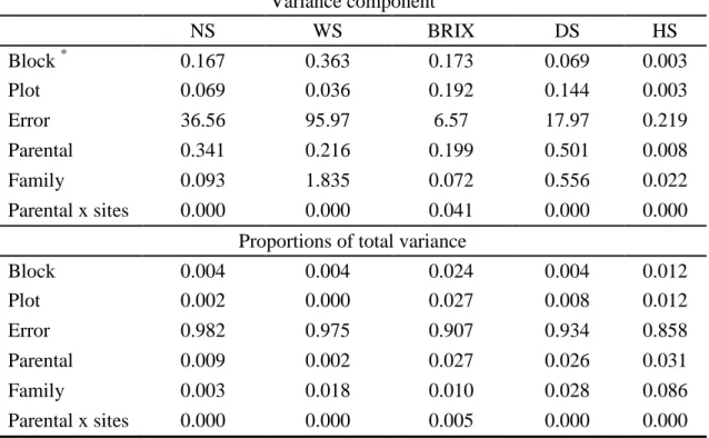
Table 6: Variance component and proportions of total variance from multiple-site
analyses of parental model (3), for number (NS) and weight (WS) of stalks, juice percentage of soluble solids (BRIX), diameters (DS) and height (HS) of stalks of 110 families via ASReml v.3, Oratórios, MG, 2009.
Variance component
NS WS BRIX DS HS
Block * 0.167 0.363 0.173 0.069 0.003
Plot 0.069 0.036 0.192 0.144 0.003
Error 36.56 95.97 6.57 17.97 0.219
Parental 0.341 0.216 0.199 0.501 0.008
Family 0.093 1.835 0.072 0.556 0.022
Parental x sites 0.000 0.000 0.041 0.000 0.000
Proportions of total variance
Block 0.004 0.004 0.024 0.004 0.012
Plot 0.002 0.000 0.027 0.008 0.012
Error 0.982 0.975 0.907 0.934 0.858
Parental 0.009 0.002 0.027 0.026 0.031
Family 0.003 0.018 0.010 0.028 0.086
Parental x sites 0.000 0.000 0.005 0.000 0.000
*
Block = Variance component of block; Plot = variance component of plot of each trial; Mother = variance component of additive effect; Family = variance component of dominance effect; Mother x sites = interaction between parents and trials, and Error = variance component of error.
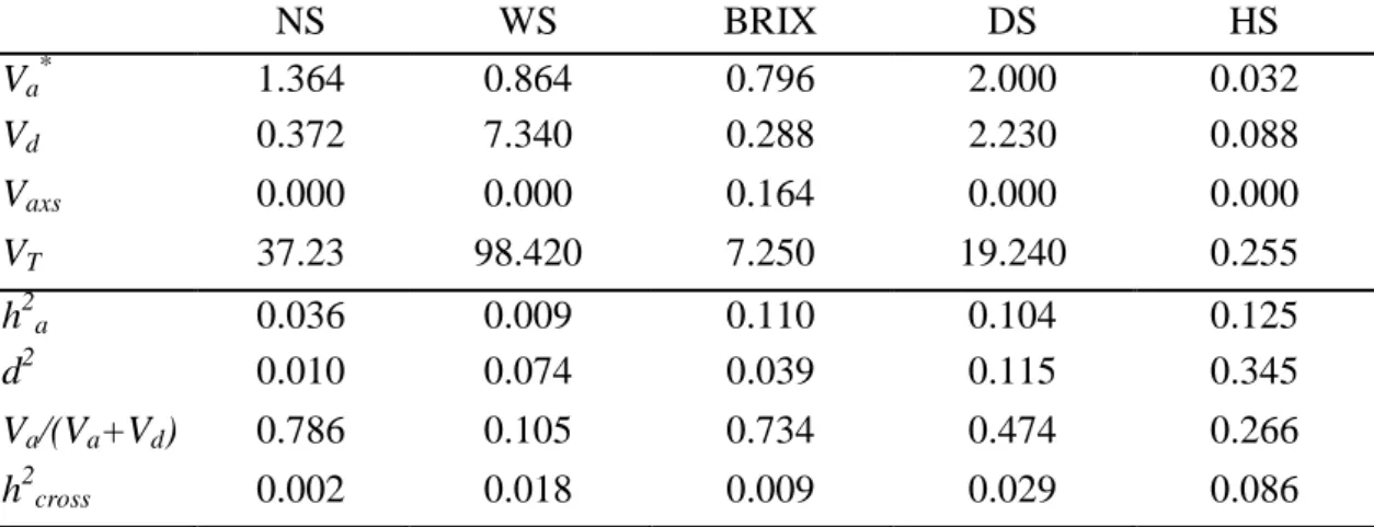
The genetic parameters estimates for all traits are presented in Table 7. The narrow-sense heritability estimates, h2a, for all variables were found to be relatively low,
ranging from 0.9% to 12.5%, with the largest values for HS, BRIX and DS and very small values for WS and NS. Therefore, it is recommended to perform parental selection on HS, BRIX and DS.
number of stalks, respectively. Martin et al (2007), estimated the heritability of cross of 0.7244 and 0.6201 for HS and DS, respectively. Silva, 2009 reported for BRIX, 0.076 of narrow-sense individual heritability and 0.63 for cross heritability.
With respect to the proportion of dominance, d2 (Table 7), which contain the dominance and dominance-by-trial interaction confounded, presented interesting values for HS, DS and WS, with a proportion as large as 34.5% for HS. For HS, DS and WS further insight through proper experiments is required in order to determine if this d2 corresponds to dominance or their interactions with site in order to determine the best selection strategy. The proportion of dominance has been reported in several studies for sugarcane. Liu et al. (2007) found a significant and higher dominance effect for WS and also a significant effect of interaction between dominance and environment.
Table 7: The average values and estimates of genetic parameters considering the five
trials for the variables number (NS) and weight (WS) of stalks, juice percentage of soluble solids (BRIX), diameter (DS) and height (HS) of stalks of 22 families via ASReml v.3, Oratórios, MG, 2009.
NS WS BRIX DS HS
Va* 1.364 0.864 0.796 2.000 0.032
Vd 0.372 7.340 0.288 2.230 0.088
Vaxs 0.000 0.000 0.164 0.000 0.000
VT 37.23 98.420 7.250 19.240 0.255
h2a 0.036 0.009 0.110 0.104 0.125
d2 0.010 0.074 0.039 0.115 0.345
Va/(Va+Vd) 0.786 0.105 0.734 0.474 0.266
h2cross 0.002 0.018 0.009 0.029 0.086
*Va= additive variance component; Vd = dominance variance component (contains dominance-by-site); × =
interaction variance component additive-by-site; VT = total variance; h2a = Narrow-sense heritability; d2 = dominance
index (contains dominance-by-site) and h2cross = cross heritability.
of2.26 %. Therefore, this interaction appears to be not relevant in these analyses, and it is expected that most parents will responds similarly across different environments.
The ratio Va/(Va+Vd) (Table 7), which denotes the relative contribution of
additive variance to total genetic variance (i.e. additive plus non-additive), was large for NS and BRIX, indicating that for these traits the genetic control is mainly additive. Equal contributions of additive and non-additive components were found for DS. In contrast, a very small ratio was found for WS, indicating almost exclusively dominance and dominance-by-site effects. The ratios obtained for NS and WS in this study agree with previous results. Matsuoka et al (1999), analyzing the relation between additive and dominance components also for sugarcane, found that for BRIX, the additive component is predominant, and for WS, the non-additive component is predominant. Also, according to Hogarth (1971), for sugarcane the variables NS and BRIX, the additive component is predominant.
Different selection strategies could be pursued for each trait according to their heritability of a cross, or the narrow-sense heritability. Hence, for a breeding program, the traits with mostly additive control could be based in early generation selection of parents, while traits with more dominance control could favor selection of families or specific crosses. In this study, the heritability of a cross, h2cross, is only relevant for HS;
therefore, it is recommended to make selection of specific crosses for this trait. Also, this trait allows for some level of gain from selection of families and parents, and BRIX and DS could be favored by selecting individual parents rather than families. Cavalcanti (1990) performed a review of literature on selection of clones and also found a high range of heritability estimates for DS and WS in studies with sugarcane.
epistasis depends on a given trait. Epistasis has been estimated in a sugarcane population for mosaic virus resistance (Xing et al., 2006), sucrose level (Richard and Henderson, 1981), and biomass traits (Hongkai et al., 2009). A study from southern China (Hongkai et al. 2009) found significant epistatic effects (additive-by-additive) for WS corresponding to a proportion of 32.1%, but no significant epistasis for the trait NS. In addition, these authors found a significant portion of epistasis-by-environment effects for WS and total biomass yield. Therefore, for the present breeding population, further studies, with appropriate experimental designs, are needed in order to understand the importance of epistasis in the traits of interest.
3.3. Comparison of statistical packages
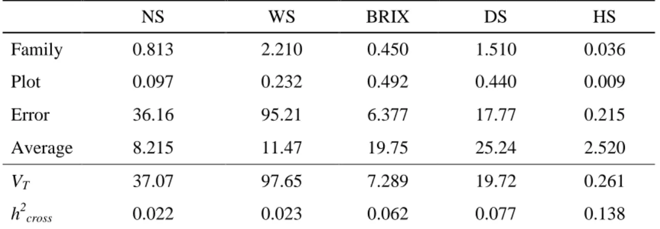
The results from fitting a family model using Selegen are presented in Table 8. In comparison with the family model fitted using ASReml (Table 5), the variance component estimates are similar for all traits. The only exception is the plot variance that resulted in larger estimates. This is probably due to the use of a different model in Selegen with blocks assumed fixed and a almost the same residual variance values for all trials. Minimal changes were noted for ℎ , with the exception of BRIX which presented smaller values, but not relevant in practice. Therefore, according to these analyses, both statistical packages provide with equivalent results. The values from
Table 8: Estimative of variance components and genetics parameters for traits: number
and weight (WS) of stalks, juice percentage of solids soluble (BRIX), diameter (DS) and height (HS) of stalks of 110 families, via model 147 from Selegen – Reml/Blup, Oratórios, MG, 2009.
NS WS BRIX DS HS
Family 0.813 2.210 0.450 1.510 0.036
Plot 0.097 0.232 0.492 0.440 0.009
Error 36.16 95.21 6.377 17.77 0.215
Average 8.215 11.47 19.75 25.24 2.520
VT 37.07 97.65 7.289 19.72 0.261
h2cross 0.022 0.023 0.062 0.077 0.138
*Family = family variance component; Plot = environmental variance between plots; Error = variance
component of error; VT = Total variance component; h
2
cross = heritability of cross and Average= average
of each trait.
3.4. Genotype selection
best genotype depends on the trait of interest. For example, family f70 had larger DS and BRIX, and families f2 and f24 had the largest WS and NS.
Table 9: Average values of all variables of group 1 and 2 for their family phenotype
and BLUP values.
Average of families
NS WS BRIX DS HS
Group 1 9.28 12.76 19.88 24.84 2.57
Group 2 7.37 11.74 20.90 26.66 2.65
Top 20 mean 8.50 12.36 20.34 25.61 2.63
Overall mean 8.20 11.44 19.76 25.23 2.52
Proportion of Gain (%)
Group 1 13.27 11.55 0.57 -1.56 1.72
Group 2 -10.04 2.63 5.77 5.67 4.89
Top 20 3.64 8.07 2.94 1.53 4.14
* Group 1 consisting of families f2, f24, f50 and f98; Group 2 consisting of families f6, f70, f89, f105.
Figure 1:Biplot from all families and traits following number of stalks (NS), diameter
of stalks (DS), weight of stalks (WS) and juice percentage of solids soluble (BRIX). The color vectors correspond to each variable and its comportment with this analysis. Red circles correspond to each family.
Principal components biplot (92.33%)
DS NS WS BRIX f87 f26 f39 f10 f24 f6 f98 f34 f76 f29 f70 f89 f2 f101 f50 f61 f38 f7 f65 f105 13.0 13.5 11.0 11.5 12.0 12.5 24 26 28 22 20.75 20.25 19.75 8 9 20.50 21.00 20.00 P C -2 (2 2 .8 4 % )
Figure 2:Biplot from all families and number of stalk (NS), height of stalks (HS),
diameter of stalks (DS), weight of stalks (WS) and juice percentage of solids soluble (BRIX). The color vectors correspond to each variable and its comportment with this analysis. Red circles correspond to each family.
4. CONCLUSIONS (AND RECOMMENDATIONS)
For single sites analysis:
-The variable height of stalks, BRIX and diameter of stalks can be used for family selection.
-Height, diameter of stalks and BRIX are good traits to be considered on breeding program in sugarcane.
- Height of stalks shows the higher heritability of crosses.
Principal components biplot (78.64%)
WS DS HS NS BRIX f87 f26 f34 f89 f24 f105 f98 f29 f76 f7 f10 f101 f50 f2 f39 f6 f70 f38 f65 f61 25 20.75 8.5 20.50 7.5 20.25 20.00 19.75 2 .8 2 .6 28 26 24 9.5 21.00 2 .5 11.0 11.5 27 12.0 12.5 13.0 8.0 13.5 2 .7 9.0 P C -2 (2 1 .3 5 % )
For multiple-site:
- Interesting non-additive effects (i.e. dominance and dominance-by-site) were found for WS, DS and HS.
- It is recommended the use of HS for family and parental selection.
- BRIX and DS should be used for parental selection rather than family selection. For PCA analyses
CHAPTER 2
COMPARISON OF AMONG AND WITHIN SUGARCANE FAMILY
SELECTION METHODS UNDER DIFFERENT GENETIC
SCENARIOS
RESUMO
ABSTRACT
1. INTRODUCTION
Sugarcane (Saccharum officinarum L.) is an alogamous species belonging to the Gramineae family (Poaceae), which is mainly asexually propagated. It is a complex polyploidy and provides raw material for the production of white sugar and alcohol (Zhou et al., 2005).
Sugarcane is an important industrial crop, totaling a production of more than 560 million tons in 2011, mainly from Brazil, Hawaii, Australia and USA. Brazil has a total of 851 million hectares or arable land, of which 6 million hectares are occupied by sugarcane crops, with a total production of about 600 million tons for the 2010/2011 harvest year (Ministério da Agricultura, 2011).
Sugarcane breeding programs aim to generate new cultivars that increase productivity and reduce economic cost (Oliveira, 2007). Sugarcane genotype selection is executed in all phases of a breeding program. It begins with parental selection followed by selection of crosses and then individuals belonging to the population, and finishes with clonal selection (Souza, 1989; Calija et al., 2001). The main objectives of these programs are the selection of potential interesting genotypes (Resende and Barbosa, 2005). Usually the measurement and selection traits are the number, height, diameter and weight of stalks, juice percentage of soluble solids (i.e. BRIX), together with production of biomass, sugar and percentage of sugar (Oliveira, 2007).
former is preferred. In phase T2, the genotypes selected from the previous phase are vegetative propagated (or 'cloned') and planted in a single plot using an augmented block design with commercial controls. For phase T3, the latest selected clones from phase T2 are now typically tested in several environments and followed through many years. These are planted as augmented blocks or randomized complete block designs. In phases T2 and T3, selection is based in choosing the best families (i.e. family selection) followed by mass selection of individuals within these families. Programs use different methods to determine the number of individuals within a family to select (e.g. simulated individual BLUP; Resende and Barbosa, 2006). Finally, during the experimental phase (FE), clones selected from phase T3 are intensively propagated and operationally evaluated in various industries and distilleries. Here, the genotypes are evaluated in several environments on large plots with three replications or more depend of number of clones and with sufficient number of harvests (Ferreira et al., 2005).
Depending on the phase, selection of individuals, families or a combination of these is used (Resende and Barbosa, 2006). Several sugarcane breeding programs have preferred family selection, as this has been shown to be superior to individual selection by providing with better genetic gains, cost of operation and resource efficiency (Stringer et al., 2011). Australian and west Indian sugarcane breeding programs use family selection (Cox and Hogarth, 1993; Kennedy and Bellamy, 1997) and in Brazil, Colombia and Argentina, a modified version of this selection is used (Bressiani et al., 2005).
generates an unbalanced experiment that requires to be analyzed using linear mixed models with the recommended statistical procedure REML (restricted maximum likelihood) allowing the simultaneous estimation of variance components and BLUP (Best Linear unbiased prediction) values for individual genotypes, families and/or parent for balance or unbalanced situations (Resende, 2004).
Sugarcane field trials are typically established with multiple plants per plot belonging to the same family. These individuals correspond to full-sibs and could be originated from sexual or asexual propagation. Yield measurements, and other traits, are obtained at the plot level, as all the individuals in a plot are harvested together. The best family is selected considering this plot level information; however, selection of the best genotypes within a family is not possible as individual measurements within a plot are not available. This could be done using within-plot mass selection, but a recommended alternative is the Simulated Individual BLUP (BLUPIS; Resende and Barbosa, 2005 and Resende, 2007). BLUPIS determines the families from which individuals (e.g. clones) that will be advanced in the program, together with the number of families and numbers individuals within a family to be selected. Resende and Barbosa (2005) report that this methodology increases the efficiency of the selection process and, compared to mass selection, it reduces costs, because in BLUPIS a smaller number of clones are advanced in the selection.
A model used for simulation must represent properly an object, system or idea, i.e. representative of the real phenomenon, and it should be flexible and easy to interpret, and the output should be comparable with the real object (Cruz, 2001).
Several simulation studies for breeding strategies have been reported. Gurgel (2004), working with autogamous plants, determined the optimal number of selected families, which can be easily extrapolated to other situations. Fernandes (2006) evaluated the efficiency of circular diallels compared to complete diallels, with respect to the estimation of general and specific combining ability. Souza et al. (2006) compared the relative efficiency for clone selection and estimation of genetic parameter based on augmented designs against randomized complete block designs. Pinto Junior (2004) used simulation for indentify the best individual and families for compose a population and them respectively clone of Eucalyptus grandis W HILL EX MIDEN. Peternelli et al. (2009) used simulation to compare the efficiency in the selection of genotypes and the quality of the estimates of the variance components and heritability for augmented block designs, duplicated augmented block designs and randomized complete block designs experiments.
The main objective of this study is to evaluate, the efficiency of the BLUPIS as a method to select sugarcane potential clones in a breeding program, through computer simulation. This will be done considering several scenarios differing in proportions of additive, dominance and epistasis variance, together with different narrow and broad sense heritabilities that mimic a range of traits of interest.
2. MATERIAL AND METHODS
2.1. Analysis of sugarcane field trials
parameters. These datasets originated from five experiments carried by the sugarcane breeding program, at Federal University of Viçosa, Minas Gerais, Brazil (see details in Chapter 1). Each experiment was carried out on May, 2007, in a randomized complete block design (RCBD) with five replication and 24 treatments. The treatments consisted of 22 full-sib families and two controls checks per trial. Therefore, the total number of treatments (or families) was 110. Each full-sib family was only represented in one experiment. For analyses, the two controls were dropped.
The phenotypic traits evaluated were: number (NS) and weight (WS, kg ha-1) of stalks, juice percentage of soluble solids (BRIX, %), and diameter (DS, cm), and height (HS, m) of stalks. For each plant, NS was measured by counting the number of stalks longer than 1 m, and WS was obtained by weighting the complete plant and dividing by its NS only on those plants with more than five leaves. For a single randomly selected stalk for each of the 20 plants in the plot, BRIX was determined by refractometry, DS was measured using a digital caliper at ground level, and HS correspond to the height from ground level until dewlap.
A multi-site analysis was performed using a linear mixed model fitted by REML/BLUP using ASReml v. 3 (Gilmour et al. 2009). The linear mixed model considered was:
y = 1µ + Xs + Z1b + Z2p + Z3m + Z4f + Z5m×s + Z6f×s + Z7mf + e (1)
where, y is the vector of observation for all trials; µ is a constant representing the overall mean, s is the vector of trials fixed effects; b is the vector of random block effects within trial, with b ~ MVN (0, Ib), p is the vector of random plot effects within trial,
with p ~ MVN (0, Ip); m and f are the vector of random parental effects
(corresponding to overlaid mother and father effects), with m ~ MVN (0, A) and f ~
MVN (0, A); m×s and f×s are the vector of random interaction effects between
(0, A⊗Is); mf is the vector of random family effects, with mf ~ MVN(0, Imf)and e
is the vector of random residual effects, with e ~ MVN (0,R). The matrices X, Z1, Z2, Z3, Z4,Z5, Z6and Z7are incidence matrices that relate the effects to the data, and Ix are
identity matrices of the proper size. The A and R matrices correspond to the numerator relationship matrix and a block diagonal matrix with independent and identically distributed errors, respectively
The results of these analyses are presented in Table 1 (more details are provided in Chapter 1). In Table 1, the summary of the genetic and environmental variance components, and other genetic parameters, are presented across all trials.
Table 1: The average values and estimates of genetic parameters, of real data via
multiple-sites analysis, considering the five trials for the variables number (NS) and weight (WS) of stalks, juice percentage of soluble solids (BRIX%), diameter (DS) and height (HS) of stalks of 110 families via ASReml v.3 parental model, Oratórios, MG, 2009.
Component NS WS BRIX DS HS
Va* 1.364 0.864 0.796 2.000 0.032
Vd 0.372 7.340 0.288 2.230 0.088
Block 0.167 0.363 0.173 0.069 0.003
Plot 0.069 0.036 0.192 0.144 0.003
Error 36.56 95.97 6.570 17.97 0.219
VT 37.23 98.42 7.25 19.24 0.255
h2a 0.036 0.009 0.110 0.104 0.125
d2 0.010 0.074 0.039 0.115 0.345
*
Va is additive variance; Vd is dominance variance component; Block is variance component of block; Plot
is variance component of plot of each trial; Error is variance component of error; VT is total variance; h
2
is
narrow-heritability and d2 is a dominance ratio.
planted in a single site. No estimate of epistasis is available from these analyses, due to the confounding of this component with the residual term.
For sugarcane, literature has reported a wide range of proportions of epistasis that depends on the trait. Hong-kai et al. (2009) found significant epistasis for WS and biomass, where the former was considerably larger than the latter. In contrast, these authors reported not significant presence of epistasis for the trait NS.
2.2. Field design and simulation
Six simulation scenarios were considered in this study, which varied according to their proportions of additive, dominance and epistasis components (Table 2). These scenarios were divided into three groups according to the magnitude of additive and non-additive variance, these were: 1) small additive and small non-additive, 2) small additive and large non-additive and, 3) large additive and small non-additive variation. In addition, within each group, different partitions of the non-additive into dominant and epistasis variance were considered: 1) with majority of dominance (D, composed by scenarios 1D and 3D) and, 2) those with majority of epistasis (I composed by scenario 1I and 3I), the scenario 2 (2D and 2I) are one exception, the values of epistasis were extrapolated and they are higher than dominance. The causal genetic components of variance were determined in proportion, for simplicity but without loss of generality, of the total variance, VT, which was set to 1. These proportions were selected, partially
Table 2: Causal genetic components of additive (Va), dominance (Vd), epistasis (Vi),
genetic variance (Vg), narrow-sense heritability (h2a) and broad sense heritability (H2) in
each scenario.
Scenarios
1D 1I 2D 2I 3D 3I
Va 0.100 0.100 0.100 0.100 0.400 0.400
Vd 0.075 0.025 0.100 0.020 0.075 0.025
Vi 0.025 0.075 0.300 0.380 0.025 0.075
Vg 0.200 0.200 0.500 0.500 0.500 0.500
h2a 0.100 0.100 0.100 0.100 0.400 0.400
H2 0.200 0.200 0.500 0.500 0.500 0.500
The experimental design generated for each of the simulated field trials consisted on typical sugarcane trial based on a RCBD with five replications and 20 rectangular plots (2 x 10 plants). The treatments consisted of 20 full-sib families without controls.
The genetic components from the scenarios defined above (Table 2), explain between 20 to 50% of the total variability. The remainder, i.e. non-genetic portion, corresponds to the variability due to design effects together with environmental noise. Based on these elements, the linear model used to simulate the data was:
yiklm = µ + pikl + gklm +eiklm (2)
where, gklm was partitioned into:
gklm= mk + fl + mfkl + c(mf)klm (3)
where, yiklm corresponds to the observation belonging to the ith block, klth plot, µ is the
fixed overall mean; pikl is the random effect of the klth plot within the ith block, ikl
=1,…,20, pikl ~ N(0, 2 p
σ ); gklm is the random effect of genotype, k = 1,…,20; l = 1,..,20
and m = 1,…,100, gklm ~ N(0,σg2) and ejkl is the random error effect, ejkl ~ N(0, σ²).The
genotype effect, is formed by a male, female, family and effect within family (individual effect), where mk is the random effect of kth male, mk ~ N(0,σ2m); fl is the
random effect of lth female, fl ~ N(0,
2
m
plot, mfkl ~ N(0,
2
mf
σ ) and c(mf)klm is the random effect of klmth individual within family
effect, c(mf)klm ~ N(0, σ2cmf). Therefore, the total genetic variance is:
2 g
σ = 2 2
m
σ +σ2mf +
2
cmf
σ . All random effects, including the error term, were assumed independent and
identically normally distributed. Therefore, parents are assumed to be unrelated.
Based in the above linear model and the values specified in Table 2, the observed variance components for the genetic population terms (i.e. male, female, family and clonal), together with the design terms (block and plot) and environmental noise used to generate the simulated datasets are specified in Table 3.
Table 3: Observed components of variance of female ( 2 f
σ ), male ( 2 m
σ ), male and family ( 2
mf
σ ), individual within family ( 2 cmf
σ ), block ( 2 b
σ ), plot ( 2 p
σ ), error (σ2) and
total ( 2 T
σ ) using for the six simulation scenarios. Scenarios
1D 1I 2D 2I 3D 3I
2
f
σ 0.025 0.025 0.025 0.025 0.100 0.100
2 m
σ 0.025 0.025 0.025 0.025 0.100 0.100
2
mf
σ 0.01875 0.00625 0.025 0.050 0.01875 0.00625
2
cmf
σ 0.13125 0.14375 0.425 0.445 0.28125 0.29375
2 b
σ 0.010 0.010 0.010 0.010 0.010 0.010
2
p
σ 0.010 0.010 0.010 0.010 0.010 0.010
2
σ 0.780 0.780 0.480 0.480 0.480 0.480
2 T
σ 1.000 1.000 1.000 1.000 1.000 1.000
variance component as specified in the Table 3. In total, 500 simulation files were generated for each of the six scenarios, in a total of 3,000 datasets available for analyses. Note that each simulation was based in an independent genetic population (i.e. 500 sets). The simulation code was implemented using the statistical software R (R Development Core Team, 2010), and the analyses were done using ASREml v.3 (Gilmour et al.,2009).
2.3. Statistical analysis of simulated data
Two statistical models were fitted to each of the datasets. First, a model based on individual plant data, called individual model, which used the following expression:
yijkl = µ + bi + pijk+ gijkl + eijkl (4)
where, yijkl corresponds to the observation belonging to the ith block, jkth plot, lth
genotype, µ is the fixed overall mean of each experiment; bi is random effect of the ith
block, bi ~ N(0, ); pijk is random effect of the jkth plot within the ith block, pijk ~
N(0, ); gijkl is random effect of the lth individual genotype within the jkth plot and ith
block, gijkl ~ N(0, $); and eijkl is the residual term, eijkl ~ N(0, ), which were assumed
identically and independently distributed. This model provides with a breeding value prediction for each of the individuals to rank and select specific genotypes. The ASReml code for extract BLUPI values was g = a + SCA + (d + i)d. Where, g is the
individual genetic effect, a is the additive effect from male and female, SCA is the specific combining ability, d is the dominance effect of families and i is the epistasis effect. This equation was used together with the pedigree file. All these are important when extract the BLUPI values because of comparison with BLUPIS values
yijk=µ + bi + mfjk + eijk (5)
where, yijk corresponds to the observation belonging to the ith block, jkth family, µ is
fixed the overall mean, bi is random effect of the ith block, bi ~ N(0, );mfjk is random
effect of the jkth family, mfjk ~ N(0, ); and eijk is the residual term, eijk ~ N(0, ),
which were assumed identically and independently distributed. All random effects were considered independent, including families. This model was used to extract the BLUPIS values through of g = 0.5(am + af) + SCA where g is the genetic effect of each family
composed of am and af which are the dominance effect from families and SCA is the
specific combining ability which give the additive effect from male and female (parents). The need of this type of model is common where the only information available is plot means (e.g. BRIX from a sample of plants). This model provides with a BLUP value for each of the families, allowing for ranking and selection of the best families. However, there are no individual predictions.
2.4. Selection methodologies
Under ideal situations, to perform forward selections an individual BLUP values (genetic or breeding value) should be available for each plant. These predictions can be used to make selections of individual plants within families or across families. Several criteria of family or individual selections can be implemented. In this study, an overall ranking of all individuals across families using the results from the individual model was obtained and the top n genotypes were selected. This methodology is called BLUPI as is based in individual BLUP values.
Alternatively, using partial information, i.e. plot means, it is possible to obtain a BLUP values for each of the families from which to make selections. Using BLUPIS, a proportion of families is determined together with the number of individuals nk to select
are chosen by mass-selection of the best genotypes within a plot based on the trait of interest or a highly correlated trait. This methodology, described by Resende and Barbosa (2006) is called BLUPIS. Further details are provided in Section 2.5. For the present study, the number of individuals to select from the top family, i.e. n0 was set to
50, which corresponds to an effective population size number of 96% of the maximum Ne of a family.
2.5. Simulated individual BLUP methodology
This methodology was development by Resende and Barbosa (2006) aiming to determine the number of individual to select within the best families, without considering individual plant phenotypes. BLUPIS does not consider those families with estimated negative genotypic effects, i.e., those with value below the average (Resende and Barbosa, 2006). The total number of individuals to be selected, nk, is determined by
the expression: nk = (gk/g0)×n0, where g0 refers to the predicted genotype value of the
best family, gk refers to the genotypic value of the kth family, and, n0 equals the number
of individuals selected from the best family (Resende, 2004; and Resende and Barbosa 2005, 2006). The determination of n0is based on the concept of effective population size
(Ne), which according to Vencovsky (1978) is expressed as: Ne = (2n0)/(n0+1)
where, n0 here is the number of individuals required to achieve the maximum percentage
2.6. Comparisons of the Methodologies
Both of the methodologies described in Section 2.4, BLUPI and BLUPIS, were compared using different statistics, such as bias and correlations.
In order to compare the selection methods, first, for each of the simulations, the top n individuals per family were determined using their real genetic values. Later, the results from the individual analyses (BLUP values) were used to perform the selection of the top n individuals to conform BLUPI method. For BLUPIS, the results from the family model identified the top families, and later, using the phenotypic values within each plot.
Initially, the top individuals per family were determined using the real genetic values, BLUPI and BLUPIS. The number of concurrencies between all possible pairs of methods was obtained, and used to obtain summary statistics.
2.6.1. Differences of absolute values between the real and predicted value by both
methods BLUPI and BLUPIS
The dataset estimated by true value, BLUPI and BLUPIS were used to obtain the three absolute difference values: First, the absolute difference between the real genetic value and BLUPI, second are between the real genetic value and BLUPIS and the third are between BLUPI and BLUPIS.
2.6.2. Correlations values
1) Between the real genetic value and BLUPI: %& '$&(&)* ;,-./0 =12 (34 5647489:;;<=>?)
34 564789:∗ ;<=>?
2) Between the real genetic value and BLUPIS: %& '$&(&)* ;,-./0@=12 (34 5647489:;;<=>?A)
34 5647489:∗ ;<=>?A
and,
3) Between BLUPI and BLUPIS: %,-./0;,-./0@ = 12 (;<=>?;;<=>?A)
;<=>?∗ ;<=>?A
Where, COV is the covariance between respective selection method and σ is the standard deviation between the respective methods. The totals of correlation were 500 for each comparison.
3. RESULTS AND DISCUSSION
Table 4 has the absolute values of the difference between the selection methodologies; the smallest differences in this case are the best results. The difference d1 showed highest average for the scenario 2I. It can be explained due to the high values of epistasis (Table 2) and low values of dominance and additives presented in this scenario. The variance component of epistasis ( * ) is high within family than among families.
The scenario 3D showed the best average for d1, and it is not very different from scenario 3I, which can be explained by present high values of additive variance and low values of epistasis. Oliveira (2007) reports, that the additive variance component is important influence on the response to selection in sugarcane.
confounded with the high values of epistasis (Table 1) from scenario 2.For scenario 3 (D and I) all results indicated smaller average values and standard deviation when compared to the other scenarios.
The results for d2, i.e. the comparison between the real genetic values with BLUPIS, was better for all scenarios than the ones obtained for d1; however, standard deviations tended to be larger than d1. This indicates that better agreements are obtained using BLUPIS but at the cost of a small increase on variability.
As expected, the average values of the differences d3 (BLUPI and BLUPIS) were lower than the other comparison of differences (d1 and d2). The average of difference ranged from 2.79 to 4.97, and the standard deviation ranged from 0.75 to 1.13. The scenario 3 (D and I) showed the lowest values of differences, it can be explained due the lower component of non-additive variance because the BLUPIS is really on BC family. This agreement between BLUPI and BLUPIS is due to the same derivation of estimators
In summary, it can be concluded that the BLUPIS methodology showed good results for all scenarios, where the best results are obtained for the situation with high additive variance and a low non-additive contribution.
Table 4: Average, standard deviation (SD) and coefficient of variation (CV%) of
absolute value of difference between the number of selection through of the real genetic value and BLUPI (d1), real genetic value and BLUPIS (d2) and between BLUPI and BLUPIS (d3).
Scenarios
1D 1I 2D 2I 3D 3I
d1 d1 d1 d1 d1 d1
Average 12.45 12.96 12.89 13.45 9.01 9.36
SD 2.04 2.08 2.01 2.01 1.94 1.84
CV(%) 16.38 16.05 15.6 14.94 21.53 19.66
d2 d2 d2 d2 d2 d2
Average 9.78 10.12 10.5 10.7 8.7 9.1
SD 2.08 2.08 2.15 2.04 2.05 2.00
CV(%) 21.27 20.55 20.48 19.07 23.64 21.97
d3 d3 d3 d3 d3 d3
Average 4.75 4.97 4.43 4.91 2.79 2.85
SD 1.12 1.09 1.12 1.08 0.78 0.75
CV(%) 23.58 21.93 25.51 21.99 27.95 26.31
To prove the efficiency of BLUPI (Table 5) the comparison of relative coincidence of number of selected between real genetic values and BLUPI were realized.
Table 5: Comparison the coincidence of number of selected between the real value and
Individual BLUP.
Scenarios
1D 1I 2D 2I 3D 3I
Average SD Range 24.6 5.2 [9.4-38] 23.9 5.4 [10.4-55] 31.6 6.5 [11-48.6] 29.6 6.1 [10.2-45.1] 34.6 5.5 [4.3-63.1] 35.1 4.9 [21.9-51.3]
The Table 6 gives the information gain between the real genetic value and BLUPI. It expresses the ratio of realized genetic gain (based on BLUPI selection), in comparison to the maximum gain that could be achieved based on selection using the real genetic values. As before, the best realized gains were found on scenario 3 (D and I). These results reinforce the idea that for high values of the additive variance and low non-additive variability, it is possible to achieve interesting gains.
Table 6: Percentage of gain of selection in comparison true value and individual BLUP
selection method.
Scenarios
1D 1I 2D 2I 3D 3I
Average 33 32 46 43 52 52
SD 0.09 0.08 0.08 0.08 0.08 0.07
Range [0.072-0.58] [-0.02-0.51] [0.2-0.65] [0.18-0.74] [0.05-0.79] [0.25-0.66]
Correlation values (Table 7) were obtained the correlation values based on the coincidence of the number of individual selected by family in each method within each scenario.
The correlation for the scenario 1D showed average of0.533, 0.593 and 0.936 respectively. Correlations between BLUPI and BLUPIS were high (average of 0.936), with little variation. The methodologies BLUPI and BLUPIS reported similar results. It can be explained because both methods use the predicted genotypic value to make the selection, where the method BLUPIS automatically eliminates the families with negative genotypic values and BLUPI method has the highest concentration of selected individuals in families with positive genotypic effect.