Interannual variations of early winter Antarctic polar stratospheric cloud formation and nitric acid observed by CALIOP and MLS

www.atmos-chem-phys.net/16/15219/2016/ doi:10.5194/acp-16-15219-2016

© Author(s) 2016. CC Attribution 3.0 License.

Interannual variations of early winter Antarctic polar stratospheric

cloud formation and nitric acid observed by CALIOP and MLS

Alyn Lambert, Michelle L. Santee, and Nathaniel J. Livesey

Jet Propulsion Laboratory, California Institute of Technology, Pasadena, California, USA

Correspondence to:Alyn Lambert (alyn.lambert@jpl.nasa.gov)

Received: 19 May 2016 – Published in Atmos. Chem. Phys. Discuss.: 13 June 2016

Revised: 17 November 2016 – Accepted: 21 November 2016 – Published: 8 December 2016

Abstract. We use satellite-borne measurements collected over the last decade (2006–2015) from the Aura Microwave Limb Sounder (MLS) and the Cloud-Aerosol Lidar with Or-thogonal Polarization (CALIOP) to investigate the nitric acid distribution and the properties of polar stratospheric clouds (PSCs) in the early winter Antarctic vortex. Frequently, at the very start of the winter, we find that synoptic-scale depletion of HNO3can be detected in the inner vortex before the first lidar detection of geophysically associated PSCs. The gener-ation of “sub-visible” PSCs can be explained as arising from the development of a solid particle population with low num-ber densities and large particle sizes. Assumed to be com-posed of nitric acid trihydrate (NAT), the sub-visible PSCs form at ambient temperatures well above the ice frost point, but also above the temperature at which supercooled ternary solution (STS) grows out of the background supercooled bi-nary solution (SBS) distribution. The temperature regime of their formation, inferred from the simultaneous uptake of ambient HNO3into NAT and their Lagrangian temperature histories, is at a depression of a few kelvin with respect to the NAT existence threshold, TNAT. Therefore, their nucleation requires a considerable supersaturation of HNO3over NAT, and is consistent with a recently described heterogeneous nu-cleation process on solid foreign nuclei immersed in liquid aerosol. We make a detailed investigation of the comparative limits of detection of PSCs and the resulting sequestration of HNO3imposed by lidar, mid-infrared, and microwave tech-niques. We find that the temperature history of air parcels, in addition to the local ambient temperature, is an important factor in the relative frequency of formation of liquid/solid PSCs. We conclude that the initiation of NAT nucleation and the subsequent development of large NAT particles capable of sedimentation and denitrification in the early winter do

not emanate from an ice-seeding process. Finally, we inves-tigate the patterns of interannual variability and compare the relative formation frequency of liquid and solid PSCs in the Antarctic lower polar stratosphere using the results of a clus-ter analysis to synthesize the combined CALIOP and MLS measurements into a relatively small number of interrelated categories.

1 Introduction

as a function of temperature. We showed that the distribu-tions of gas-phase HNO3vs. temperature combined with the independent CALIOP PSC classification (Pitts et al., 2009) provide valuable insights into the PSC formation process. Liquid STS particles exhibit well-defined equilibrium prop-erties, whereas the liquid/solid particle STS/NAT mixtures exhibit non-equilibrium properties resulting from kinetically limited growth. In this paper we expand our previous investi-gations to include the distribution of the lidar backscatter of different PSC types as a function of temperature and HNO3 uptake. We also report on the interannual variability in the Antarctic PSC seasons from 2006 to 2015.

The discrimination between different PSC types at temper-atures above the ice frost point,TICE, stemming either from the growth of STS on the background liquid supercooled bi-nary solution (SBS) or the nucleation of NAT, provides crit-ical observations enabling validation of theoretcrit-ical PSC for-mation pathways. In the case of NAT, the nucleation pro-cesses are still not understood in detail. Whether homoge-neous or heterogehomoge-neous nucleation is in force, it is the nu-cleated NAT number density that provides the key to the sub-sequent microphysical development of the NAT clouds, since rapid nucleation at high supersaturations leads to higher NAT number densities with small particle radii, whereas slow nu-cleation at low supersaturations produces low NAT number densities and allows the particles to grow to much larger sizes (Jensen et al., 2002). The homogeneous nucleation of NAT from STS and the production of large-size NAT in the 2010/2011 Arctic winter has been simulated in the SD-WACCM/CARMA PSC model (Whole-Atmosphere Com-munity Climate Model with Specified Dynamics with the Community Aerosol and Radiation Model for Atmospheres) as described by Zhu et al. (2015). In this model, homoge-neous nucleation rates were determined using the nucleation equations derived from laboratory experiments by Tabazadeh et al. (2002), with the free energy tuned by less than 10 %. The same nucleation rates were found by Zhu et al. (2016) to reproduce the observed timing of PSC formation during the Antarctic winter of 2011. In contrast, Hoyle et al. (2013) used an extension of the Zurich Optical and Microphysical box Model (ZOMM) (Luo et al., 2003) to include a new pathway of heterogeneous formation of ice and NAT on solid foreign nuclei inclusions, originating from meteoritic dust, that are assumed to be present in at least 50 % of all aerosol drops (Curtius et al., 2005).

Hoyle et al. (2013) determined that NAT can form het-erogeneously at some considerable vapor supersaturation, at temperatures well above the ice frost point, on the solid for-eign nuclei immersed in STS. Only a limited number of sur-face inhomogeneities on the foreign nuclei provide favorable active sites such that the NAT nucleation barrier is depressed sufficiently for nucleation to occur. Once the most efficient active sites have caused nucleation at a particular supersat-uration, the remaining population of STS/foreign particles have lower quality active sites that require either a higher

supersaturation to increase the nucleation rate or waiting for a longer period of time for nucleation at the same supersatu-ration to occur. Three tuning parameters are used to control the heterogeneous nucleation rate in the ZOMM model: nu-cleation barrier, nunu-cleation strength, and compatibility fac-tor. These were adjusted with consideration of the detection thresholds applied to the model results (Engel et al., 2013; Hoyle et al., 2013), to replicate successfully the CALIOP backscatter observations for a representative orbit. The tuned model was then used to facilitate intercomparisons with the CALIOP observations during December 2009 and to verify the model results for a few case studies in the Arctic (Engel et al., 2013; Hoyle et al., 2013). However, the low visibility of the NAT PSCs, as we indicated in Lambert et al. (2012), poses a detection challenge for lidar backscatter techniques, even though the accompanying HNO3sequestration in NAT can be substantial and detectable by other instruments as a decrease in the gas-phase HNO3.

PSC formation processes at play in the Arctic are clearly applicable to the Antarctic, and the recent observations from RECONCILE add support to the conclusions of our previ-ous work (Lambert et al., 2012), which highlighted the ap-pearance of synoptic-scale large particle NAT in the early Antarctic winter of 2008. Obviously, the hypotheses concern-ing the origin and microphysical characteristics of these so-called “NAT rocks” will be a challenge to validate without further in situ observations. However, the decade-long record of overlapping spaceborne CALIOP and MLS measurements presents an opportunity to develop improved algorithms for the extraction of information on PSCs and to apply new-found knowledge to the understanding of their current and future role in ozone depletion.

In Sect. 2 we review the satellite instruments and atmo-spheric measurements used in our analyses. The temperature history of an air parcel and the relation to heterogeneous nu-cleation of NAT is explored. We introduce a compact alter-native visualization to the standard graphical representation of satellite orbit plots that enables easier comprehension of several parameters plotted at multiple atmospheric levels and spanning many days of observations. In Sect. 3 we investi-gate the limits of detection of equilibrium STS and STS/NAT mixtures separately for lidar backscatter, mid-infrared ex-tinction, and uptake of HNO3from the gas phase. We also in-vestigate STS and NAT PSCs in terms of the distributions in a three-parameter space of HNO3, backscatter, and tempera-ture. We compare these with the CALIOP PSC classification scheme, which uses fixed regions within a two-parameter dis-crimination domain (depolarization vs. total backscatter). In Sect. 4 we show orbit transects and time series of co-located CALIOP and MLS data. These are used to investigate the relative formation of liquid/solid PSCs and the resulting den-itrification and renden-itrification. In Sect. 5 the early stages of formation of Antarctic PSCs at 68–21 hPa in 2009 are exam-ined using CALIOP PSC types and Lagrangian temperature history, with the inference of an initial population of sub-visible solid-particle NAT clouds superseded by a predomi-nantly liquid STS composition over a period of about a week. Finally, the interannual variability of the early Antarctic PSC seasons from 2006 to 2015 is discussed in Sect. 6.

2 Datasets and methodology

The Cloud-Aerosol Lidar with Orthogonal Polarization (CALIOP) dual-wavelength elastic backscatter lidar (Winker et al., 2009) flies on the Cloud-Aerosol Lidar and In-frared Pathfinder Satellite Observations (CALIPSO) satel-lite launched in April 2006. The Microwave Limb Sounder (MLS) is onboard the Aura spacecraft launched in July 2004. CALIPSO and Aura are part of the NASA/ESA afternoon “A-train” satellite constellation at 705 km nominal altitude and 98◦ inclination, with daily global coverage attained in 14.5 orbits. The initial A-train configuration of the CALIPSO

and Aura spacecraft from April 2006 to April 2008 resulted in an across-track orbit offset of∼200 km, with the MLS tan-gent point leading the CALIOP nadir view by about 7.5 min. Since April 2008 Aura and CALIPSO have been operated to maintain positioning within tightly constrained control boxes, such that the MLS tangent point and the CALIOP nadir view are co-located to better than about 10–20 km and about 30 s.

We derive co-located meteorological data from the God-dard Earth Observing System Data Assimilation System (GEOS-5 DAS). The 6-hourly synoptic gridded data prod-ucts (Rienecker et al., 2008) of temperatures and winds are supplied on a 540 by 361 longitude–latitude grid. The GEOS-5 data are interpolated in location and time to the MLS along-track data. Parcel temperature histories are obtained from the MLS Lagrangian Trajectory Diagnostic (LTD) dataset (Livesey et al., 2015), which consists of 15-day forward and reverse trajectories launched from a curtain of points along the Aura MLS observation track. The advection cal-culations are based on Manney et al. (1994), with wind fields and diabatic heating rates taken from the 3-hourly Modern-Era Retrospective Analysis for Research and Applications (MERRA-2) dataset (Bosilovich et al., 2015). Advances in both the GEOS-5 model and the assimilation system, in-cluding GPS Radio Occultation datasets, are included in MERRA-2. The integration uses a fourth-order Runge–Kutta scheme with a 5 min time step, and saved trajectory locations and temperatures are output every 30 min. The MLS derived meteorological products (DMPs) (Manney et al., 2007) are used where necessary to identify measurement locations that lie within the Antarctic vortex based on the potential vorticity field, sPV<−1.4, scaled in “vorticity units” (Manney et al., 1994).

2.1 CALIOP PSC data

We use the CALIOP Level-1b v3 standard data product to ex-tract information on PSCs (as documented in Lambert et al., 2012) at a 50 km horizontal by 0.5 km vertical resolution. We also use a recently released Level-2 operational dataset – L2PSCMask (v1 Polar Stratospheric Cloud Mask Product) – produced by the CALIPSO science team. The Level-2 oper-ational data consist of nighttime-only data and contain pro-files of PSC presence, composition, optical properties, and meteorological information along the CALIPSO orbit tracks at 5 km horizontal by 180 m vertical resolution.

The following three-step algorithm (using the Scientific Data Set variable names supplied with the CALIPSO Hier-archical Data Files (HDF) files) has been applied to generate the correctMIX1andMIX2classes:

INVBR=1.−1./TOTAL_SCATTERING_RATIO_532 MIX1=PSC_Composition EQ2

OR(PSC_Composition EQ3AND(INVBR LE0.2)) MIX2=PSC_Composition EQ3 AND(INVBR GT0.2) 2.2 MLS gas-phase constituents

The Microwave Limb Sounder measures thermal emission at millimeter and sub-millimeter wavelengths from the Earth’s limb (Waters et al., 2006) along the forward direction of the Aura spacecraft flight track, with a vertical scan from the sur-face to 90 km every 24.7 s. Each orbit consists of 240 scans spaced at 1.5◦ (165 km) along-track, with a total of almost 3500 profiles per day and a latitudinal coverage of 82◦S to 82◦N. The Level-1 limb radiance measurements are inverted using 2-D optimal estimation (Livesey et al., 2006) to pro-duce Level-2 profiles of atmospheric temperature and com-position. Validation of the MLS H2O and HNO3data prod-ucts and error estimations are discussed in detail by Read et al. (2007), Lambert et al. (2007), and Santee et al. (2007). Here we use the MLS version 4 (v4) data (Livesey et al., 2016) with single-profile precisions (accuracies) of 4–15 % (4–7 %) for H2O and 0.6 ppbv (1–2 ppbv) for HNO3. 2.3 Temperature history and relation to NAT

nucleation and growth processes

In this work we frequently apply a convenient temperature coordinate transformation,T−TICE, by using MLS H2O to calculate the ice frost point, in order to remove height-related variations due to changes in the H2O partial pressure (Lam-bert et al., 2012; Pitts et al., 2013). As in Lam(Lam-bert et al. (2012) we quantify the duration of exposure of an air par-cel to low temperatures by defining the temperature thresh-old exposure (TTE) as the total integrated time the air parcel is subject to synoptic-scale temperatures below the chosen threshold. We use a threshold of TICE+4 K (approximately TNAT−3.5 K) to demonstrate empirically the correlation of TTE with the uptake of HNO3 by NAT PSCs. The tem-perature history follows a diabatic back-trajectory for up to 15 days obtained from the MLS LTD dataset (Livesey et al., 2015). The TTE is the total time (in days) that an air parcel has been exposed to temperatures belowTICE+4 K since the last time the temperature fell belowTNATand remained be-lowTNATconsistently; i.e., any number of episodes of cool-ing belowTICE+4 K are accumulated provided that the air parcel has remained consistently belowTNAT. The HNO3and H2O values (for estimatingTNAT andTICE) are assumed to be constant from the start point of the back-trajectories. For typical lower stratospheric polar conditions (5 ppmv H2O,

10 ppbv HNO3, and 46 hPa), values forTICE andTNAT are 188 and 195 K, respectively. BothTICEandTNATare lowered (raised) by about 2 K at 32 hPa (68 hPa). Under denitrified conditions (5 ppbv HNO3),TNAT is lowered by about 1 K, and under dehydrated conditions (3 ppmv H2O),TICEis low-ered by about 3 K. In denitrified and dehydrated conditions, TNATis also lowered by about 3 K. TTE is a remarkably good indicator of the geographical extent of the HNO3depletion in the vortex (Lambert et al., 2012). Here, we explore the corre-spondence of TTE to NAT nucleation and growth processes. According to the development of NAT along a sample trajectory shown by Hoyle et al. (2013) in their Fig. 1, substantial nucleation begins only for temperatures below TNAT−4 K. We investigate the temperature–time domain of the nucleation process in Fig. 1, for both (a) early season unperturbed and (b) late season denitrified atmospheres, and calculate the resulting NAT number densities using the het-erogeneous nucleation scheme given in Hoyle et al. (2013). The figure serves to illustrate the general properties of NAT cloud formation, but in reality the temperature–time path is important for the modeling of specific clouds. The nucleation rate is a strong function of temperature, and the nucleated NAT shows an almost step-like transition over a narrow tem-perature range. In contrast, the variation of NAT density with exposure time is more gradual because the nucleation rate at a fixed temperature (i.e., fixed supersaturation) depends only on the integration over time. Exposure to temperatures of TNAT−2.2 K and above produces negligible NAT den-sities (<10−6cm−3), even for time durations exceeding a month, whereas exposures of∼1 day to temperatures near TNAT−4 K produce NAT densities 3 orders of magnitude greater (∼10−3cm−3_{). At lower temperatures, the NAT} sat-uration ratio is limited by uptake of HNO3 from the gas phase by STS (Luo et al., 2003), causing the curvature of the NAT density contours belowTNAT−4.5 K. Denitrifica-tion has little effect on the sharp temperature transiDenitrifica-tion, but at lower temperatures where STS forms there is a visible de-crease in the NAT number density generated for the same time duration. At nucleation, the NAT particle sizes are small and no larger than the progenitor aerosol particle (SBS or STS). Hence, considerable growth of the NAT particles is re-quired before they can be detected using remote sensing tech-niques. TTE can be viewed as a proxy for the time elapsed since nucleation occurred, i.e., as a measure of the effective growth time of the NAT particles. The NAT volume density increases gradually through sequestration of HNO3from the ambient gas phase, and the particles may not achieve their much larger equilibrium size until several days following nu-cleation.

2.4 Visual representation of satellite orbital data

col-Figure 1. (a)Calculated NAT number densities (colored shading and labeled contour lines) resulting from varying temperature ex-posure durations in an unperturbed atmosphere with 15 ppbv to-tal HNO₃. Horizontal dashed lines highlight exposures of between 1 min and 1 month. An air parcel (containing the requisite back-ground aerosol embedded with foreign nuclei) exposed to a tem-perature ofT−TNAT= −4 K for 1 day will generate 0.0012 cm−3

of nucleated NAT particles.(b)As for(a)except for a denitrified atmosphere with 5 ppbv total HNO3.

ored square is centered at the corresponding MLS profile latitude–longitude retrieval location. The along-track spac-ing is 1.5◦ (distance between centers of the squares). Note that the dimensions of the squares are not related to the MLS along-track (several hundred kilometers for HNO3) or across-track (about 10 km) resolutions. Orbit numbering (0 is the day of start orbit) is shown around the 60◦S latitude cir-cle. The color scheme indicates contrasting colors either side of 10 ppbv. Over the 10-day period (26 May to 5 June 2009, Fig. 2a and b), the HNO3values decrease and the area with values <10 ppbv is seen to increase and move eastward. Such “satellite data orbit plots” are commonly used, but they do not scale up easily for viewing multiple quantities and pressure levels over periods of the order of a month; e.g., tracking the evolution of four parameters over 20 days at four distinct atmospheric levels requires the digestion of 320 im-ages.

We present an alternative scheme, designed to improve the data visualization, with some similarities to the familiar Hov-möller diagram, but with the abscissa following selected sec-tions of the satellite orbit track rather than running along a zonal or meridional circle. Figure 2c shows the same data as in Fig. 2a, but replotted as a time-ordered sequence of the along-track points. The MLS orbit tracks are unfolded along the abscissa as a function of the along-track angle (1.5◦ is the angular spacing), where the along-track angle of 30◦ cor-responds to the closest approach of the orbit to the South Pole (at about latitude 82◦S). Also shown for convenience are the along-track distances (in kilometers) and the corre-sponding latitudes and solar zenith angles. The MLS mea-surement time (hours since start of day at 00:00 UT) is on the ordinate. The orbit numbers are given next to the right-hand ordinate. Again, the dimensions of the squares are not related to the MLS orbital track spacing or the MLS mea-surement time (each complete vertical atmospheric profile is accumulated over about 25 s). The main purpose of this compact visual representation (i.e., a sparse “raster” image) is that it enables the “raw” daily observations to be stacked into a longer time series without involving gridding onto a map projection. Note that there is a geographical data void (within 8◦of the pole; see Fig. 2a and b) that is not apparent in the raster representation. MLS looks forward in the along-track direction, so it never actually looks into the 8◦ polar cap; nor does CALIOP with its nadir view. While the low HNO3in the vortex rotates eastward in the orbit track plot, this motion translates into a time displacement in the raster plot. The ascending/descending tracks do not intersect in the raster plot and the terminator is always on the rightmost side (a feature that could be potentially useful for examining di-urnal species such as ClO).

3 Detection and classification of PSCs

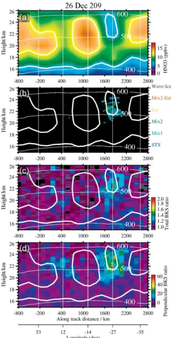
Improvements in modeling capabilities drive a commensu-rate need for a thorough evaluation of the observational as-pects of PSC research, such as biases in temperature analy-ses, derived air parcel temperature histories along trajectories and instrument measurement biases and uncertainties. This is highlighted in a specific example shown by Hoyle et al. (2013) in the Arctic on 26 December 2009 (their Fig. 7, or-bit 26_04), where they indicate that the ZOMM model pre-dicts a secondary area of NAT clouds between longitudes 12 and 53◦_{, whereas the CALIOP observations do not show}

Figure 2. (a)Polar stereographic projection of the MLS measurement locations for all orbits over the Antarctic on 2009d146 (26 May 2009). Each orbit is numbered sequentially. The square symbols denote the latitude and longitude locations of the MLS vertical profiles. The size of the squares is not representative of the along-track or across-track resolutions. The HNO3volume mixing ratio at 32 hPa is given by the

color bar.(c)The same data points are shown as a temporal raster plot. The ordinate is the time of day in hours (UT) and the abscissa is the geodetic along-track angle. The squares denote the time of day of the MLS measurement and the measurement location with respect to the closest approach of the orbit track to the South Pole. Each orbit is numbered along the right ordinate. Also shown are the along-track distance, the latitude, and the solar zenith angle. The size of the squares is not representative of the MLS integration time or the along-track resolution.(b, d)As for(a, c), except for 2009d156 (5 June 2009).

of the MLS HNO3, CALIOP L2PSCMask, and the smoothed total and perpendicular backscatter ratios. Additionally, in-spection of the MLS gas-phase HNO3identifies a coincident decrease also consistent with the location of the CALIOP PSCs (note that the ZOMM model HNO3 is not shown by Hoyle et al., 2013).

3.1 Modeled uptake of HNO3, lidar backscatter, and infrared extinction in PSCs

We model the microphysics of representative STS and NAT particle distributions according to the methodology given in Pitts et al. (2009) and Lambert et al. (2012). For the lidar scattering calculations, Mie theory is used for liquid spheri-cal particles and the T-matrix (Mishchenko and Travis, 1998)

for solid NAT particles. As we noted in Lambert et al. (2012), the NAT particle shape is an open issue, and we continue here to use a range of spheroidal shapes to illustrate the lidar sensitivity to NAT. Real refractive indices at 532 nm were assumed to be 1.43 for STS and 1.50 for NAT, with zero imaginary refractive indices for both particle types. For the mid-infrared region, complex refractive indices were ob-tained from the tabulations given by Myhre et al. (2005) for STS and Toon et al. (1994) for NAT.

Figure 3.Comparison of along-track data for the partial orbit shown by Hoyle et al. (2013) (note that thex axis is reversed here from their figure).(a)MLS HNO3showing sequestration at 12 and−27◦

longitude. (b) CALIOP PSC Mask does not show detection of PSCs at 12◦longitude.(c)Smoothed CALIOP total backscatter ra-tio.(d)Smoothed CALIOP perpendicular backscatter ratio. Solid thick white contours are the MLS HNO3isolines for 7 and 12 ppbv

HNO3. Solid thin white vertical lines are the longitude markers

shown by Hoyle et al. (2013). The detection of PSCs near 12◦ longi-tude is evident in the smoothed CALIOP perpendicular backscatter ratio along with the corresponding HNO3sequestration measured

by MLS in(a).

(Carlsaw et al., 1995). Errors in the calculations of these ref-erence temperatures arising from uncertainties in the MLS H2O and HNO3 data are estimated to be≤0.5 K for TICE and≤0.7 K forTNATin the pressure range 70–20 hPa.

SBS particles grow by condensation on cooling, first by uptake of H2O from the gas phase and, then, at sufficiently low temperatures, uptake of HNO3 occurs, forming STS at a few kelvin below the NAT point close toTSTS∼TNAT− 3.5 K (Carslaw et al., 1997; Drdla et al., 2003). In the polar stratosphere, NAT is thermodynamically stable at tempera-tures belowTNAT∼TICE+7 K, although the NAT nucleation process is still not understood in detail.

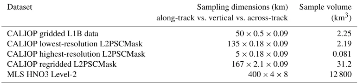
The PSC detection limits for lidar backscatter and infrared extinction are dependent on the background aerosol loading in addition to measurement noise. Under conditions of high quiescent background aerosol loadings (e.g., at times per-turbed by volcanic aerosol), a higher threshold is required to discriminate PSCs from the background. The thresholds also depend on vertical and horizontal averaging both along-track and across-track. In the case of MLS, the across-track aver-aging (i.e., the 240 GHz antenna beam width at the tangent point) is around 8 km, the vertical field of view for HNO3is a few kilometers and the along-track sampling is over several hundred kilometers. We have investigated coarser averaging of the lidar data in the along-track and vertical directions to achieve better signal-to-noise. However, the across-track av-eraging of CALIOP is only about 0.09 km, and as a result the sampling volumes of limb sounding instruments are 3 or more orders of magnitude larger. The nominal sampling vol-umes that demonstrate the much larger limb sounder sam-pling are shown in Table 1.

For illustration, here we use typical threshold levels ap-propriate for the CALIOP Level-1b v3 lidar data gridded with a 50 km by 0.5 km resolution (Lambert et al., 2012): total backscatter ratio,RT=1.25 (STS type threshold), and perpendicular backscatter,β⊥=2.5×10−6km−1sr−1(MIX

Table 1.Comparison of limb sounder and lidar sampling volumes.

Dataset Sampling dimensions (km) Sample volume along-track vs. vertical vs. across-track (km3)

CALIOP gridded L1B data 50×0.5×0.09 2.25

CALIOP lowest-resolution L2PSCMask 135×0.18×0.09 2.19 CALIOP highest-resolution L2PSCMask 5×0.18×0.09 0.081 CALIOP regridded L2PSCMask 167×2.1×0.09 31.2

MLS HNO3 Level-2 400×4×8 12 800

in STS is taken to be 1 ppbv, slightly higher than the 0.6 ppbv MLS measurement uncertainty.

3.1.1 Equilibrium STS

Figure 4a shows the temperature variation of the modeled equilibrium thermodynamic properties of STS based on the Carlsaw et al. (1995) parameterization and the calculated lidar backscatter and 12 µm infrared extinction assuming Mie theory. The calculations assume a pressure of 46 hPa, 5 ppmv H2O, and 12 ppbv total HNO3. In situ observations of the STS aerosol volume are well modeled (Carlsaw et al., 1994), as is the uptake of HNO3from the gas phase (Lam-bert et al., 2012). Uptake of HNO3 from the gas phase varies rapidly (50, 10, 1 %) over a narrow temperature range (T −TICE=2.3, 3.1, 3.9 K), and the maximum temperature derivative (−6.7 ppbv K−1) is atT−TICE=2.9 K. The theo-retical residual gas-phase HNO3, accounting for the uptake in STS, is shown in Fig. 4b as a function of the total backscatter and 12 µm infrared extinction. In a scatter plot, the observa-tions of HNO3 and backscatter (or extinction) in the pres-ence of STS are expected to lie beneath the theoretical curve, and this is investigated in Sect. 3.2. Figure 4c shows that the infrared extinction is marginally more sensitive to STS than the lidar backscatter, since the corresponding threshold equivalent condensed HNO3 contents of STS are 0.65 and 0.84 ppbv for the two measurement approaches, respectively.

3.1.2 STS/NAT mixtures

The morphology of NAT particles is still an open ques-tion, as is the compactness of the particles (Molleker et al., 2014; Woiwode et al., 2014, 2016). Light scattering stud-ies have repeatedly shown that detailed particle morphol-ogy cannot be deduced from the depolarization; e.g., Nou-siainen et al. (2012) investigated simple and complex shapes with size parameters (ratio of the particle circumference to the wavelength) in the range 2–12 and real refractive in-dices in the range 1.55–1.603 representative of silicate par-ticles, and noted similar depolarization ranges for the fifteen different shapes (regular and irregular) that were analyzed. Therefore, by analogy, the selection of a few aspect ratios for a simple spheroidal shape is sufficient to demonstrate the variations in lidar backscatter properties and to highlight

Figure 4. (a)Temperature variation relative to the frost point of the uptake of HNO3in STS (red), the calculated 532 nm lidar total

backscatter ratio,RT, (blue), and the 12 µm infrared extinction

(or-ange).(b)Gas-phase HNO3vs. 532 nm total backscatter ratio (blue)

and 12 µm infrared extinction (orange).(c)STS detection limits for lidar backscatter ratio (blue diamond) and infrared limb extinction (orange diamond) and correspondence to the uptake of HNO3 in

STS.

in Pitts et al. (2009) and Lambert et al. (2012). Previous in-vestigations (Liu and Mishchenko, 2001; Flentje et al., 2002; Lambert et al., 2012) have noted that larger depolarizations (over 60 %) result from the more nearly spherical particles in the aspect ratio rangeǫ=0.90–1.10. Recent analyses of the CALIOP data (Engel et al., 2013; Hoyle et al., 2013) have usedǫ=0.90 for NAT to improve modeling of the ob-served CALIOP depolarization range. Note that although the total backscatter is often dominated by STS, the use of a per-pendicular backscatter threshold (Lambert et al., 2012; Pitts et al., 2013), rather than an aerosol depolarization threshold, reduces the possibility of the STS signal to mask the NAT signal in STS/NAT mixtures (Biele et al., 2001).

The large particle example shown in Fig. 5a is for a NAT particle distribution with a number density NNAT= 0.001 cm−3_{and effective radiusR}

eff=6.5 µm. Note that in this example the uptake of HNO3 follows the NAT equi-librium curve until the saturation point is reached and the condensed HNO3 equals the volume in the assumed NAT particle distribution (plateau region with 4 ppbv condensed HNO3). No further uptake of HNO3 occurs until the tem-perature decreases sufficiently to allow growth of STS. This example is a crude, but not unrealistic, snapshot of a possible STS/NAT mixture at a particular time because the growth of NAT is kinetically limited (Voigt et al., 2005). A high number density of NAT nuclei would ultimately lead to a NAT distri-bution with smaller particle sizes than a low number density since the available HNO3 is spread over a large number of particles (Jensen et al., 2002). Once nucleated, a NAT parti-cle will continue to grow, provided there is sufficient HNO3 and H2O available andT < TNATsuch that the HNO3vapor pressure over NAT is supersaturated, until it attains its equi-librium size (reaching a radius of tens of microns). Gravita-tional sedimentation may cause the NAT particles to descend into a region of lower HNO3and/or rising temperature, caus-ing evaporation rather than growth. The Wegener–Bergeron– Findeisen process will cause sequestration of HNO3by NAT in a mixed-phase STS/NAT cloud at the expense of the HNO3 in the liquid STS (Voigt et al., 2005). However, if the STS forms quickly by rapid cooling, then the uptake of ambient HNO3can be predominantly into STS rather than into NAT. Growth of NAT is therefore retarded at these low tempera-tures of a few K above the frost point (Voigt et al., 2005).

The lidar detection of NAT (backscattering in the visible spectrum) is sensitive to the asphericity parameter, whereas the infrared extinction (dependent mainly on emission and therefore particle volume) is not. Hence, there are four lidar total backscatter curves corresponding to each aspect ratio in Fig. 5a, but only a single infrared extinction curve is plot-ted that is representative of all four. Likewise, the inferred uptake of HNO3 by STS/NAT as measured by microwave observations is also insensitive to particle shape (in addition, the aerosol emission is negligible in the microwave region and has no effect on the gas measurements). In the absence of an actual PSC detection, the observed reduction in

gas-Figure 5. (a)Temperature variation relative to the frost point of the uptake of HNO₃in an STS/NAT mixture (red) for a NAT num-ber density of 0.001 cm−3 and an effective radius of 6.5 µm, the calculated lidar backscatter ratio for four different particle shape aspect ratios (purple–blue), and the 12 µm infrared extinction (or-ange).(b)Condensed HNO3in NAT (red line) atT−TICE=5 K

as a function of NAT number density.(c)NAT detection limits for li-dar total backscatter ratio (blue–purple diamonds) and infrared limb extinction (orange diamond) and correspondence to the NAT num-ber density.(d)As(c), except for the lidar perpendicular backscatter coefficient only.

The theoretical condensed HNO3in NAT at a fixed tem-perature of T −TICE=5 K is shown in Fig. 5b as a func-tion of the NAT number density. At this temperature, the STS contribution to the backscatter, infrared extinction, and HNO3 uptake is negligible (see Fig. 4) and we may safely concentrate on the properties of the NAT particles alone. The temperature is about 2.5 K below the NAT existence temper-ature and about 2 K above the tempertemper-ature at which substan-tial uptake of HNO3into STS occurs. The red diamond sym-bol marks the detection threshold for 1 ppbv of HNO3 con-densed in NAT (or equivalently a 1 ppbv uptake of HNO3 from the gas phase) and corresponds to a NAT number den-sity of 2.45×10−4cm−3. In Fig. 5c we show the total lidar backscatter and infrared extinction as a function of the NAT number density. The total backscatter detection threshold (1.25) for the four particle aspect ratios corresponds to NAT number densities ranging from 4.9 to 8.4×10−4cm−3 com-pared to 1.4×10−4cm−3_{for the infrared extinction} thresh-old (kext=5×10−5km−1). For this large particle radius ex-ample, uptake of HNO3 and infrared detections are more sensitive than the lidar total backscatter. The perpendicular backscatter coefficient (Fig. 5d) is more sensitive than the to-tal backscatter to the presence of non-spherical NAT, result-ing in the detection of lower number densities rangresult-ing from 1.2 to 3.6×10−4cm−3, except for the 0.8 aspect ratio, which shows less sensitivity. Hence, operation of a lidar with an or-thogonal polarization channel can substantially improve the detection threshold for non-spherical NAT for some aspect ratios. The infrared detection is shown to be more sensitive for the large particle range, except for an aspect ratio of 0.95 for which the sensitivities are comparable.

3.1.3 Intercomparisons of PSC detection techniques

The sensitivity of different techniques employed to detect PSCs over a wide range of number densities and effective radii is illustrated with Fig. 6. Selected detection limits for CALIOP lidar, infrared limb emission, and inferred detection by the measured uptake of HNO3from the gas phase or the in situ aerosol detection of condensed HNO3in NAT are shown. Again, the calculations are for a temperatureT−TICE=5 K, since the purpose of the comparison is to show the potentially large variation in lidar backscatter response to NAT PSCs of differing asphericities. The lines in Fig. 6 mark the detec-tion limits for the various techniques and indicate the low-est NAT number density (NNAT) that can be detected for a given NAT effective radius (Reff); i.e., any combination of (NNAT, Reff) lying below a given line is below the detection limit for that particular technique. The gray shading indicates the region that is below the detection threshold for any of the techniques assuming the given variation in NAT aspect ratio. The solid (dashed) purple–blue lines correspond to the detec-tion thresholds for total backscatter (perpendicular backscat-ter) for different aspect ratios. As expected from the previ-ous section, the perpendicular backscatter is in general more

Figure 6.Intercomparison of the sensitivity of various PSC detec-tion techniques to a range of NAT number densities and effective radii at a temperature ofT−TICE=5 K, for an ambient pressure

of 46 hPa, 5 ppmv H2O, and 12 ppbv total HNO3. The purple–blue

lines indicate the limits of detection for lidar with total backscat-ter (solid) and orthogonal channel (dashed) for a range of aspect ratios (EPS). The red (green) line indicates the sensitivity of an in situ sampling instrument to 1 ppb of condensed HNO₃in NAT (aerosol density, 0.2 µm3cm−3) or the equivalent uptake from the gas phase (e.g., by a microwave limb sounder). Yellow/orange lines indicate the sensitivities in the mid-infrared for a limb sounder at two wavelengths. NAT PSCs with particle distribution characteris-tics lying within the gray shaded region are undetectable by any of the above techniques, with the assumed horizontal and vertical averaging scales given in the text.

Reff>5 µm, respectively. The near coincidence of the green dashed line and red solid line shows that a NAT volume den-sity of 0.2 µm3cm−3_{(limit of detection for MIPAS given by} Höpfner et al., 2006b) is approximately equivalent to 1 ppbv of condensed HNO3. This threshold is consistent with a pre-vious study by Höpfner (2004) that showed that large parti-cle, small number density NAT can be detected by MIPAS. The specific case studied was for a particle distribution with a 7 µm mode radius and number density 2.9×10−4cm−3, which we estimate to be equivalent to a 12 µm extinction of 1.9×10−4km−1(practically independent of the particle as-pect ratio in the infrared region).

3.2 Separation of PSC types using backscatter, HNO3, and temperature

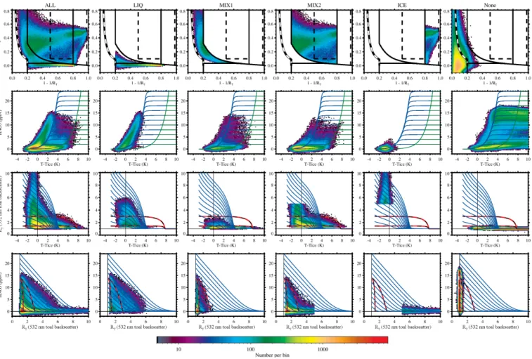
In this section we investigate the lidar PSC classification by exploring the 2-D cross sections resulting from projections of the 3-D coordinate space of temperature, HNO3, and to-tal backscatter. Here we use the CALIOP Level-1b v3 data with coincident MLS data processed as detailed in Lambert et al. (2012) for the period 10 May to 25 October 2009 in the Antarctic at 46–21 hPa. In Fig. 7 we show probability density functions (PDFs) classified according to the CALIOP PSC scheme (Pitts et al., 2009), with modifications discussed in Lambert et al. (2012) and Pitts et al. (2013), in six columns (ALL, LIQ, MIX1, MIX2, ICE, andNone) and four rows (described below). TheALLclass is the sum of the indi-vidually classified PSC components LIQ, MIX1, MIX2, and ICE. The None class represents all cases below the CALIOP detection threshold. The four rows for each column show the depolarization vs. normalized backscatter and the corresponding PDFs for the three possible combinations of pairings from the temperature, HNO3, and total backscatter coordinates in the PSC classification. Nitric acid vs. temper-ature has been shown previously by Lambert et al. (2012) and Pitts et al. (2013) (and is included for completeness), but backscatter vs. temperature and HNO3vs. backscatter are shown for the first time here.

3.2.1 Row 1: depolarization (δ) vs. normalized backscatter (1₋1/RT)

CALIOP data analysis, detection, and classification are dis-cussed in Lambert et al. (2012) and Pitts et al. (2013). The PSC classes are shown in the CALIOP depolariza-tion vs. backscatter classificadepolariza-tion diagram in the first row. Black solid lines indicate the main PSC types. Class bound-aries for MIX2-enh and wave ice (RT>50) are shown as black dashed lines, but are not differentiated here from the MIX2andICEmain classes. The classification bound-aries were originally chosen (Pitts et al., 2009) to distin-guish STS (depolarization less than 3 %), STS/NAT mix-tures (significant depolarization indicating a solid compo-nent), and ice. Note that the LIQ/MIX1class boundary is

fuzzy, and depolarization values (the ratio of the perpen-dicular to parallel backscatter) can exceed 3 % forLIQ be-cause of measurement noise even though the perpendicular backscatter component indicates below-threshold response. Similarly, theNoneclass boundary is fuzzy because of mea-surement noise. The black–white dashed line shows the the-oretical lower limit of detection as a locus of points (δ, 1−1/RT) for the chosen perpendicular backscatter thresh-old,β⊥=2.5×10−6km−1sr−1, calculated for a typical

po-lar atmosphere from the expression

RT(δ)=

1+1 δ

(β⊥−βm⊥)+βmT

1 βT

m ,

where the molecular depolarizationδmis 0.0036, the molec-ular perpendicmolec-ular backscatter componentβm⊥ is βmT1+δmδm,

the total Rayleigh scattering (both polarizations) isβ_mT, and the fractional depolarization range isδ=0. . .1. This low de-tection limit is not strictly attained in practice because of additional spatial coherence constraints that are imposed to reduce false positives to less than 0.1 % (Lambert et al., 2012). The coherence constraint results in the distribution of points in theNoneclass appearing to the right side of the black–white dashed line. All the other imposed class bound-aries are sharp, although this does not imply that the distinc-tion between these PSC types is definitive. For example, as noted in Pitts et al. (2013), theICE“arm” close to theLIQ class (normalized backscatter 0.7–0.85) is intersected by the MIX2/ICEboundary. Better separation between theMIX2 andICEclasses based on allowing for the seasonal variation in the location of the ice “arm” associated with denitrification was discussed in Pitts et al. (2013). Overall, the classification using the 2-D regions of the depolarization vs. normalized backscatter provides very good discrimination between STS and solid-particle PSCs.

3.2.2 Row 2: Gas-phase HNO3vs.T −TICE

Figure 7. CALIOP PSC type classifications and their corresponding 2-D cross-section pairs derived from the 3-D coordinate space of temperature T−TICE, HNO3, and total backscatter, RT, for 10 May to 25 October 2009. The six columns are the CALIOP PSC types

identified in the text. Blue (green) lines are theoretical calculations for total HNO3 from 2 to 24 ppbv in 2 ppbv steps for STS (NAT)

equilibrium. Red–black dashed lines are theoretical calculations for equilibrium NAT with number densities 0.001 cm−3(bottom curve) and 0.01 cm−3(top curve) and 14 ppbv total HNO3. The lower limit of detection, given by the black–white dashed line, is described in the text.

The leading edge of the HNO3gas-phase distribution for the Noneclass follows the STS uptake curve. Also visible is a separate highly denitrified branch (HNO3<5 ppbv) extend-ing to beyond 10 K above the ice frost point.

3.2.3 Row 3: total backscatter (RT) vs.T−TICE

This row shows the temperature domains corresponding to the various CALIOP PSC classes (the region of highest backscatter, RT>10, is not shown). The blue lines indi-cate the theoretical STS backscatter vs. T−TICE for gas-phase HNO3 increasing from 2 to 24 ppbv in 2 ppbv steps. Note that the current depolarization/backscatter classifica-tion scheme does not use temperature as a discriminant. Backscatter vs. temperature is only used in the CALIOP classification scheme to determine daily detection thresholds (Pitts et al., 2009). TheLIQclass shows a rapid increase in total backscatter nearT−TICE=3.5 K (i.e.,TSTSis located at the point the blue curves join the abscissa). There is a thin tail which does not reach out as far as TNAT(located at the

spa-tial resolution than is shown here. At the highest backscatter values there is an apparent trend in the ICE class towards higher minimum temperatures. TheNoneclass shows a nar-row distribution consistent with the chosen total backscatter threshold of 1.25.

3.2.4 Row 4: Gas-phase HNO3vs. total backscatter (RT)

The blue lines indicate the theoretical STS HNO3 vs. backscatter curves. These show an almost linear decrease in HNO3with increasing backscatter. For theLIQclass the re-gionsRT<2 with high HNO3andRT>6 with low HNO3 are not fully populated when compared to the theoretical curves. For low backscatter this is likely to indicate STS containing less than 0.8 ppbv of HNO3, which cannot be de-tected. For high backscatter this may suggest the result of freezing of STS to ice (see Row 3 discussion). The LIQ class also shows a bulge in the PDF around RT=4 to 6 that reaches the theoretical curve for total HNO3=22 ppbv. Since theNoneclass indicates that the maximum HNO3is 18.5 ppbv, the∼3.5 ppbv excess HNO3in theLIQPDF may have arisen from the formation of additional HNO3produced from heterogeneous reactions occurring on the liquid parti-cles and released into the gas phase or by renitrification from evaporation of sedimenting NAT clouds (see Sect. 4.2). The Noneclass also indicates totally denitrified regions (consis-tent with the noise floor of the MLS measurements) with in-sufficient HNO3to form any kind of non-ice PSCs. Note that the data in this row are independent of the suspected GEOS-5 temperature bias.

4 Evaluation of CALIOP and MLS co-located measurements

Although simultaneous co-located measurements of PSCs and gas constituents are obviously to be preferred over spa-tially and temporally decorrelated measurements, the avail-ability of such measurements from MLS and CALIOP cannot be expected to provide full closure to the questions of PSC formation. Careful consideration of the details of PSC for-mation is required to reconcile the pieces of inforfor-mation gar-nered from the different measurement techniques. In this re-gard the ultimate aim would seem to be Lagrangian measure-ments following the full life-cycle of PSC evolution. How-ever, further unresolved issues have emerged from the long-duration stratospheric balloon flights by Ward et al. (2014), who describe measurements of the NAT nucleation rate that show much larger spatial inhomogeneities in NAT occur-rence than anticipated.

4.1 MLS and CALIOP orbit transects

We have selected some views from the combined MLS and CALIOP data record to illustrate how the interpretation of the morphology of PSCs and gas-phase HNO3in along-track transects is governed not only by the local ambient temper-ature, but also by the underlying temperature histories. Here we use the CALIOP Level-2 v1 PSC Mask dataset and also apply post-processing to generate coarser horizontal/vertical bins for a better comparison at the scale of the MLS along-track and vertical resolution. Each averaging bin is the size of the MLS along-track separation (165 km) and the height be-tween the mid-points of the pressure levels (2.1 km) for the MLS HNO3data product. Note that in this section we use the L2PSCMask data class nameSTSinstead ofLIQ.

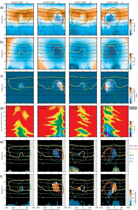
In Fig. 8 we present along-track orbit transects in the 2009 Antarctic early winter. The four columns show a sample of orbit tracks over an 11-day period (day number/orbit num-ber): 2009d136/11, 2009d145/6, 2009d145/13, 2009d147/9. The data in each row are (a) MLS HNO3, (b) T−TICE, (c) temperature history (TTE), (d) temperatures following the Lagrangian back-trajectories, (e) L2PSCMask CALIOP PSC classification, and (f) the post-processed Liquid/Solid index, LS_index=(L−S)/(L+S), whereLis the number of ob-servations in theSTSclassification andSis any other PSC (solid) detection. TheLS_indexis the ratio of the number of CALIOP classifications occurring within the correspond-ing MLS along-track extent, with the extreme values of−1 indicating only solid class and+1 only liquid class detec-tions. TheLS_indexrepresents the dominant PSC classi-fication in a sample volume similar in size to the MLS gas species resolution. The pixel size is much larger than that in the L2PSCMask composition plot, and the composition speckle can be seen as “blocky” regions in theLS_index.

Several contour lines are superposed on the orbit transects: the black–white quasi-horizontal labeled contours show a sample of the MLS pressure levels (HNO3 is retrieved at a six-level/decade change in pressure). The green and blue contours represent temperatures corresponding to theTNAT threshold (using GEOS-5 and MLS HNO3, H2O) andTICE+ 2 K, respectively. The blue temperature contour encompasses an expected HNO3uptake of about 50 % from the gas phase into STS (see Fig. 4a). The yellow contour is the HNO3 12 ppbv contour, and the red contour encloses the area with TTE≥3 days.

Figure 8.Co-located MLS and CALIOP orbit transects for selected orbits showing in six rows:(a)MLS HNO₃.(b)Ambient temperature,

T −TICE.(c)Temperature threshold exposure, TTE (days). (d) Fifteen-day reverse trajectory temperature history,T−TICE, ending at

the 31 hPa pressure level. Minimum temperature encountered along the trajectory is inset at the top left. (e)CALIOP L2PSCMask PSC classification.(f)LS_index. MLS pressure levels are shown as labeled black or white contours. Blue (green) contours indicateTICE+2 K

(TNAT). Red contours indicate TTE values≥3 days. The MLS 12 ppbv HNO3contours are indicated in yellow. Gray shading in(e, f)

Case 2: 25 May 2009/2009d145/6: MLS HNO3shows a substantial region of HNO3uptake over 1500 km and sug-gests a combination of uptake in two separate regions, one located centrally within the local temperature minimum (blue contour,TICE+2 K) and another offset extending to the right edge of the TNAT contour (green). The temperature history (red contour) is the key to this rather apparent asymme-try of the HNO3 distribution with respect to theTNAT con-tour, since the TTE clearly has larger values outside of the central local temperature minimum and is associated with the region of HNO3 uptake on the right. The L2PSCMask (Fig. 8e) shows a substantialSTScloud with some composi-tion speckle, mainly coincident with the central local temper-ature minimum. TheLS_index(Fig. 8f) shows predomi-nantly liquid detections, with more solid detections at the top and lower-right edge of the cloud. TheSTSclass (Fig. 8e) does not completely fill the local temperature contour on the right-hand side, which overlaps with the largest TTE values (red contour).

Case 3: 25 May 2009/2009d145/13: MLS HNO3 shows significant uptake coincident with the peak temperature ex-posure history. The L2PSCMask (Fig. 8e) shows some MIX1/MIX2 class, but is not coincident with the largest HNO3uptake. A very small area of local temperature mini-mum (blue contour), near the along-track distance coordinate at−1000 km and on the 32 hPa level, shows little HNO3 up-take and someSTSclass pixels.

Case 4: 27 May 2009/2009d147/9: MLS HNO3indicates substantial HNO3uptake (Fig. 8a) coincident with the local temperature minimum (blue contour), but also extending to the left edge of theTNATregion (green contour). The greatest exposure to low temperatures (red contour) is associated with the left region of HNO3uptake. The L2PSCMask (Fig. 8e) shows a substantialSTSclass (with multi-class speckle), but only in the right half of the minimum local temperature re-gion. The left half is the area with the largest TTE values (red contour). The L2PSC_Mask showsMIX1/MIX2class pixels below and to the left of the largeSTScloud and also in the regions outside of the TTE andTNATcontours. We also note that although the minimum temperatures along a number of the back trajectories passed below the frost point within 2 days of the MLS/CALIOP observations, no ice PSCs were detected.

Examination of the overlaps between the high TTE val-ues (red contour) and local temperature minima (blue con-tour) in the cases discussed above reveals a correspondence to HNO3uptake but a frequent lack of coincident PSC detec-tions. The local temperatures are just as low (and sufficient for STS formation) as in the areas outside the overlaps, but the STSclass is not seen at all, whereas the TTE increases substantially. The corresponding detailed time histories of the temperatures at 32 hPa are shown in Fig. 8d and reveal that the remarkable asymmetries in the along-track location of HNO3uptake with respect to the local temperature mini-mum distribution can be understood in terms of the different

Figure 9.Comparison of along-track data for a partial orbit on 27 May 2009: (a) MLS HNO3 showing sequestration and the

central region of total denitrification. (b) CALIOP PSC Mask does not show a corresponding large-scale detection of MIX1 clouds.(c)Smoothed CALIOP total backscatter ratio.(d)Smoothed CALIOP perpendicular backscatter ratio. Solid thick white contours are the MLS HNO₃isolines for 7 and 12 ppbv HNO₃. Red contours indicate TTE values≥3 days. The detection of solid particle PSCs is evident in the smoothed CALIOP perpendicular backscatter ratio and extends below the TTE contour by 2–4 km.

density clouds (sedimenting, sub-visibleMIX1) that contain enough condensed HNO3to be detectable through MLS gas-phase depletion, but have low lidar backscatter and are in-visible to CALIOP. Alternatively, it could be argued that the NAT particles grew so large further upstream that they were effectively removed to lower altitudes through sedimentation at the time of the orbit crossing observations, leaving behind a permanently denitrified air mass detected by MLS but with-out coincident CALIOP PSC detections. However, further averaging of CALIOP backscatter (as discussed in Sect. 3) on 27 May, shown in Fig. 9, does indicate a considerably larger area of solid particle detections (MIX1class), associ-ated with the high TTE region, and so it appears that we are dealing with the limit of the L2PSCMask detection range. Sedimentation of large NAT is suggested by the 2–4 km re-gion of solid particle detections lying below the high TTE region.

4.2 Denitrification and renitrification

The Antarctic gas-phase HNO3distribution shown in Fig. 10 provides a record of the effects of the formation and dissipa-tion of PSCs and is displayed as the daily areal coverage for equivalent latitudes less than 60◦S, for isentropic levels from 340 to 500 K. The white solid lines indicate low, median, and high values of the HNO3 probability density function. The minimum HNO3 mixing ratios (i.e., the colored region be-low the 10th percentile white line) indicate that PSCs can lead to a complete removal of the available ambient HNO3 from the gas phase. As shown in Lambert et al. (2012), the spread of HNO3 mixing ratios in totally denitrified regions is compatible with the MLS precision. The temperature de-crease starts from the upper levels of the vortex and descends over time, resulting in PSCs and HNO3 uptake developing later at the lower levels. The maximum HNO3mixing ratios (i.e., the colored region above the 90th percentile white line) indicate episodes of renitrification at the lower levels aris-ing from the sedimentation of PSCs. As the NAT particles fall through lower levels, they may pass into regions where they are less thermodynamically stable. In these cases the evaporative release of HNO3from the condensed phase in-creases the gas-phase values, and this is detected as a rise in the HNO3 measured by MLS at the lower levels. The pro-cess is seen quite clearly in the increasing time lag between the appearance of anomalously large HNO3values above the 90th percentile at 420 K May) compared to 340 K (mid-June). This process acts to raise the NAT temperature exis-tence threshold at the lower levels because of the enhanced gas-phase HNO3and therefore increases the likelihood of oc-currence of NAT. Heterogeneous chemical reactions on the PSC particles involving ClONO2 and N2O5 produce addi-tional HNO3, which remains in the condensed phase until the PSC dissipates (Turco et al., 1989). Therefore, an in-crease in gas-phase HNO3at a given level may arise from the evaporation either of sedimenting PSCs from above or

Figure 10.Time series of the distribution of MLS HNO3 in the

Antarctic from May to October 2009, for equivalent latitudes less than 60◦S, and for isentropic levels from 340 to 500 K. Major tick marks indicate the beginning of the month. The color scale indicates the areal coverage. White solid lines indicate the 10th, 20th, 50th (i.e., median), 80th, and 90th percentiles of the HNO3probability

density function.

Figure 11.Twenty-day time series of Antarctic raster plots at 68, 46, 32, and 21 hPa in 2009 from day number 132 (12 May) to 151 (31 May). Gray shading indicates no observations; olive-green shading indicates observations but no detections.(a)MLS HNO3. Numbers on the right

axis indicate the median HNO₃for the region where TTE>2 days (in ppbv) for each day at 32 hPa.(b)Temperature history. A set of three numbers on the right axis for each day at 32 hPa indicates in ascending order (i) maximum TTE in days, (ii) minimum local temperature,

T−TICEin K, (iii) minimum temperature encountered along the back-trajectory, andT−TICEin K.(c)CALIOPLS_index.(d)CALIOP

PSC fraction. Numbers on the right axis indicate the maximum PSC fraction (ratio of the number of PSC detections to the number of observations) for each day at 32 hPa.

5 Time series of PSC formation and Lagrangian temperature history

In this section we examine the formation of PSCs and the La-grangian temperature history during the early 2009 Antarc-tic PSC season. Figure 11 shows a time series of data taken over the 20 days from 2009d132 to 2009d151 (12–31 May) of HNO3, TTE (temperature history),LS_index, and PSC fraction. Averaging bins are as described in Sect. 4.1. There are four columns in each panel corresponding to four pres-sure levels at 68, 46, 32, and 21 hPa. Each “mini-plot” (e.g., identified by HNO32009d132 68 hPa) is a raster image with

fraction is the ratio of the number of PSC detections to the total number of observations in each averaging bin.

Significant TTE first appears on the 32 hPa level close to the South Pole on 2009d134/2009d135 (14–15 May), gradu-ally increases in area, and expands in vertical extent rapidly to the 46 hPa level and eventually to the 68 and 21 hPa levels with a delay of about a week. Note the lack of corresponding areal coverage of PSCs, especially on the 32 hPa level (only a few PSC detections are scattered about; see the PSC fraction panel). The PSCLS_indexindicates some predominantly solid class PSC detections at 68 and 46 hPa before 2009d141 (21 May), but there are fewer detections at 32 hPa. However, MLS indicates HNO3uptake on the 32 hPa level starting ear-lier from 2009d135 (15 May) that is as widespread as that on the 46 hPa level and similar in areal extent to the TTE. At 68 hPa there is evidence for an increase in HNO3 fol-lowing 2009d139 (19 May), presumably due to renitrifica-tion from evaporating NAT PSCs that have sedimented from a higher level. The combined data at 32 hPa indicate that, in the early period, the CALIOP L2PSCMask is not detecting PSCs, since there is a persistent area of daily HNO3depletion that is not matched by corresponding PSC detections but is consistent with the temperature history. We use the term sub-visible PSCs to refer to these cases (i.e., significant depletion of gas-phase HNO3, but without detection by CALIOP).

We examine the variation of MLS HNO3 with TTE for sub-visible PSCs in the period 2009d135–2009d144 (15– 24 May) in more detail in Fig. 12. The scatter plot of the gas-phase HNO3 values shows a range of ∼4 ppbv (from ∼14 to∼18 ppbv) for low TTE, and as TTE increases be-yond∼1 day, the HNO3decreases. A highly simplified mi-crophysical model has been used to calculate the uptake of HNO3from the gas phase. Growth of NAT by vapor depo-sition has been calculated in the manner outlined by Toon et al. (1989) and following the simplifications introduced by Carslaw et al. (2002). Here, we ignore sedimentation and cal-culate the growth of monodisperse NAT in a constant temper-ature atmosphere (TICE+4 K) for two different initial NAT densities (5×10−4 and 5×10−5cm−3) and two initial to-tal HNO3values that encompass the observed range (14 and 18 ppbv). The NAT growth model is initialized with a 0.1 µm radius at the nucleation time (TTE=0), and the subsequent time evolution of the gas-phase HNO3is plotted as colored curves indicating the NAT particle radius. These two curves practically bound the MLS observations of the distribution of gas-phase HNO3as a function of TTE. As is well known, low NAT number densities produce large NAT particles (Jensen et al., 2002), which take several days to reach thermodynamic equilibrium (the uptake curves bottom out after 15 days or more). Backscatter calculations for NAT with characteris-tics of the upper curve (assuming ǫ=0.9) show that the backscatter (perpendicular or total) is below the CALIOP threshold of detection along the entire time evolution. For the lower curve, the higher NAT number density limits the particle growth to a much smaller radius, and backscatter

Figure 12.MLS HNO3on the 32 hPa pressure level over the 10-day

period from 15 to 24 May 2009 (days 135–144) in the Antarctic po-lar vortex. Data are selected only if there are no coincident PSC detections by CALIOP.(a)Scatter plot of individual HNO3values

vs. TTE. The colored dots indicate the measurement day number (given in the inset color bar). The two colored curves are from a calculation of the gas-phase HNO₃, assuming growth of NAT at a constant temperature ofTICE+4 K for NAT number densities and

initial total HNO₃values of 5×10−5cm−3 and 18 ppbv, respec-tively, for the upper curve and 5×10−4cm−3and 14 ppbv for the lower curve. The top color bar indicates the NAT radius.(b)As in (a)except plotted as a 2-D histogram of the density of points, with the inset color bar giving the number of samples per bin. Only bins accumulating two or more data points are shown.

Figure 13.Thirty-day time series of Antarctic raster plots at 32 hPa for 2006–2015. Diamond symbols indicate the last day before the start of detectable HNO₃depletion. Gray shading indicates no observations; olive-green shading indicates observations but no detections. Day number is shown on the vertical axis.(a)MLS gas-phase HNO3.(b)CALIOPLS_index.

can be accounted for qualitatively by a NAT population char-acterized by low number densities/large radii.

6 Interannual variations in the early Antarctic PSC season

In this section we investigate the interannual variability of Antarctic PSCs and HNO3 over the past decade and again make use of the geolocated raster plot format discussed in Sect. 2.4. Figure 13 shows the MLS HNO3 and CALIOP LS_indexat 32 hPa for 30 days from day number 132 to 161 (12 May to 10 June) for the years 2006–2015. The cor-responding time series for TTE and T−TICE are shown in Fig. 14. Additionally, in Fig. 15, we present a complemen-tary side-by-side comparison of the same observations by plotting the MLS HNO3as a time series with each

Figure 14.Thirty-day time series of Antarctic raster plots at 32 hPa for 2006–2015. Day number is shown on the vertical axis.(a)TTE (days).(b)T−T_ICE(K).

pool temperatures and the polar vortex are highly concentric. We have also investigated the daily scatter of temperature vs. vorticity in the ERA-Interim reanalysis data (not shown here), and find that the annular region 60 to 82◦S (visible to Aura and CALIOP) describes adequately the state of the region poleward of 82◦S (not sampled by Aura or CALIOP). The start of the PSC season appears to display two modes (see Figs. 13b and 15b), with some years having larger cover-age of solid PSCs (2007, 2011, and 2014) than others, which show larger coverage of liquid PSCs (2008, 2009, 2010, and 2015). We identify the presence of sub-visible PSCs by a delay between the onset of gas-phase HNO3depletion (see Figs. 13a and 15a) and the geophysically associated detec-tion of PSCs (see Figs. 13b and 15b). Table 2 lists the day number of the initial onset of HNO3depletion, the first day of detection of PSCs by CALIOP, the presence of sub-visible PSCs, and the predominant PSC class (solid or liquid) for the first few days following detection. Sub-visible clouds

Table 2.Comparison of times of occurrence of HNO3depletion and detection of PSCs at the start of each PSC season.

Year Onset day of HNO3depletion First day of PSC detection Sub-visible PSCs Dominant PSC class

2006 148 ∗ ∗ ∗

2007 137 137 No SOL

2008 145 147 Yes LIQ

2009 135 141 Yes LIQ

2010 140 141 Yes LIQ

2011 140 141 Yes SOL

2012 139 ∗ ∗ ∗

2013 138 ∗ ∗ ∗

2014 133 139 Yes SOL

2015 139 139 No LIQ

∗_{indicates no MLS and CALIOP overlap.}

Höpfner et al. (2009) and Spang et al. (2016) presented in-tercomparisons of CALIOP vs. MIPAS PSC detections and statistics on the frequency of type classifications that are rele-vant here. During May, considerably more MIPAS-only PSC detections (i.e., without corresponding matching detections by CALIOP) were found by Höpfner et al. (2009), and even with longer-term averaging, over the entire May–October pe-riod, Spang et al. (2016) concluded that MIPAS has higher sensitivity to PSCs since, for the cases where CALIOP de-tects no cloud, about 60 % correspond to cloudy scenes for MIPAS. Therefore, these MIPAS/CALIOP comparisons sup-port our conclusion that CALIOP is not sensitive to low num-ber density and large particle NAT.

The goal of describing the interannual variability of PSC seasons within the context of a decadal climatology can be met by synthesizing the CALIOP and MLS observations, consisting of the four-variable dataset (HNO3, TTE,T−TICE andLS_index), into a number of characteristic groups or clusters and thereby capturing the major characteristics of PSC formation. Simple partitioning obtained by setting a sin-gle threshold boundary on each of the four variables would result in 16 different PSC groups (some of which may be empty). Such a large number of groupings would complicate interpretation, and so a more parsimonious scheme is desir-able to enforce a reduction in the number of groups. Cluster analysis (CA) is a well-established tool for unsupervised ex-ploration of a dataset (Jain, 2010). Ideally members of the same cluster (identified by their proximity to the cluster cen-troid) will naturally exhibit similar intrinsic properties and display low within-cluster variance, whereas the differences amongst the members of one cluster to another will display high between-cluster variance. We used aKmeans centroid algorithm with a Euclidian distance metric to partition the four-variable dataset after performing zero mean and unit variance normalization. K means analyses were performed for a varying number of imposed clusters (K=2 toK=20), and the gap statistic (Tibshirani et al., 2001) was used to as-sess the optimal number of clusters by comparison with

uni-formly random data and an uncorrelated dataset obtained by randomly reordering the measurement times of the four vari-ables. A steep rise in the gap statistic was observed over the rangeK=2 toK=7, followed by a flattened plateau re-gion out to K=20 (not shown). The clusterings obtained forK=6 are shown in Table 3 and Fig. 16 for all the years 2006–2015. TheK=6 case was chosen because the clus-ters fell practically into two sets (a, b) of three groups, corre-sponding to predominantly liquid (Fig. 16a,LS_index>0) and predominantly solid (Fig. 16b,LS_index<0) PSCs. No particular improvement was observed for theK=7 case. TheLS_index vs. day number scatter plot indicates that there is some cross-over of liquid/solid PSCs present in both the a1 and a2 groups. The groups are presented superposed as a scatter plot on the thermodynamic HNO3vs.T−TICE di-agram and show clearly that the two sets (a, b) are associated with the STS and NAT equilibrium branches. As in previ-ous analyses, the NAT population exhibits considerable non-equilibrium effects (Lambert et al., 2012; Pitts et al., 2013), with the temperature distribution extending to temperatures as low as the STS branch. No correction has been made for the suspected temperature bias in the meteorological temper-ature data (Sect. 3.2).

Figure 15.Time series for the Antarctic for associated HNO3and PSCs during 2006–2015 at 32 hPa.(a)MLS HNO3vs. day number. The

color scale shows the TTE. Only data for TTE>0.1 day are plotted. The inset pie charts indicate the relative proportions of measurements in six categories (red–yellow sectors are solid PSCs; purple–blue sectors are liquid PSCs) as defined in the text and in Fig. 16.(b)CALIOP LS_indexvs. day number. The color scale shows theLS_index. Gray shading indicates no measurements. Light green shading in (b)indicates the envelope of MLS HNO3observations in(a).

are advected downstream (Lambert et al., 2012) away from their gravity-wave sites of origin.

Compelling evidence of the differences in the formation of liquid and solid PSCs can be deduced from comparisons of the temperature history of the groups. For the case of moder-ate gas-phase HNO3depletion, the occurrence of liquid PSCs (a3) shows a steep fall-off in the TTE distribution beyond

conse-Figure 16.Results of theK=6 cluster analysis of the combined MLS and CALIOP data for the Antarctic for the years 2006–2015 at 32 hPa. Thermodynamic diagrams indicate for reference the theoretical HNO3uptake by STS (blue–black dashed line) and by NAT (green–black

dashed line). The scatter plots show the MLS HNO₃vs. temperature relative to the ice frost point colored by the correspondingLS_index obtained from CALIOP. Columna(b) shows the data in three groupsa1–a3(b1–b3), which are seen to be predominantly liquid (solid) PSC detections according to theLS_index. The colored contours (a1– purple,a2– dark blue,a3– light blue,b1– red,b2– orange,b3 – yellow) contain 95 % of the corresponding cluster members. The maps show the geographic distribution of the members of each of the clusters and are color-coded by theLS_index(inset color bar). A 2-D view (HNO3vs. TTE) is provided of the cluster densities (purple–

yellow shading indicates low to high density) and the accompanying colored solid lines represent the normalized 1-D histogram of the TTE values. The cluster densities are also displayed as a 2-D view ofLS_indexvs. day number.

Table 3.Results of theK=6 cluster analysis for 2006–2015: the number of members assigned to each group, the mean and standard deviation of the relative number of observations, and the centroids in the four-variable data space are given.

Group LIQ/SOL Number Mean Standard HNO3 TTE T−TICE LS_index

name (%) deviation (%) (ppbv) (days) (K)

a1 LIQ 3194 14 8 1.41 11.22 0.07 0.56

a2 LIQ 5139 23 7 2.84 3.30 0.67 0.55

a3 LIQ 3532 18 9 11.19 0.88 3.10 0.60

b1 SOL 3194 16 10 1.33 6.80 0.71 −0.73

b2 SOL 4206 24 10 9.04 1.61 4.00 −0.83