Sensitivity of ensemble Lagrangian reconstructions to assimilated wind time step resolution

(1)

ACPD

9, 8619–8633, 2009

Sensitivity of Lagrangian reconstructions to

wind resolution

I. Pisso et al.

Title Page

Abstract Introduction

Conclusions References

Tables Figures

◭ ◮

Back Close

Full Screen / Esc

Printer-friendly Version

Interactive Discussion

Atmos. Chem. Phys. Discuss., 9, 8619–8633, 2009 www.atmos-chem-phys-discuss.net/9/8619/2009/ © Author(s) 2009. This work is distributed under the Creative Commons Attribution 3.0 License.

Atmospheric Chemistry and Physics Discussions

This discussion paper is/has been under review for the journalAtmospheric Chemistry and Physics (ACP). Please refer to the corresponding final paper inACPif available.

Sensitivity of ensemble Lagrangian

reconstructions to assimilated wind time

step resolution

I. Pisso1,*, V. Mar ´ecal2, B. Legras1, and G. Berthet2

1

Laboratoire de M ´et ´eorologie Dynamique (UMR 8539), ENS – CNRS, Paris, France 2

Laboratoire de Physique et Chimie de l’Environnement et de l’Espace (UMR 6115), Universit é d’Orl éans – CNRS, Orl éans, France

*

now at: Department of Applied Mathematics and Theoretical Physics, University of Cambridge, Cambridge, UK

Received: 20 January 2009 – Accepted: 25 February 2009 – Published: 1 April 2009

Correspondence to: I. Pisso ([email protected])

(2)

ACPD

9, 8619–8633, 2009

wind resolution

I. Pisso et al.

Title Page

Tables Figures

◭ ◮

Back Close

Full Screen / Esc

Abstract

The aim of this study is to define the optimal temporal and spatial resolution required for accurate offline diffusive Lagrangian reconstructions of high resolution in-situ tracers measurements based on meteorological wind fields and on coarse resolution 3-D tracer distributions. Increasing the time resolution of the advecting winds from three to one 5

hour intervals has a modest impact on diffusive reconstructions in the case studied. This result is discussed in terms of the effect on the geometry of transported clouds of points in order to set out a method to assess the effect of meteorological flow on the transport of atmospheric tracers.

1 Introduction

10

The calculation of Lagrangian backward trajectories has become a widely accepted technique. Applications range from chemical modelling to environmental and nuclear risk management. Since the seminal work of Sutton (1994) and Norton (1994) the tools and the advecting fields have been steadily improving.

Chemical tracer distributions can be reconstructed based on 3-D tracer fields and 15

trajectories. Parcel trajectories are known to be extremely sensitive to the advecting wind due to the chaotic nature of the atmosphere.

This effect is controlled by adding (vertical) stochastic diffusion to ensembles of tra-jectories (Legras et al., 2005; Pisso and Legras, 2008) based on Green’s function prop-erties which significantly improve the quality of tracer reconstructions. The choice of 20

temporal and spatial resolution of wind fields used to calculate trajectories is a major problem. It has been shown that the standard 6-hourly sampled winds may produce large overestimates of the tracer concentration fluctuations (Legras et al., 2005).

The combined use of analyses and forecasts allows one to obtain 3-hourly sampled wind-fields (Stohl et al., 2005; Bregman et al., 2006) which provide more accurate 25

(3)

ACPD

9, 8619–8633, 2009

wind resolution

I. Pisso et al.

Title Page

Tables Figures

◭ ◮

Back Close

Full Screen / Esc

question arises whether further improvement can be obtained at higher resolutions. The goal of this work is to investigate, for a case study, the optimal temporal and spa-tial resolution of advecting winds needed to perform Lagrangian tracer reconstructions. To achieve this, we measure the effect of changing time and space resolution on the reconstruction of observations based on our previous study (Pisso and Legras, 2008) 5

which used ensembles of diffusive backward trajectories. The selected tropical O3

pro-file presents an interesting feature associated with an extratropical intrusion used to benchmark di_fferent model setups.

The back trajectories are initialized using the ozone 3-D outputs from the REPROBUS Chemistry-Transport Model (Lef `evre et al., 1998) as done in previous 10

studies. Trajectories are calculated using operational ECMWF wind fields with time resolutions of 6, 3, and 1 h. To our knowledge, this work had never been undertaken before since no operational center provides forecast fields with a temporal resolution shorter than 3 h. Therefore special forecast experiments were carried out to get hourly fields.

15

2 Data and methods

2.1 Tracer data

The ozone profile (Fig. 1) was collected by the Solid State Ozone Sensor instrument (Hansford et al., 2005) during the Hibiscus campaign (Pommereau et al., 2007) over Bauru, Brazil (49.0 W, 22.4 S) on 13 February 2004. The sampling frequency is about 20

1 Hz, yielding more than 10 000 measurement points. The ozone peak observed

(4)

ACPD

9, 8619–8633, 2009

wind resolution

I. Pisso et al.

Title Page

Tables Figures

◭ ◮

Back Close

Full Screen / Esc

2.2 Back trajectories

Diffusive back trajectories are calculated with TRACZILLA (Legras et al., 2003, 2005; Pisso and Legras, 2008), a modified version of FLEXPART (Stohl et al., 2005) which uses a direct vertical interpolation of ECMWF winds, from hybrid levels, with a time step of 900 s. Different diffusive reconstructions of the Hibiscus O3 profile are performed

5

using different time/spatial resolutions.

A special experiment using the version of ECMWF model (CY28R1) operational at the time of the observations is employed. The first 12-h forecast fields are archived every hour instead of the standard 3-hourly time interval. The 12-h short term forecasts start from the analysis at 00:00 UTC and 12:00 UTC. The version of the ECMWF model 10

used has a T511 spectral truncation corresponding to a horizontal resolution of the order of 60 km with 60 vertical levels.

The reconstructions based on 6-hourly winds use the ECMWF standard operational analyses at 00:00 UT, 06:00 UT, 12:00 UT and 18:00 UT interpolated on a 1◦×1◦ grid. Those based on 3-hourly winds use the same analyses and at the intermediate times 15

the 3-h and 9-h forecasts started from the 00:00 UT and 12:00 UT analyses interpolated on a 1◦×1◦ grid. The last set of reconstructions based on hourly winds extends the 3-hourly experiment by using the specially archived hourly forecasts described above. For the hourly winds, in addition to the experiments with 1◦×1◦and to be consistent with the finer time resolution, we refine the spatial resolution interpolating the wind fields on 20

a horizontal 0.5◦×0.5◦ grid. In all the cases the vertical resolution is the original one (60 levels).

Three values of diffusivity (D) (0.1 m2s−1, 0.5 m2s−1, 1 m2s−1) were used to recon-struct the measured profile for the temporal and spatial resolution of each wind field. This experimental design is based on the study by Pisso and Legras (2008) who inves-25

(5)

ACPD

9, 8619–8633, 2009

wind resolution

I. Pisso et al.

Title Page

Tables Figures

◭ ◮

Back Close

Full Screen / Esc

only.

2.3 3-D chemical fields

Chemical mixing ratios are interpolated from REPROBUS three-dimensional (3-D) out-put fields. REPROBUS (REactive Processes Ruling the Ozone BUdget in the Strato-sphere) is a 3-D chemical-transport model with a comprehensive treatment of gas 5

phase and heterogeneous chemical processes in the stratosphere (Lef `evre et al., 1998). Long-lived species, including ozone, undergo advection by a semi-Lagrangian scheme forced by 3-hourly ECMWF meteorological data constructed from analyses and forecasts instead of using common 6-hourly analysis.

The model is integrated on 42 hybrid pressure levels that extend from the ground up 10

to 0.1 hPa, with a horizontal resolution of 2◦ latitude by 2◦ longitude. The simulation was initiated on 1 April 2002 using the 3-D ECMWF analysis for ozone and an April zonal mean computed from a long-term simulation of REPROBUS for other species.

3 Results

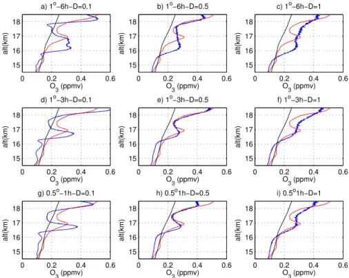
The di_ffusive reconstructions displayed in Fig. 1 present fine scale structures which 15

are absent from the REPROBUS dataset interpolated at the time and location of the measurements. This illustrates how spatial information about the fine scale structure can be extracted by the reconstruction method from the initial chemical field and a time series of wind fields, both at coarser resolution. This is seen more clearly with small values of diffusivity (D₌0.1 m2s−1) because high values tend to smooth the small-20

(6)

ACPD

9, 8619–8633, 2009

wind resolution

I. Pisso et al.

Title Page

Tables Figures

◭ ◮

Back Close

Full Screen / Esc

Lagrangian CTMs. ForD₌0.1 m2s−1(panel a) the 6 hourly reconstruction exhibits spu-rious small fluctuations and the ozone peak is shifted downwards by almost 1000 m. For D₌0.5 m2s−1(panel b) and D₌1 m2s−1(panel c) the fluctuations disappear be-cause of the increase of diffusivity but the peak remains shifted with respect to the measurements.

5

For the 3-hourly reconstructions (second row in Fig. 1), results with

D₌0.1 m2s−1(panel d) show less agreement with the measurements than with

D₌0.5 m2s−1(panel e) but in both cases the shift is reduced down of about 200 m. The valueD₌1 m2s−1(third column) is too high to give detailed small scale structures. Nevertheless, the 3-hourly reconstruction (panel f) is more accurate than the 6-hourly 10

one (panel c). The comparison between the second and the third rows in Fig. 1 shows small di_fferences between reconstructions carried out with a 3-hourly temporal resolu-tion and a 1◦×1◦ spatial resolution than those with a hourly temporal resolution and a 0.5◦×0.5◦spatial resolution.

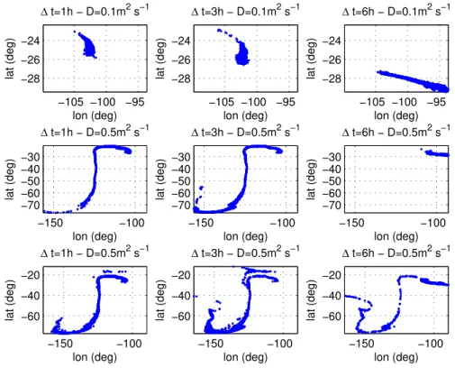
To explain the small differences obtained between the hourly and the 3-hourly recon-15

structions, we use the locations of the trajectory points att₌−192 h (the backward time used for the reconstructions) before the measurements to analyse the influence of the resolution on the advective transport. Figure 2 displays, att₌₋192 h, the locations of a cloud of points advected backwards using different values ofDand∆t(time step for the advecting winds). This ensemble of points is chosen because it corresponds to the 20

most interesting feature of the measured profile, the ozone peak at 17 km altitude. Fig-ure 2, first row (D₌0.1 m2s−1), clearly shows that the clouds of points for the 1-hourly and 3-hourly reconstructions are close and largely overlap while they are disjoint from the cloud of points provided by the 6-hourly reconstruction. In Fig. 2 the cloud of points provided by the 6-hourly reconstructions is close to the eastern part of the cloud of 25

points provided by the 1-hourly and 3-hourly reconstructions. ForD₌1 m2s−1the dif-ferences tend to be smaller, because the competing diffusion hinders the effect of the global perturbation in the wind field.

(7)

ACPD

9, 8619–8633, 2009

wind resolution

I. Pisso et al.

Title Page

Tables Figures

◭ ◮

Back Close

Full Screen / Esc

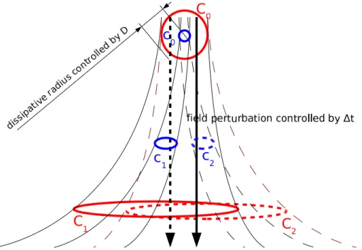
flow associated with the time series of wind fields. The schematic in Fig. 3 illustrates the relationship between sensitivity to initial conditions and turbulent di_ffusion. Consider a point lying on either side of a separatrix associated with the stable manifold of an hyperbolic point which is displaced by the global perturbation of the advecting field. A neighborhood of this point (associated with an in situ measurement) corresponds to 5

a cloud of points, whose “dissipative radius” (the radius of the cloud after the initial stage dominated by diffusion, Legras et al., 2005) depends on the stochastic noise related to the di_ffusivity coe_fficientD. The final (backwards in time here) distribution of an advected cloud (c₀) may change in the perturbed (c₁) and unperturbed case (c₂) (on either side of the separatrix) if the initial radius is smaller than the displacement 10

of the separatrix. In which case, the cloud of points (c₀) visits di_fferent locations and samples different air masses. On the other hand, if the initial radius is large (C₀) with respect to the displacement of the separatrix, the supports of the clouds advected by the original and the perturbed flows will overlap and, as time increases, the di_fference tends to zero. The schematic in Fig. 3 points out why for large enough values of D

15

the change in wind resolution has a reduced effect, whereas for small diffusivity the change in resolution may be significant. The effect on the reconstructions will be large if the deviation of the flow due to increased resolution exceeds the diffusive radius or the resolution of the chemical initialization field.

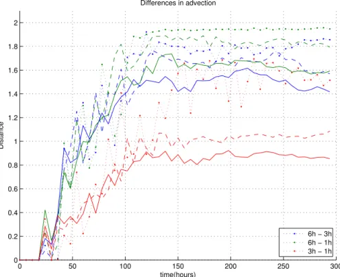
To make an objective comparison between the positions associated with different re-20

constructions, we have calculated the distance between the convex hull of two clouds taking into account the particle density. The distance between two clouds is defined as dist (C₁, C₂;t)=R|f(C₁;t)−f(C₂;t)|dx wheref(C;t) is the probability distribution in space of the cloudC at time t. A histogram of the trajectory positions within a CTM grid is used to estimatef(.;.). The function dist (., .;.) is a distance over the classes 25

(8)

ACPD

9, 8619–8633, 2009

wind resolution

I. Pisso et al.

Title Page

Tables Figures

◭ ◮

Back Close

Full Screen / Esc

is smaller than between 1-hourly and 6-hourly and between 3-hourly and 6-hourly re-constructions. This suggests that the hourly and 3-hourly wind fields provide similar trajectories and therefore similar dynamical fields which are both different from the 6-hourly wind fields. Both Figs. 2 and 4 show large differences between the location of the clouds of points for the same time/spatial resolution but different diffusivity val-5

ues. Using 3-hourly and 1-hourly wind fields, the trajectories forD₌0.1 m2s−1mainly come from the subtropics 192 h before the measurements while they originate from a large range of latitudes from the subtropics to the polar regions forD₌0.5 m2s−1. This means that the diffusivity is a key parameter in the reconstruction methods significantly affecting the location of the trajectories. This is consistent with the results in Fig. 1 10

showing larger differences in the reconstructed profiles when varying D values than when using 1-hourly instead of 3-hourly time resolution.

Consequently, our results suggest that whenDis 0.5 m2s−1increasing the time res-olution from 3 to 1 h does not significantly modify the trajectory of the tracer recon-structions. The differences in the tracer flow produced by wind using different time step 15

resolutions can be assessed numerically (Demazure, 2000). In this study we have quantified the effect of such perturbation to establish comparison with high resolution in situ experimental measurements.

4 Conclusions

We have studied the influence of temporal and spatial resolution on advective transport 20

on tracer profile Lagrangian reconstructions. We have focused on one case study in the subtropics in February 2004, comparing very high resolution O3in-situ measurements

with Diffusive Ensemble Reconstructions calculated using as advecting winds standard meteorological analysis (6 h time step), with interim hourly and 3-hourly forecasts cal-culated with the ECMWF model. The use of hourly fields instead of 3-hourly fields does 25

(9)

ACPD

9, 8619–8633, 2009

wind resolution

I. Pisso et al.

Title Page

Tables Figures

◭ ◮

Back Close

Full Screen / Esc

for the reconstruction. Although the results obtained on this case study are limited to the time and location of the measurements used to calculate the reconstructions, they support the use of a 3-hourly time resolution and a 1◦×1◦spatial resolution. One could argue that the reconstructions done in this study are limited by the REPROBUS output fields having a coarse 2◦×2◦resolution. However, previous studies (Legras et al., 2005) 5

suggest that the coarse resolution of initial tracer fields does not play a major role. The results presented here also show that using hourly wind fields in the reconstructions does not add significant information on the atmospheric dynamics. This suggests that in the ECMWF analyses and 12 h forecasts for 2004 the information contained at the scale of 1 h/0.5◦×0.5◦ is not significantly different from the information contained at 10

3 h/1◦×1◦. This might not apply to more recent versions of the analysis performed at higher resolution but can be taken as valid also for analyses or reanalysis performed at a lower resolution.

This study sets out a technique to assess the optimal space and time resolutions for ensemble Lagrangian reconstructions in the lower stratosphere. The robustness 15

of the reconstructions is associated with the structural stability of atmospheric flows under perturbations (Demazure, 2000) like those introduced by changes in resolution and parametrization tunings. The local tools and results presented in the present study can be extended to the global scale to study the movement of tracers. However, the question of the optimal temporal/spatial resolution for off-line calculations is certainly 20

model-dependent and in practice unsolved.

Acknowledgements. We acknowledge the Hibiscus team for O₃ data and Franck Lef `evre for support on the Reprobus model. I. Pisso was funded with a fellowship of the Ecole Poly-technique. This work was funded by the European Union SCOUT-O3 Project (GOCE-CT-2004505390).

(10)

ACPD

9, 8619–8633, 2009

wind resolution

I. Pisso et al.

Title Page

Tables Figures

◭ ◮

Back Close

Full Screen / Esc

The publication of this article is financed by CNRS-INSU.

References

Berthet, G., Huret, N., Lef ´evre, F., Moreau, G., Robert, C., Chartier, M., Catoire, V., Barret, B., Pisso, I., and Pomathiod, L.: On the ability of chemical transport models to simulate the 5

vertical structure of the N₂O, NO₂and HNO₃species in the mid-latitude stratosphere, Atmos.

Chem. Phys., 6, 1599–1609, 2006,

http://www.atmos-chem-phys.net/6/1599/2006/. 8623

Bregman, B., Meijer, E., and Scheele, R.: Key aspects of stratospheric tracer modeling using assimilated winds, Atmos. Chem. Phys., 6, 4529–4543, 2006,

10

http://www.atmos-chem-phys.net/6/4529/2006/. 8620, 8623

M. Demazure: Bifurcations and Catastrophes, Geometry of Solutions to Nonlinear Problems, Universitext, Springer, Berlin, 268 pp., 2000. 8626, 8627

Hansford, G. M., Freshwater, R. A., Bosch, R. A., Anthony Cox, R., Jones, R. L., Pratt, K. F. E., and Williams, D. E.: A low cost instrument based on a solid state sensor for balloon-borne 15

atmosphericO₃profile sounding, J. Environ. Monitor., 7, 158–162, 2005. 8621

Lef `evre, F., Figarol, F., Carslaw, K., and Peter, T.: The 1997 arctic ozone depletion quantified from three-dimensional model simulations, Geophys. Res. Lett., 25, 2425–2428, 1998. 8621, 8623

Legras, B., Joseph, B., and Lef `evre, F.: Vertical diffusivity in the lower stratosphere from

20

Lagrangian back-trajectory reconstructions of ozone profiles, J. Geophys. Res., 108(D18), 4562, doi:10.1029/2002JD003045, 2003. 8622

Legras, B., Pisso, I., Berthet, G., and Lef `evre, F.: Variability of the Lagrangian turbulent diffusion

in the lower stratosphere, Atmos. Chem. Phys., 5, 1605–1622, 2005,

(11)

ACPD

9, 8619–8633, 2009

wind resolution

I. Pisso et al.

Title Page

Tables Figures

◭ ◮

Back Close

Full Screen / Esc

Norton, W. A.: Breaking rossby waves in a model stratosphere diagnosed by a vortex-following coordinate system and a technique for advecting material contours, J. Atmos. Sci., 51, 654– 673, 1994. 8620

Pisso, I. and Legras, B.: Turbulent vertical diffusivity in the sub-tropical stratosphere, Atmos.

Chem. Phys., 8, 697–707, 2008, 5

http://www.atmos-chem-phys.net/8/697/2008/. 8620, 8621, 8622

Pommereau, J.-P., Garnier, A., Held, G., Gomes, A.-M., Goutail, F., Durry, G., Borchi, F., Hauchecorne, A., Montoux, N., Cocquerez, P., Letrenne, G., Vial, F., Hertzog, A., Legras, B., Pisso, I., Pyle, J. A., Harris, N. R. P., Jones, R. L., Robinson, A., Hansford, G., Eden, L., Gardiner, T., Swann, N., Knudsen, B., Larsen, N., Nielsen, J., Christensen, T., Cairo, F., 10

Pirre, M., Mar ´ecal, V., Huret, N., Rivi ´ere, E., Coe, H., Grosvenor, D., Edvarsen, K., Di Don-francesco, G., Ricaud, P., Berthelier, J.-J., Godefroy, M., Seran, E., Longo, K., and Freitas, S.: An overview of the HIBISCUS campaign, Atmos. Chem. Phys. Discuss., 7, 2389–2475, 2007,

http://www.atmos-chem-phys-discuss.net/7/2389/2007/. 8621 15

Stohl, A., Forster, C., Frank, A., Seibert, P., and Wotawa, G.: Technical note: The Lagrangian particle dispersion model FLEXPART version 6.2, Atmos. Chem. Phys., 5, 2461–2474, 2005, http://www.atmos-chem-phys.net/5/2461/2005/. 8620, 8622

Sutton, R.: Lagrangian flow in the middle atmosphere, Q. J. Roy. Meteorol. Soc., 120B(519), 1299–1320, 1994. 8620

(12)

ACPD

9, 8619–8633, 2009

wind resolution

I. Pisso et al.

Title Page Abstract Introduction Conclusions References Tables Figures ◭ ◮ ◭ ◮ Back Close

Full Screen / Esc

0 0.2 0.4 0.6

15 16 17 18

a) 1o−6h−D=0.1

alt(km)

O

3 (ppmv)

0 0.2 0.4 0.6

15 16 17 18

d) 1o−3h−D=0.1

alt(km)

O

3 (ppmv)

0 0.2 0.4 0.6

15 16 17 18

g) 0.5o−1h−D=0.1

alt(km)

O₃ (ppmv)

0 0.2 0.4 0.6

15 16 17 18

b) 1o−6h−D=0.5

alt(km)

O

3 (ppmv)

0 0.2 0.4 0.6

15 16 17 18

e) 1o−3h−D=0.5

alt(km)

O

3 (ppmv)

0 0.2 0.4 0.6

15 16 17 18

h) 0.5o1h−D=0.5

alt(km)

O₃ (ppmv)

0 0.2 0.4 0.6

15 16 17 18

c) 1o−6h−D=1

alt(km)

O

3 (ppmv)

0 0.2 0.4 0.6

15 16 17 18

f) 1o−3h−D=1

alt(km)

O

3 (ppmv)

0 0.2 0.4 0.6

15 16 17 18

i) 0.5o1h−D=1

alt(km)

O₃ (ppmv)

Fig. 1. Red, black and blue lines represent respectively the measured O₃ profile, the profile at the time and location of the measurement interpolated directly from REPROBUS and the

profile provided by a diffusive reconstruction. Each row corresponds to a given temporal and

space resolution and each column to a given diffusivityDvalue. The horizontal axis represents

(13)

ACPD

9, 8619–8633, 2009

wind resolution

I. Pisso et al.

Title Page Abstract Introduction Conclusions References Tables Figures ◭ ◮ ◭ ◮ Back Close

Full Screen / Esc

Interactive Discussion −105 −100 −95

−28 −26 −24

lon (deg)

lat (deg)

∆ t=1h − D=0.1m

2_s−1

−105 −100 −95 −28

−26 −24

lon (deg)

lat (deg)

∆ t=3h − D=0.1m

2_s−1

−105 −100 −95 −28

−26 −24

lon (deg)

lat (deg)

∆ t=6h − D=0.1m

2_s−1

−150 −100 −70 −60 −50 −40 −30 lon (deg) lat (deg)

∆ t=1h − D=0.5m

2_s−1

−150 −100 −70 −60 −50 −40 −30 lon (deg) lat (deg)

∆ t=3h − D=0.5m

2_s−1

−150 −100 −70 −60 −50 −40 −30 lon (deg) lat (deg)

∆ t=6h − D=0.5m

2_s−1

−150 −100 −60 −40 −20 lon (deg) lat (deg)

∆ t=1h − D=0.5m

2_s−1

−150 −100 −60 −40 −20 lon (deg) lat (deg)

∆ t=3h − D=0.5m

2_s−1

−150 −100 −60 −40 −20 lon (deg) lat (deg)

∆ t=6h − D=0.5m

2_s−1

Fig. 2. Latitude-Longitude coordinates of the members of the ensemble for a sample point at 17 km (corresponding to the tracer peak) along the SF2 ballon profile after 192 h of backward

calculation (same as for diffusive reconstructions). The columns correspond to 1, 3 and 6 h

time intervals for the advecting winds, respectively. First row: D₌0.1 m2s−1. Second row:

(14)

ACPD

9, 8619–8633, 2009

wind resolution

I. Pisso et al.

Title Page

Tables Figures

◭ ◮

Back Close

Full Screen / Esc

Interactive Discussion Fig. 3.Schematic on structural stability: qualitative different behaviors occur when the ratio

be-tween dissipative (initial) blob radius (associated withD) and wind field perturbation is smaller

(blue) or larger (red) than Fig. 1. represents the behavior of a small blob (small diffusivityD,

blue) and a large blob (large diffusivityD, red) on both sides of a separatrix associated with the

(15)

ACPD

9, 8619–8633, 2009

wind resolution

I. Pisso et al.

Title Page

Tables Figures

◭ ◮

Back Close

Full Screen / Esc

0 50 100 150 200 250 300

0 0.2 0.4 0.6 0.8 1 1.2 1.4 1.6 1.8 2

time(hours)

Distance

Differences in advection

6h − 3h 6h − 1h 3h − 1h

Fig. 4. Mean distance between clouds initialized at 16, 17 and 18 km along the vertical profile

as a function of backwards advection timeC_{6 h}−C_{3 h},C_{6 h}−C_{1 h},C_{3 h}−C_{1 h}(see text for details).