www.atmos-chem-phys.net/9/131/2009/
© Author(s) 2009. This work is distributed under the Creative Commons Attribution 3.0 License.
Chemistry
and Physics
The effects of experimental uncertainty in parameterizing air-sea
gas exchange using tracer experiment data
W. E. Asher
University of Washington, Seattle, Washington, USA
Received: 4 July 2008 – Published in Atmos. Chem. Phys. Discuss.: 3 September 2008 Revised: 6 November 2008 – Accepted: 17 November 2008 – Published: 9 January 2009
Abstract. It is not practical to measure air-sea gas fluxes in the open ocean for all conditions and areas of interest. There-fore, in many cases fluxes are estimated from measurements of air-phase and water-phase gas concentrations, a measured environmental forcing function such as wind speed, and a parameterization of the air-sea transfer velocity in terms of the environmental forcing function. One problem with this approach is that when direct measurements of the transfer velocity are plotted versus the most commonly used forcing function, wind speed, there is considerable scatter, leading to a relatively large uncertainty in the flux. Because it is known that multiple processes can affect gas transfer, it is com-monly assumed that this scatter is caused by single-forcing function parameterizations being incomplete in a physical sense. However, scatter in the experimental data can also result from experimental uncertainty (i.e., measurement er-ror). Here, results from field and laboratory results are used to estimate how experimental uncertainty contributes to the observed scatter in the measured fluxes and transfer veloci-ties as a function of environmental forcing. The results show that experimental uncertainty could explain half of the ob-served scatter in field and laboratory measurements of air-sea gas transfer velocity.
1 Introduction
Advances in techniques for measuring air-sea fluxes have re-sulted in several new oceanic data sets of oceanic gas fluxes (Edson et al., 2004; Ho et al., 2006; Jacobs et al., 1999; McGillis et al., 2001a, b; Nightingale et al., 2000a, b; Wan-ninkhof et al., 1993, 1997, 2004). In addition, novel ex-perimental methodologies and detailed microphysical
pro-Correspondence to:W. E. Asher (asher@apl.washington.edu)
cess studies have provided new information concerning the fundamental mechanisms controlling air-water gas exchange (Asher and Litchendorf, 2009; Herlina and Jirka, 2004, 2008; McKenna and McGillis, 2004; M¨unsterer and J¨ahne, 1998; Siddiqui et al., 2004; Woodrow and Duke, 2001; Zappa et al., 2004). These field and laboratory data have been used in developing and testing air-sea gas exchange dependencies and have allowed commonly used conceptual models to be tested. However, even with the advances in the understand-ing of the process and the additional experimental capabili-ties, variability in both laboratory and field data as a function of a particular variable characterizing the major forcing func-tions (e.g., wind stress) has made development of a robust method for parameterizing the gas transfer velocity difficult. In general, the air-sea flux of a sparingly soluble non-reactive gas at low to moderate wind speeds can be written as the product of a kinetic term, the air-sea gas transfer velocity
kL(µm s−1), and a thermodynamic driving force defined in
terms of the disequilibrium in chemical potential of the gas between the ocean and the atmosphere. This driving force is commonly expressed in terms of the air-water partial pres-sure difference,1P (kPa) assuming that most gases of inter-est will behave ideally so that the fugacity in each phase is equal to their partial pressure in that phase. Although there is some evidence that errors in1P can affect the measurment of kL(Jacobs et al., 2002), this is by no means conclusive
and this discussion will focus on the kinetic termkL.
It is well understood that in the absence of bubbleskL
132 W. E. Asher: Experimental error and air-sea gas exchange
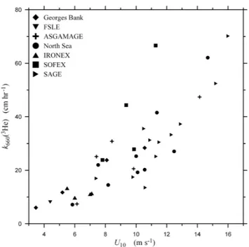
Fig. 1. Available oceanic measurements of the air-sea gas transfer velocity made using the purposeful dual-tracer method normalized to a common Schmidt number of 660,k660(3He), plotted as a
func-tion of wind speed. The data key is shown on the figure. In the key: Georges Bank is data from Wanninkhof et al. (1993); FSLE is data from Wanninkhof et al. (1997); ASGAMAGE is data from Jacobs et al. (1999); North Sea is data from Nightingale et al. (2000b), IRONEX is data from Nightingale et al. (2000a); SOFEX is data from Wanninkhof et al. (2004); and SAGE is data from Ho et al. (2006).
However, it is less clear that field measurements ofkLcan be
easily partitioned into those made under surfactant-impacted conditions and those made under so-called clean conditions. Even more uncertain is how to best parameterize the role of turbulence in influencing the magnitude ofkL.
Under most conditions, the wind stress plays a dominant role in providing the turbulence kinetic energy involved in promoting gas exchange. Therefore, wind speed,U, has long been used to parameterizekL. Figure 1 showskLmeasured
in the ocean using the purposeful dual-tracer method (Wat-son et al., 1991) plotted as a function ofU. (The data in the figure were compiled from Wanninkhof et al. (1993, 1997, 2004), Jacobs et al. (1999), Nightingale et al. (2000a, b) and Ho et al. (2006) and have all been scaled to a common dif-fusivity equal to carbon dioxide in seawater at 293.15 K, de-fined here in terms of the Schmidt number (660), assuming that kL is proportional to D1/2). When the values for the
scaled transfer velocity,k660, at a particularUare compared, the data are considerably scattered. It can be argued that the overall dependence follows either a polynomial dependence or a segmented linear dependence withU. Unfortunately, there is too much scatter in the data to allow the data to pro-vide a definitive selection between any of the available gas exchange parameterizations.
Figure 1 typifies the problem in attempting to develop a method for accurately estimatingkLfrom an easily measured
environmental parameter. The data in the figure represent measurements of the highest quality, collected by meticu-lous and careful groups. Because of this, it is assumed that much of the scatter in the data represents variability in the transfer velocity imposed by variability in the environmental conditions. This could occur if, for example, the levels of aqueous-phase turbulence generated at a particular value of
U depend on factors other than theU itself. This explana-tion seems logical on an intuitive level, but the fundamental measurements of near-surface oceanic turbulence necessary to support it are not available. So it could be that the scat-ter in Fig. 1 could simply represent experimental uncertainty rather than environmental variability.
The purpose of this paper is to explore whether it is pos-sible to explain the scatter in various measurements of the
kLsimply in terms of the uncertainty in measuring the
un-derlying parameters. This will be done using the dual-tracer data shown in Fig. 1 and using gas transfer data collected in a wind-wave tunnel.
2 Theory
In the case where a non-reactive gaseous tracer is injected into a known volume of water, the change in concentration with respect to time due to the water-to-air gas flux can be written as
dCB
dt = kLA
V (KHPA−CB) (1)
where CB is the bulk-phase concentration of the tracer
gas (mol m−3), A is the surface area of the water through which gas exchange occurs (m2), V is the total water vol-ume (m3), KH is the aqueous-phase solubility of the gas
(mol m−3kPa−1), andPA is the partial pressure of the gas
in the air phase (kPa). The productKHPA defines the
equi-librium saturation concentration of the gas,CS. Integration
of Eq. (1) shows thatkLcan be written as
kL=
V A 1t ln
C S−C0
CS−CB
(2) where1t is the time difference andC0is the concentration of the tracer gas at timet = 0. From Eq. (2), a plot of the quantity−ln((CS−C0)/(CS−CB) versus time will result in a
straight line with slope equal tokLA/V.
A similar relation exists for the analysis of purposeful dual-tracer method (PDTM) data collected during oceanic air-sea gas exchange measurements. In these experiments, the two volatile tracer gases sulfur hexafluoride (SF6) and helium-3 (3He) are injected into the surface mixed layer. Their concentrations are then measured as a function of time and the transfer velocity of3He,kL(3He), can be estimated
Fig. 2. The air-water gas transfer velocity for He normalized to Sc=600,k660(He), measured during FEDS plotted as a function of
wind speed. Also shown are values fork660(He)AVGproduced by
the Monte Carlo model described in Sect. 3. The data key is shown on the figure. The dashed lines represent the values bounding 90% of thek660(He)AVGvalues produced by the Monte Carlo model.
If the atmospheric concentration of both gases is assumed to be zero (Wanninkhof et al., 1993), this relation has the form
kL
3He= −h 1t1
(
ln
3He
[SF6]
!)
1− "
Sc 3He Sc(SF6)
#1/2
−1
(3)
where h is the mixed layer depth, 1t is the time in-terval over which the change in concentrations are mea-sured, [3He] and [SF6] are the concentrations of 3He and SF6, respectively, and Sc(3He) and Sc(SF6) are the Schmidt numbers of 3He and SF6, respectively. In specific, the term 1{ln([3He]/[SF6])} in Eq. (3) should be interpreted as ln([3He]t2/[SF6]t2) – ln([
3He]
t1/[SF6]t1) where the
sub-scriptst1andt2imply the concentrations measured at times
t1andt2, respectively. The “dual-tracer term” defined by 1-[Sc(3He)/Sc(SF6)]1/2is 0.64 at 278 K for seawater and 0.61 at 298 K using Sc(3He) calculated as outlined in J¨ahne et al. (1987) and Sc(SF6) from King and Saltzman (1995)
Applying either Eq. (2) or (3) is straightforward and the theoretical basis for each are not in dispute (with possible exception being the correct value of the exponent for the Schmidt number term). However, because of the logarithmic relationship involving the concentrations and the fact that the change in concentration with respect to time can be relatively small, both equations are sensitive to measurement uncer-tainty.
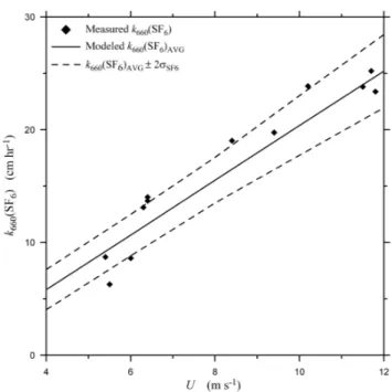
Fig. 3. The air-water gas transfer velocity for SF6normalized to
Sc=660,k660(SF6), measured during FEDS plotted as a function of
wind speed. Also shown are values fork660(SF6)AVGproduced by
the Monte Carlo model described in Sect. 3. The data key is shown on the figure. The dashed lines represent the values bounding 90% of thek660(SF6)AVGvalues produced by the Monte Carlo model.
In laboratory experiments, it is common to simultaneously measurekLfor several gases. From these data, it is possible
to estimate the dependence ofkL on molecular diffusivity.
Conceptual models for air-water gas transfer assume that this dependence can be written as
kL=a ν
D
−n
f (Q, L) (4)
whereaandnare constants,νis the kinematic viscosity of water, andf (Q,L)symbolizes the as yet unspecified depen-dence ofkLon the turbulence velocity and length scales. The
ratioν/Dis the Schmidt number, Sc, and it will be used from this point in place ofD. Depending on the conceptual model,
ncan range from 1/2 to 2/3 with the lower value usually as-sociated with gas exchange through a clean water surface and higher values associated with transfer through surfactant in-fluenced surfaces. Therefore, the dependence of kL on Sc
provides very useful information on the transfer process and it is highly desirable to be able to estimatenfrom experimen-tal data.
Using Eq. (4), it can be shown that if thekLvalues for two
gases with different Sc numbers are known,nis equal to
n= ln [kL(1) / kL(2)]
134 W. E. Asher: Experimental error and air-sea gas exchange where the (1) and (2) refer to the parameter for the two
re-spective gases. As is the case for calculatingkLitself, Eq. (5)
is also sensitive to measurement errors because Sc for most gases does not vary by a large amount.
3 Wind-wave tunnel measurements
The Flux Exchange Dynamics Study (FEDS) was conducted in 1998 at the Air-Sea Interaction Research Facility (ASIRF) wind-wave tunnel at the US National Aeronautics and Space Agency, Goddard Space Flight Center, Wallops Flight Facil-ity in Wallops Island, Virginia. These measurements have been described in detail elsewhere (Zappa et al., 2004) and only a brief description will be provided here. During the study,kLwas measured for SF6and helium (He) using gas
chromatography to determine aqueous-phase gas concentra-tions. Method precision for measuring gas concentrations was found to be±3% for SF6and±7% for He. Figure 2 shows transfer velocities for He normalized to Sc=660 as-sumingn=1/2,k660(He), measured during FEDS plotted as a function of wind speed,U. Figure 3 shows transfer veloci-ties measured during FEDS for SF6normalized to Sc=660,
k660(SF6), also plotted versus U. Sc values for SF6 were taken from King and Saltzman (1995) and Sc for He was taken from Wanninkhof (1992). Uncertainty in Sc(He) is 2.1% (J¨ahne et al., 1987) and 4.2% for Sc(SF6) (King and Saltzman, 1995), although uncertainties in Sc were neglected here since they will not affect the variability in the resulting transfer velocities.
As was seen in the field data in Fig. 1, there is some scat-ter in the measured values of the transfer velocity when plot-ted versusU. However, in contrast to the field data,kL in
the wind-wave tunnel increases approximately linearly with
U. What is not clear from the data is whether the scatter in
kLreflect experimental noise or day-to-day variability in the
conditions affecting gas transfer in the wind tunnel. In or-der to unor-derstand the relative roles experimental uncertainty and environmental variability play in governing the scatter in measuredkL values, a Monte Carlo-type simulation was
performed using the known experimental uncertainties to es-timate the variability inkLthat would be expected given the
uncertainties in the gas concentrations.
The first step in this procedure was to use the experimen-tal data in Figs. 2 and 3 to produce a linear relation for esti-matingkLfrom wind speed in the ASIRF wind-wave tunnel.
Least-squares linear regression of the combined gas transfer data set showed thatkLat a particular value of Sc,kL(Sc),
could be calculated as
kL(Sc)=
660 Sc
1/2
(6.73U−10.76) (6)
for kL(Sc) in µm s−1 and U in m s−1 with the coefficient
of determination for the regression being 0.91 and a stan-dard error of the fit equal to 5.29µm s−1. Then, Eq. (2) was rewritten in the form
CB =CB−(CS−C0)exp
−A kL(Sc) t
V
(7) so that gas concentrations for a gas with a particular Schmidt number could be predicted as a function oft. Concentrations for He and SF6were predicted at five times with time steps on the order of 2000 s so that the number of modeled concen-trations and their time steps were equal to the experimental sampling rate used in the actual experiments. (It should be noted that simulating experiments with extremely long time steps where gas concentrations decrease to within 10% of their equilibrium values greatly decreases the effect of mea-surement error.) Then, the predicted concentrations were modified by adding or subtracting a random amount deter-mined by the measurement error for that particular gas.
For the Monte Carlo simulations, 1000 separate sets of concentrations with independent experimental uncertain-ties were produced for each gas at U = 4 m s−1, 6 m s−1, 8 m s−1, 10 m s−1, and 12 m s−1. These concentrations were then used in Eq. (2) to calculate k660(SF6) and
k660(He). The mean value of the model-calculated trans-fer velocities,k660(He)AVGandk660(SF6)AVG, are shown in Figs. 2 and 3, respectively. Also shown in each figure are
k660(He)AVG±2σHe andk660(SF6)AVG±2σSF6 at each wind speed, or the bounds showing range of 90% of the model-derivedkLvalues (i.e., 900 out of the 1000 calculated
trans-fer velocities at each U lie within the dashed lines in each figure).
The fraction of the total observed variability that is ex-plained by measurement errors can be estimated by calculat-ing the standard errors in the experimental and simulated data sets. A least-squares linear regression of thekLvalues from
the Monte Carlo simulations for each gas gives a standard error of the fit of 1.2 for SF6and 1.1 for He. A least-squares linear regression of the experimental data for each gas gives standard errors of the fit of 2.3 and 1.9 for SF6and He, re-spectively. Taking the ratios of these values shows that the experimental measurement uncertainty explains 53% of the observed experimental variability for SF6and 58% of the ex-perimental variability for He. This indicates that half of the variability in thekLvalues is due to concentration
measure-ment precision and not day-to-day changes in uncharacter-ized environmental conditions in the wind-wave tunnel.
be close to unity, making the logarithm small which ampli-fies the effect of the measurement error. Because Sc(SF6) is larger than Sc(He) by a factor of 8 and the transfer velocity scales as Sc−1/2, the concentration of SF6in the wind-wave tunnel decreases a little under half as fast as He. This means for an equivalent experimental time period, the effect of er-rors in concentration will have a larger effect on SF6than on He. The obvious solution to this problem is to run experi-ments over many hours so that both concentrations approach their equilibrium values. However, in situations where a set of gas transfer experiments must be conducted over a time span of a few days in a particular facility, running experi-ments for periods longer than a few hours can cause logistical complications.
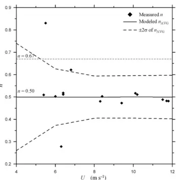
The modeled concentrations can also be used to study the variability in values ofndeduced from measurements ofkL.
Figure 4 showsncalculated using Eq. (5) andkL(SF6) and
kL(He) measured in the wind-wave tunnel plotted vesusU.
Also shown in Fig. 4 is the average Schmidt number expo-nent,nAVG, calculated using the gas transfer velocities calcu-lated from the Monte Carlo simulation above and Eq. (5). As expected for a clean surface,nAVG=1/2. Of more interest is the range innAVG, here expressed asnAVG±2σnwhereσnis
the standard deviation of the 1000nvalues from the Monte Carlo simulation. The range innAVG±2σnspans the
variabil-ity inncalculated from the wind-tunnel data. This suggests that the variability observed in Fig. 4 is not due to environ-mental variability and merely reflects the sensitivity ofnto the experimental uncertainty in calculatingkL.
In the above analysis of the variability inn, it was assumed thatn was equal to 1/2 and constant as a function of wind speed. However, laboratory data exists suggesting thatnis a function ofU, decreasing from 2/3 to 1/2 asU increases (J¨ahne et al., 1984; Zappa et al., 2004). Since understanding the dependence ofkLonnis important in determining a
cor-rect conceptual model for air-water gas transfer (Atmane et al., 2004) and in analyzing results from oceanic dual-tracer gas exchange experiments, it is often the case that gas trans-fer measurements are used to determine the dependence ofn
onU.
The Monte Carlo method described above was used to as-sess how measurement errors might affect determining the functionality ofnwith respect toU. First, it was assumed thatnwas given by
n=0.67: U <2m s−1
n=0.5+0.17 exp−U2−2: U≥2m s−1 (8)
and then kL values were calculated for the gases methane
(CH4), SF6, and He using Eq. (6) usingncalculated using Eq. (8) in place of the exponent 1/2. Sc values for CH4were taken from Wanninkhof (1992). Transfer velocities were cal-culated at U=3 m s−1, 4 m s−1, 6 m s−1, 8 m s−1, 10 m s−1, and 12 m s−1. As before, 1000 concentration time series that included a±3% random error and had time steps as given
Fig. 4. The Schmidt number exponent,n, calculated using Eq. (5) and gas transfer velocity data for the gas pair SF6and He measured
in the Wallops Flight Facility wind/wave tunnel. Also shown in the figure is the averagen,nAVG, and range ofncalculated using the
Monte Carlo method and 1000 trial runs. The data key is shown on the figure whereσ is the standard deviation of the modeledn
values.
above in each value were generated for each gas. Then,kL
was calculated using each concentration time series. An esti-mate ofncould then be derived using the gas pairs CH4/SF6, CH4/He, and SF6/He. Figure 5 showsnAVGandnAVG±2σn
for all three gas pairs.
The choice of functional form for Eq. (8) was selected be-cause it approximates the measured dependence of n as a function ofU (J¨ahne et al., 1984; Zappa et al., 2004). The-oretical justification for assuming nwill decrease asU in-creases can be made through heuristic appeals to eddy struc-ture models for air-water gas transfer (Harriott, 1962). In these models, as the penetration depths and timescales of turbulence eddies at the water surface decrease,ndecreases from a maximum of 1 to a lower limit of 1/2 – see Fig. 3 of Harriott (1962). Because it is known that penetration depth and timescales decrease with increasing levels of turbulence (Asher and Pankow, 1991a, b) and it is known that turbulence increases with increasing wind speed (Siddiqui et al., 2004), it is reasonable to assume thatnwill decrease monotonically to the lower limit of 1/2 asUincreases.
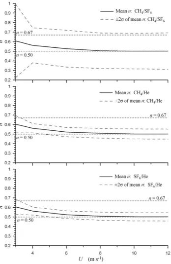
The top panel in Fig. 5 shows the results for CH4/SF6. Be-cause the change in Sc value for these two gases is relatively small (e.g., Sc(CH4) = 616 @ 293.15 K, Sc(SF6) = 948 @ 293.15 K), the calculation ofnis very sensitive to measure-ment error so the±2σnrange is large and if only a few
136 W. E. Asher: Experimental error and air-sea gas exchange
Fig. 5.Plots of the expected experimental variance in Sc exponent
ncalculated using Eq. (5) and transfer velocities from the Monte Carlo procedure described in the text plotted as a function of wind speed,U, for the gas pairs: methane (CH4) and sulfur hexafluoride
(SF6), top panel; CH4and helium (He), middle panel; and He and SF6, bottom panel. The model assumes the uncertainties in gas
concentrations are uncorrelated. The data key for each is shown on each figure.
ngiven by Eq. (8) would result. The situation improves for both gas pairs involving He, mainly because Sc(He) = 149 at 293.15 K. However, the variability in the calculatedn val-ues is still large and accurately resolving the dependence of
non wind speed would require a significant number of ex-periments be conducted.
4 Oceanic purposeful dual-tracer measurements
The Monte Carlo method described in the previous section can also be applied to the purposeful dual-tracer method PDTM. However, in the case of PDTM data analysis, in ad-dition to the measurement uncertainties in the gas concen-trations, the uncertainty in the mixed layer depth, h, must
also be taken into account. As discussed by Wanninkhof et al. (2004), the analysis of PDTM data proceeds by analyzing discrete segments of a times series of concentrations for the two gases over intervals where the wind speed was relatively constant. Although nonsteady wind speeds are recognized as having an effect on PDTM analysis (Wanninkhof et al., 2004), including variable wind speeds is beyond the scope of this paper and this study will assume steady wind speeds.
For the simulations performed here, it was assumed that the concentrations of both SF6and3He could be measured in the ocean with a precision of±2% (R. Wanninkhof, NOAA Atlantic Oceanographic and Meteorological Laboratory, Mi-ami Florida, personal communication). Defining the uncer-tainty inh is more problematic, especially considering that there have been two distinct types of oceanic PDTM ex-periments conducted. PDTM exex-periments have been con-ducted in well-mixed shallow-water coastal environments, where the mixed-layer depth is defined by the water depth (e.g., Wanninkhof et al., 1993; Watson et al., 1991). In these cases, where depth is typically measured using an ADCP, the uncertainty inhis due to tides and averaging over the depth bin in the ADCP. Therefore, the resulting uncertainties inh
are on order of±10%. More recently, PDTM experiments have been conducted in the open ocean, wherehis defined as the depth of the mixed-layer (Ho et al., 2006; Nightingale et al., 2000a; Wanninkhof et al., 1997, 2004). In these cases the uncertainty inhwas assumed to be±20% based on the uncertainty in extracting the mixed-layer depth from CTD profiles (D. Ho, University of Hawaii, personal communica-tion).
Unfortunately, the precision in gas concentration analysis for the oceanic dual-tracer data is different than the precision in concentration analysis for the wind-tunnel data discussed above. This makes direct comparison of the data problem-atic, but because of differences in instrumentation and analyt-ical techniques, it is not correct to use the same experimental precisions for each set of experiments.
The Monte Carlo simulations were carried out by calcu-lating the transfer velocities of SF6 and He, kL(SF6) and
kL(He), respectively, at for U = 4 m s−1, 8 m s−1, 12 m s−1
and 16 m s−1using theU2power law dependence proposed by Wanninkhof (1992). Assuming thath = 50 m (and that
A/V = 1/h)allowed Eq. (7) to be used with thesekLvalues
to generate concentrations for SF6and3He at discrete times. Concentration pairs were calculated att=0 and at times with
1t in the range of 1–2 days that included the independent measurement uncertainties. Then, an experimental h was chosen that included the effect of uncertainty. The h and concentrations were used in Eq. (3) to calculatekL(3He). As
was done previously, 1000 sets of concentrations were gen-erated at eachUand a mean transfer velocity normalized to Sc = 660,k660(3He)AVG, and associated standard deviation,
Fig. 6a. Air-sea gas transfer velocities of helium-3 normalized to Sc=660,k660(3He), measured using the purposeful dual-tracer
method in deep-water open ocean environments. Also shown are
k660(3He) values produced by the Monte Carlo simulations
de-scribed in Sect. 4. The data key is shown on the figure. Refer to the caption of Fig. 1 for explanation of experimental codes.
experiments and a separate set ofk660(3He) values were cal-culated using an uncertainty inhof ±20% to simulate the open ocean PTDM experiments. Figure 6 shows the data from Fig. 1 separated in the coastal and open-ocean PTDM experiments along with thek660(3He)AVG, and the range of the model results given ask660(He)AVG±2σ3Hecalculated us-ing the relevant uncertainties in the gas concentrations andh. Following the data analysis for the wind-wave tunnel data in the previous section, a least-squares regression of all the coastal PDTM field measurements in Fig. 6a (i.e., the North Sea, Georges Bank, FSLE, and ASGAMAGE data sets) of
k660(3He) versusU2gives a standard error of the fit of 7.0. A least-squares regression of all thek660(3He) values from the Monte Carlo simulation with a 10% uncertainty inhgives a standard error of the fit of 3.0. Therefore, these results indicate that 43% of the observed variability in the coastal PDTM results is due to uncertainty in gas concentrations and
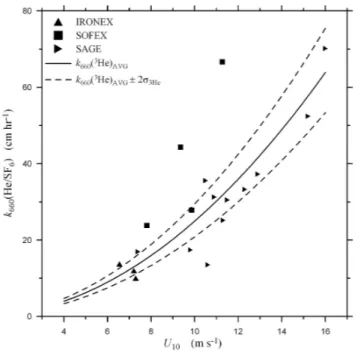
h. In the case of the open-ocean deep-water PDTM experi-ments in Fig. 6b (i.e., the IRONEX, SAGE, and SOFEX data sets), the standard error of the fit of the experimental data is 11.2. The regression of the Monte Carlo simulations run with a 20% uncertainty inhgives a standard error of 4.9, which indicates that 44% of the observed variability is explained by the measurement uncertainties in the concentrations and
h(interestingly, if the SOFEX data set is excluded from this analysis, the experimental standard error for the PDTM data decreases to 5.9 and the fraction of the error explained by
Fig. 6b. Air-sea gas transfer velocities of helium-3 normalized to Sc=660,k660(3He), measured using the purposeful dual-tracer
method in shallow-water coastal environments. Also shown are
k660(3He) values produced by the Monte Carlo simulations
de-scribed in Sect. 4. The data key is shown on the figure. Refer to the caption of Fig. 1 for explanation of experimental codes.
the measurement errors rises to 83%). This suggests that en-vironmental variability may not play as large a role as sup-posed, and that measurement uncertainty may account for approximately half of the observed scatter in the field mea-surements. Given the large difference between the precision of the gas concentration measurements andh, it is was found that uncertainty inhhas the largest effect onkL(3He). In
par-ticular,haccounts for 72% of the standard error in the mod-eled transfer velocities for the open-ocean deep-water runs and 57% of the standard error for the coastal runs.
5 Conclusions
138 W. E. Asher: Experimental error and air-sea gas exchange of the data in Fig. 1 is close to the “true” functional
depen-dence ofkLon wind speed. In turn, this is relatively good
news for those who hope to develop a robust method for pa-rameterizing gas transfer in terms of an easily measured envi-ronmental variable. However, it also points out the difficulty associated with making the measurements used to validate these parameterizations, especially in regards to determining the functional dependence ofkLon Schmidt number.
Specific recommendations for reduction of variability in laboratory experiments include reducing measurement errors in gas concentrations, since these errors can account for half of the observed variability in the transfer velocities. This is especially true when conducting experiments designed to determinen. In cases where increasing the precision of the concentration measurements is not possible, increasing the length of time over which concentration decreases are mea-sured reduces the effect of uncertainty in concentrations.
In the case of PDTM experiments conducted in stratified waters, where the mixed layer depth must be determined by CTD cast or other method, these results show that transfer ve-locities are particularly sensitive to uncertainty inh. In these cases reducing the uncertainty in concentrations would have little effect on the experimental noise and particular attention should be paid to measuring the mixed-layer depth. The re-sults from PDTM experiments conducted in well-mixed shal-low waters show a higher fraction of the observed experimen-tal variability that is not accounted for by the measurement uncertainties. This suggests that the effects of variability in the forcing mechanisms are higher in these situations, and particular emphasis should be placed on measuring the forc-ing functions for gas exchange such as wind stress and wave breaking.
Acknowledgements. This work was funded by the National Science Foundation under grant OCE-0425305. The comments of the referees were very helpful in preparation of this paper and I thank them for their input.
Edited by: J. Kaiser
References
Asher, W. E. and Litchendorf, T. M.: Visualizing near-surface CO2 concentration fluctuations using laser-induced fluorescence, Exp. in Fluids, doi:10.1007/s00348-008-0554-9, in press, 2009. Asher, W. E. and Pankow, J. F.: The effect of surface films on
con-centration fluctuations close to a gas/liquid interface, in: Air-Water Mass Transfer, edited by: Wilhelms, S. E., and Gulliver, J. S., American Society of Civil Engineering, New York, 68–80, 1991a.
Asher, W. E. and Pankow, J. F.: Prediction of gas/water mass trans-port coefficients by a surface renewal model, Env. Sci. Tech., 25, 1294–1300, 1991b.
Atmane, M. A., Asher, W. E., and Jessup, A. T.: On the use of the active infrared technique to infer heat and gas transfer
veloc-ities at the air-water free surface, J. Geophys. Res.-Oceans, 109 (C08S14), doi:10.1029/2003JC001805, 2004.
Davies, J. T.: Turbulence Phenomena, Academic Press, New York, 412 pp., 1972.
Frew, N. M., Goldman, J. C., Dennett, M. R., and Johnson, A. S.: Impact of phytoplankton-generated surfactants on air-sea gas ex-change, J. Geophys. Res.-Oceans 95C, 3337–3352, 1990. Harriott, P.: A random eddy modification of the penetration theory,
Chem. Eng. Sci. 17, 149-154, 1962.
Herlina and Jirka, G. H.: Application of LIF to investigate gas trans-fer near the air-water interface in a grid-stirred tank, Exp. Fluids, 37(3), 341–349, 2004.
Herlina and Jirka, G. H.: Experiments on gas transfer at the air-water interface induced by oscillating grid turbulence, J. Fluid Mech. 594, 183–208, 2008.
Ho, D. T., Law, C. S., Smith, M. J., Schlosser, P., Harvey, M., and Hill, P.: Measurements of air-sea gas exchange at high wind speeds in the Southern Ocean: Implications for global parameterizations, Geophys. Res. Lett., 33 L16611, doi:10.1029/2006GL026817, 2006.
Jacobs, C., Kjeld, J. F., Nightingale, P., Upstill-Goddard, R., Larsen, S., and Oost, W.: Possible errors in CO2 air-sea transfer veloc-ity from deliberate tracer releases and eddy covariance measure-ments due to near-surface concentration gradients, J. Geophys. Res.-Oceans 107 (L3128), doi:10.1029/2001JC000983, 2002. Jacobs, C. M. J., Kohsiek, W., and Oost, W. A.: Air-sea fluxes and
transfer velocity of CO2 over the North Sea: results from AS-GAMAGE, Tellus B, 51(3), 629–641, 1999.
J¨ahne, B., Heinz, G., and Dietrich, W.: Measurement of the diffu-sion coefficients of sparingly soluble gases in water, J. Geophys. Res.-Oceans 92, 10 767–10 776, 1987.
J¨ahne, B., Huber, W., Dutzi, A., Wais, T., and Ilmberger, J.: Wind/wave tunnel experiments on the Schmidt number and wave field dependence of air-water gas exchange, in: Gas Transfer at Water Surfaces, edited by: Brutsaert, W. and Jirka, G. H., Reidel, Dordrecht, 303–310, 1984.
King, D. B. and Saltzman, E. S.: Measurement of the diffusion coef-ficient of sulfur hexafluoride in water, J. Geophys. Res.-Oceans, 100, 7083–7088, 1995.
McGillis, W. R., Edson, J. B., Hare, J. E., and Fairall, C. W.: Di-rect covariance air-sea CO2 fluxes, J. Geophys. Res.-Oceans, 106(C8), 16 729–16 745, 2001a.
McGillis, W. R., Edson, J. B., Ware, J. D., Dacey, J. W. H., Hare, J. E., Fairall, C. W., and Wanninkhof, R. Carbon dioxide flux techniques performed during GasEx-98, Mar. Chem., 75, 267– 280, 2001b.
McGillis, W. R., Edson, J. B., Zappa, C. J., Ware, J. D., McKenna, S. P., Terray, E. A., Hare, J. E., Fairall, C. W., Drennan, W., Donelan, M., DeGrandpre, M. D., Wanninkhof, R., and Feely, R. A.: Air-sea CO2 exchange in the equatorial Pacific, J. Geophys. Res.-Oceans, 109, 2004.
McKenna, S. P. and McGillis, W. R.: The role of free-surface turbu-lence and surfactants in air-water gas transfer, Int. J. Heat Mass Trans., 47(3), 539–553, 2004.
M¨unsterer, T. and J¨ahne, B.: LIF measurements of concentration profiles in the aqueous mass boundary layer, Exp. Fluids, 25, 190–196, 1998.
Res. Lett., 27(14), 2117–2120, 2000a.
Nightingale, P. D., Malin, G., Law, C. S., Watson, A. J., Liss, P. S., Liddicoat, M. I., Boutin, J., and Upstill-Goddard, R. C.: In situ evaluation of air-sea gas exchange parameterizations using novel conservative and volatile tracers, Global Biogeochem. Cy., 14, 373–387, 2000b.
Siddiqui, M. H. K., Loewen, M. R., Asher, W. E., and Jessup, A. T.: Coherent structures beneath wind waves and their influence on air-water gas transfer, J. Geophys. Res.-Oceans 109, C03024, doi:03010.01029/02002JC001559, 2004.
Wanninkhof, R.: Relationship between wind speed and gas ex-change over the ocean, J. Geophys. Res.-Oceans, 97, 7373–7382, 1992.
Wanninkhof, R., Asher, W. E., Weppernig, R., Chen, H., Schlosser, P., Langdon, C., and Sambrotto, R.: Gas transfer experiment on Georges Bank using two volatile deliberate tracers, J. Geophys. Res.-Oceans, 98, 20 237–20 248, 1993.
Wanninkhof, R., Hitchcock, G., Wiseman, W., Ortner, P., Asher, W., Ho, D., Schlosser, P., Dickson, M.-L., Anderson, M., Masserini, R., Fanning, K., and Zhang, J.-Z.: Gas exchange, dispersion, and biological productivity on the west Florida shelf: Results from a Lagrangian tracer study, Geophys. Res. Lett., 24, 1767–1770, 1997.
Wanninkhof, R., Sullivan, K. F., and Top, Z. Air-sea gas transfer in the Southern Ocean, J. Geophys. Res.-Oceans, 109, C08S19, doi:10.1029/2003JC001767, 2004.
Woodrow Jr., P. T., and Duke, S. R.: Laser-induced fluorescence studies of oxygen transfer across unsheared flat and wavy air-water interfaces, Ind. Eng. Chem. Res., 40, 1985–1995, 2001. Zappa, C. J., Asher, W. E., Jessup, A. T., Klinke, J., and Long,