doi:10.5194/bg-9-957-2012
© Author(s) 2012. CC Attribution 3.0 License.
Sea-to-air and diapycnal nitrous oxide fluxes in the eastern tropical
North Atlantic Ocean
A. Kock1, J. Schafstall2, M. Dengler2, P. Brandt2, and H. W. Bange1
1Forschungsbereich Marine Biogeochemie, Helmholtz-Zentrum f¨ur Ozeanforschung Kiel (GEOMAR), Germany 2Forschungsbereich Ozeanzirkulation und Klimadynamik, Helmholtz-Zentrum f¨ur Ozeanforschung Kiel (GEOMAR),
Germany
Correspondence to:A. Kock (akock@geomar.de)
Received: 12 October 2011 – Published in Biogeosciences Discuss.: 20 October 2011 Revised: 23 February 2012 – Accepted: 23 February 2012 – Published: 7 March 2012
Abstract. Sea-to-air and diapycnal fluxes of nitrous oxide (N2O) into the mixed layer were determined during three
cruises to the upwelling region off Mauritania. Sea-to-air fluxes as well as diapycnal fluxes were elevated close to the shelf break, but elevated sea-to-air fluxes reached further off-shore as a result of the offoff-shore transport of upwelled water masses. To calculate a mixed layer budget for N2O we
com-pared the regionally averaged sea-to-air and diapycnal fluxes and estimated the potential contribution of other processes, such as vertical advection and biological N2O production in
the mixed layer. Using common parameterizations for the gas transfer velocity, the comparison of the average sea-to-air and diapycnal N2O fluxes indicated that the mean
sea-to-air flux is about three to four times larger than the diapyc-nal flux. Neither vertical and horizontal advection nor bio-logical production were found sufficient to close the mixed layer budget. Instead, the sea-to-air flux, calculated using a parameterization that takes into account the attenuating ef-fect of surfactants on gas exchange, is in the same range as the diapycnal flux. From our observations we conclude that common parameterizations for the gas transfer velocity likely overestimate the air-sea gas exchange within highly produc-tive upwelling zones.
1 Introduction
Nitrous oxide (N2O) is a potent greenhouse gas with a major
contribution of oceanic emissions to its atmospheric budget (Denman et al., 2007). It is produced in the oxic subsur-face and deep ocean during microbial nitrification, whereas in anoxic to suboxic parts of the ocean N2O can be produced
and/or consumed during canonical denitrification (see e.g. Castro-Gonzalez and Farias, 2004; Nicholls et al., 2007).
While large parts of the surface ocean are close to equilib-rium with the atmosphere, enhanced emissions are observed during coastal upwelling events due to the transport of N2
O-enriched subsurface waters into the mixed layer (ML, see e.g. Nevison et al., 2004). Pronounced coastal upwelling in the eastern tropical North Atlantic Ocean (ETNA) occurs sea-sonally along the coasts of Mauritania and Senegal. Con-sistently, N2O emissions are found to be enhanced during
winter/spring (Wittke et al., 2010).
In this study we quantify the diapycnal and sea-to-air fluxes of N2O in the ETNA (incl. the upwelling off
Mau-ritania) to estimate the contribution of diapycnal mixing to the N2O ML budget: N2O concentrations in the ML should,
at steady state, represent the balance between physical pro-cesses such as vertical mixing, air-sea gas exchange with the overlying atmosphere, vertical and horizontal advection and, potentially, biological processes such as nitrification. The relative importance of the different terms for the N2O ML
budget is discussed. It is found that diapycnal and sea-to-air fluxes are the leading terms in the N2O ML budget and
sea-to-air fluxes are likely overestimated when using common parameterizations for the gas transfer velocity.
2 Study site
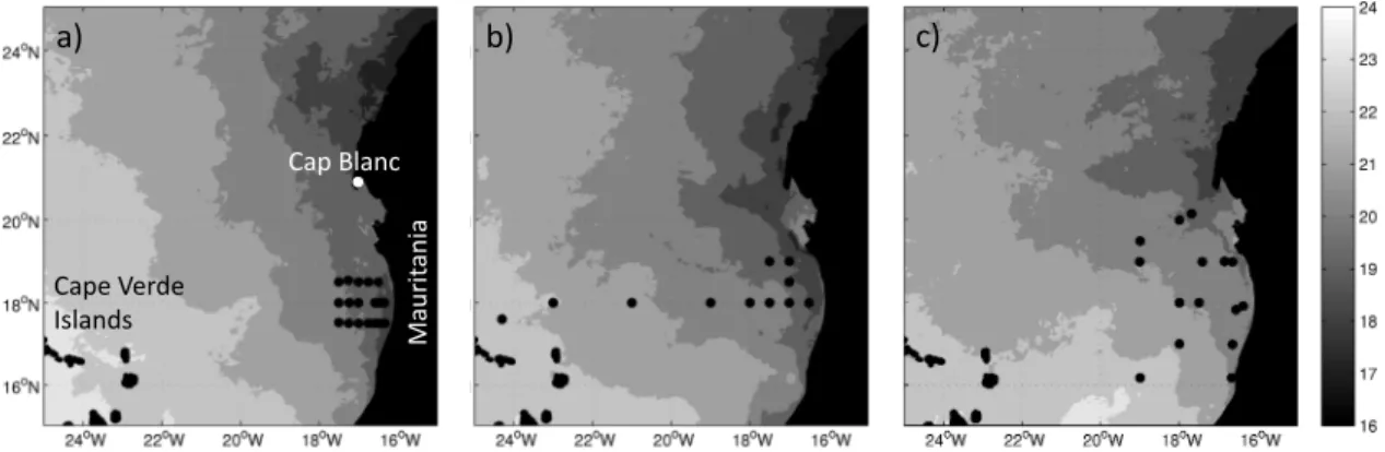
The investigated area covers the ETNA between the Cape Verde Islands and coast of Mauritania (Fig. 1). A lack of river inputs combined with a narrow continental shelf mini-mizes additional contributions of N2O originating from
Mauri
tani
a
Cap Blanc
Cape Verde Islands
a) b) c)
Fig. 1.Map with locations of the sampled stations during P347 in January 2007(a), P348 in February 2007(b)and ATA3 in February 2008 (c). MODIS monthly sea surface temperatures (in◦C) are also shown (http://oceandata.sci.gsfc.nasa.gov/MODISA/Mapped/). CVI stands for Cape Verde Islands.
the year (Hagen, 2001). In the region between Cap Vert (∼15◦N) and Cap Blanc (∼21◦N) seasonal upwelling takes place during winter/spring (Schemainda et al., 1975). Com-pared to other eastern boundary upwelling systems, the wa-ter column in the ETNA has relatively high oxygen con-centrations: minimum oxygen concentrations reach down to 40 µmol l−1 (Stramma et al., 2008). We thus conclude that the main production pathway for N2O in this region is
nitrification.
3 Methods
N2O concentration, microstructure and
conductivity-temperature-depth (CTD) measurements were conducted during three cruises to the ETNA (Fig. 1). The cruises were part of the German BMBF joint project SO-PRAN (Surface Ocean Processes in the Anthropocene, www.sopran.pangaea.de) and the DFG-funded Mauritanian upwelling and mixing process study (MUMP). They were scheduled in the upwelling season in January/February 2007 (R/VPoseidon cruises P347 and P348) and February 2008 (R/VL’Atalante cruise ATA3). Water samples were analyzed for dissolved N2O on board using a GC/ECD
system (Hewlett Packard 5890 II during ATA3, Carlo Erba HRGC 5160 Mega Series during P347 and P348) with a static equilibration method. The GCs were equipped with a 6′1/8′′ stainless steel column packed with molecular sieve (5 ˚A) (W. R. Grace & Co.-Conn., Columbia, MY) and oper-ated at a constant oven temperature of 190◦C (HP 5890II) and 220◦C (Carlo Erba HRGC 5160). Argon-methane (95/5, 5.0, AirLiquide, D¨usseldorf, Germany) was used as carrier gas at a flow rate of 30 ml min−1. Triplicates of bubble free samples were drawn from 10 l Niskin bottles mounted on a CTD/rosette, poisoned with mercuric chloride or measured within 24 h after sampling. For analysis, a 10 ml helium headspace was added to each sample using a gas-tight syringe (VICI Precision Sampling, Baton Rouge,
LA). A 9.5 ml subsample of the headspace was analyzed for nitrous oxide after an equilibration time of minimum 2 h. The GC was calibrated on a daily basis using at least two different standard gas mixtures (Deuste Steininger GmbH, M¨uhlheim, Germany) to account for potential drift of the detector. The concentration of N2O in the water
phase was calculated using the solubility function of N2O
from Weiss and Price (1980). The average precision of the measurements, calculated from error propagation, was
±0.7 nmol l−1.
N2O sea-to-air fluxesFsta(in nmol m−2s−1)were
calcu-lated from the gas exchange equation:
Fsta=kw·1N2O=kw·([N2O]w− [N2O]a) (1)
wherekwis the gas transfer velocity and [N2O]wis the
mea-sured in-situ concentration from the shallowest Niskin bottle in the surface layer (5–10 m). The N2O equilibrium
concen-tration [N2O]awas calculated by using a mean dry mole
frac-tion of 321 ppb (extracted from the monthly time series of at-mospheric N2O from the AGAGE monitoring station Ragged
Point on Barbados; see http://agage.eas.gatech.edu; Prinn et al., 1990) and the temperature and salinity at the depth of the corresponding Niskin bottle. kw was calculated using
thekw/wind speed relationships as defined by Nightingale et
al. (2000), Liss and Merlivat (1986) and Wanninkhof (1992) (Fig. 2). Wind speeds were obtained from the ships’ under-way observations for the calculation of the sea-to-air flux at the individual stations. For the calculation of regionally av-eraged sea-to air fluxes, we used three day mean QuikScat wind speeds (ftp://ftp.ssmi.com/qscat/).
Alternatively, the sea-to-air flux densities were calculated using the gas transfer velocity parameterization from Tsai and Liu (2003) that takes into account the reduction of the air-sea gas exchange due to surfactants (Fig. 2).
Fig. 2. Wind speed parameterizations used for the calculation of sea-to-air fluxes of N2O. The black lines represent gas exchange parameterizations for conditions without surfactants while the red line represents the parameterization of Tsai and Liu (2003) for surfactant-influenced surface waters.
profiler, a winch with a cable drum attached to the bulwark and a deck unit. The profilers used during the different cruises were equipped with two shear sensors (airfoil), a fast temperature sensor (FP07), an acceleration sensor, tilt sen-sors and standard CTD sensen-sors. They were adjusted to de-scent at a rate of 0.5–0.6 ms−1while the system records data from 16 channels at 1000 Hz. A detailed description of the instruments is given in Prandke and Stips (1998).
From the high-resolution shear measurements the dissipa-tion rates of turbulent kinetic energy (ε) were determined by integrating vertical wavenumber spectra of individual one-second ensembles assuming isotropy of turbulence at scales smaller than 0.6 m. Correction for unresolved spectral ranges and finite sensor tips were applied. For a detailed description of the algorithms used and the instrumental set up during the cruises the reader is referred to Schafstall et al. (2010).
Estimates of diapycnal N2O fluxes into the ML we
calcu-lated from the station-average diapycnal diffusivities derived from the microstructure measurements from 5 m below the ML depth to the depth of the next deeper N2O water sample.
Three to eight microstructure profiles were typically sampled at an individual station. ML depth was determined using the density criterion described by Kara et al. (2000). To avoid any influence from turbulence caused by the ship, the mini-mum ML depth was set to be at least 15 m deep. The diapyc-nal diffusivityKρwas computed according to Osborn (1980)
as
Kρ=Ŵ
ε
N2, (2)
and the diapycnal fluxesFdiaof N2O as
Fdia=Kρ·
d[N2O]
dz , (3)
with the local buoyancy frequencyN and the mixing effi-ciencyŴ which was set to a constant value of 0.2 (Oakey, 1982) and the vertical concentration gradientd[N2O]dz.
The local buoyancy was calculated from the profilers’ CTD measurements. Diapycnal N2O fluxes were determined
only from those microstructure profiles which were recorded concurrently with N2O profile sampling.
4 Results and discussion
To illustrate the N2O sea-to-air and diapycnal fluxes the
esti-mates from the individual stations were projected onto the distribution of topography along 18◦N (Fig. 3). For this comparison, wind speeds from the ship’s underway measure-ments were used to evaluate sea-to air fluxes. It should be noted that the comparison implicitly assumes that the mean fluxes have larger cross-shore than along-shore gradients, which was shown to be the case in the Mauritanian upwelling region by Schafstall et al. (2010).
The N2O sea-to-air fluxes using the Nightingale
et al. (2000) parameterization ranged from −0.02 to 0.5 nmol m−2s−1(Fig. 3). Highest fluxes were found close
to the shelf break in the zone of active upwelling indicated by low sea surface temperatures (SST). N2O sea-to-air fluxes
decreased with distance from the shelf break, which can be explained by a combination of continuous outgassing from N2O-enriched waters and its offshore transport within cold
filaments. The majority of the fluxes are positive indicating a flux of N2O from the ocean to the atmosphere. However,
we also computed negative fluxes which denote a N2O flux
from the atmosphere into the ocean. These negative fluxes correspond to1N2O values of max.−0.3 nmol l−1 and are
therefore within the uncertainty range of the measurements. The open ocean sea-to-air fluxes (west of 18◦W) are in agreement with the fluxes computed by Walter et al. (2006). The coastal fluxes between 18◦and 16◦W are, despite result-ing from a different approach, in reasonable agreement with the model-adjusted sea-to-air fluxes computed by Wittke et al. (2010). Rees et al. (2011) calculated sea-to-air fluxes from upwelling filaments of the Mauritanian upwelling in a simi-lar range to our results. Compared to other coastal upwelling systems, the average N2O fluxes from the Mauritanian
up-welling are relatively low (Charpentier et al., 2010; Bange et al., 1996).
The majority of the diapycnal N2O fluxes were lower than
the N2O sea-to-air fluxes from the Nightingale et al. (2000)
parameterization. Largest diapycnal fluxes were found in a narrow band in the region of the shelf break. However, enhanced fluxes were also encountered in the lower shelf region. Since the vertical N2O gradients were rather
uni-form, the variability of diapycnal fluxes is predominately due to the variability of diapycnal diffusivities (Kρ). As
Fig. 3. Diapycnal N2O (red dots, right axis) and sea-to-air fluxes (black dots, right axis) projected to 18◦N and bottom depth along 18◦N (solid line, left axis). Fluxes from stations to the north and south of 18◦N were projected onto 18◦N according to their dis-tance from the 400 m isobath.
Mauritanian upwelling is strongly enhanced due to presence of non-linear internal tides that form due to critically sloping topography (e.g. Holloway, 1985). Diapycnal nutrient fluxes calculated for the upwelling region are amongst the highest reported to date (Schafstall et al., 2010). Nevertheless, di-apycnal N2O fluxes from other coastal upwelling regions
re-ported by Charpentier et al. (2010) are in the same order of magnitude as the diapycnal fluxes inferred here.
To determine regional averages of the N2O sea-to-air
fluxes, the individual station estimates were extrapolated ex-ploiting the dependence of surface1N2O on SST anomaly
(Fig. 4). For this we used eight day mean MODIS Aqua SST data (http://oceandata.sci.gsfc.nasa.gov/MODISA/Mapped/ 8Day/4km/SST/) that covered the sampling periods.
The calculations were performed for an upwelling box off the Mauritanian coast. The size of the box was defined by the northernmost and southernmost sampled station, that is 20◦10′N and 16◦10′N respectively, the Mauritanian coast-line (except the Banc D’Arguin with bottom depths<10 m) and a line parallel to the shelf break located 170 km offshore. The SST anomaly was defined as the difference between the SST at a respective position in the upwelling box and the background SST averaged along a 100 km long section to the west of the box, thereby taking into account its mean lat-itudinal dependence.
Negative SST anomalies (SSTA) were significantly corre-lated with1N2O (r2= 0.54,n= 45; Fig. 4). A linear
regres-sion was used to calculate the regional surface1N2O
dis-tribution from the SSTA (1N2O =C·SSTA, with the slope
of the regression lineC=−2.82 nmol l−1◦C−1. 1N2O
val-ues from positive SST anomalies were set to zero, assum-ing that these values were not influenced by upwellassum-ing. The corresponding N2O sea-to air fluxes, calculated with the
Fig. 4. 1N2O vs. SST anomaly. The black line denotes the lin-ear regression of1N2O with respect to the SST anomaly for SST anomalies smaller than zero.
Nightingale (2000) parameterizantion, were calculated from three day mean QuikScat wind speeds (Fig. 6a). The re-sulting flux, averaged over the sampling period and the up-welling box, was 0.0685 (0.0677 to 0.0693) nmol m−2s−1. The confidence intervals were calculated using a Monte Carlo simulation with the uncertainties of the 1N2O
cali-bration and an assumed uncertainty of±2 m s−1for the wind
speed as input variables. To account for the large uncertain-ties in gas exchange velociuncertain-ties, we additionally calculated sea-to-air fluxes using the gas exchange parameterizations by Liss and Merlivat (1986) and Wanninkhof (1992) as lower and upper boundaries (Wanninkhof et al., 2009) (Table 1).
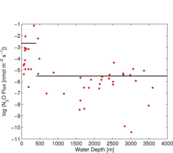
In contrast to the sea-to-air fluxes, the diapycnal fluxes were averaged in two regions according to their water depths: the shelf (water depth<400 m) and open ocean (water depth
≥400 m) region (Fig. 5). The average fluxes were 0.07 (0.025 to 0.126) nmol m−2s−1 for the shelf and 0.004 (0.002 to 0.007) nmol m−2s−1 for the open ocean region (Fig. 6b). This results in an overall average flux of 0.019 (0.007 to 0.048) nmol m−2s−1. Confidence intervals were calculated
from error propagation determined from the standard uncer-tainties ofε,N, mixing efficiencyγ and the vertical N2O
gradients as detailed in Schafstall et al. (2010).
Table 1.Sea-to-air fluxes (Fsta)of N2O calculated with different gas exchange parameterizations and corresponding N2O production rates
at a ML depth of 25 m required to compensate the discrepancy between the sea-to-air flux and the sum of diapycnal (Fdia)and vertical advective (Fadv)flux.
Parameterization Fsta[nmol m−2s−1] Fsta−(Fdia+Fadv) [nmol m−2s−1] Required N2O production rate [nmol l−1yr−1]
Nightingale (2000) 0.069 (0.067 to 0.070) 0.048 (0.018 to 0.060) 61 (22 to 76) Liss and Merlivat (1986) 0.047 (0.045 to 0.047) 0.026 (−0.005 to 0.038) 33 (−6 to 47) Wanninkhof (1992) 0.084 (0.082 to 0.085) 0.064 (0.032 to 0.076) 80 (41 to 95) Tsai and Liu (2003) 0.02 (0.019 to 0.021) −0.001 (−0.031 to 0.011) −1 (−40 to 14)
Fig. 5. Diapycnal N2O fluxes vs. water depth. The black lines denote average fluxes for the shelf and for the open ocean region.
The missing oceanic flux required to close the N2O ML
budget cannot be attributed to vertical advection of N2O
re-sulting from Ekman divergence, however. A regional av-erage of the vertical advective flux (Fadv) calculated from wind stress curl using QuikSCAT winds and N2O
concentra-tion differences between the ML and the next deeper avail-able value, from 10 to 30 m below the ML, resulted in 0.0021 nmol m−2s−1(Schafstall, 2010). Vertical advection of N2O is thus nearly an order of magnitude lower than the
diapycnal flux. Similarly, the horizontal flux divergence as-sociated with a mean N2O gradient along the eastern
bound-ary current is not able to close the N2O ML budget.
N2O production from near-surface nitrification has been
previously suggested to close the discrepancy between diapy-cnal and sea-to-air fluxes (e.g. Dore and Karl, 1996; Santoro et al., 2010). Recent publications have shown that nitrifica-tion within the euphotic zone can play a significant role in nutrient cycling of the surface ocean (Clark et al., 2008; San-toro et al., 2010; Wankel et al., 2007; Yool et al., 2007).
Based on the estimates of diapycnal, advective and sea-to-air flux we calculated potential N2O production rates closing
the N2O ML budget, assuming a ML depth of 25 m (Table 1).
Although covering a large range, the calculated N2O
produc-tion rates are extremely high: using the Nightingale (2000) parameterization, the average N2O ML production rate must
be as high as about 60 nmol kg−1yr−1 (0.16 nmol l−1d−1)
for a ML depth of 25 m. This exceeds N2O production
rates in the water column below the ML, quantified to be
≤3.3 nmol kg−1yr−1, by far (Freing et al., 2012). With a
molar N2O yield during nitrification between 0.5 and 0.01 %
(Bange, 2008) the corresponding nitrification rates would range from 30 to 1500 nmol l−1d−1. This is significantly higher than the nitrification rates of up to 5 nmol l−1d−1 from ML samples from Mauritanian upwelling region mea-sured by Clark et al. (2008) which, for comparison, would yield an N2O flux of 0.001 nmol m−2s−1at a N2O yield of
0.1 %.
In a more recent publication by Rees et al. (2011), nitrite oxidation rate measurements from two upwelling filaments off Mauritania provide higher nitrification rates in the up-per 100 m of the water column (25±12 nmol l−1d−1 and
115±106 nmol l−1d−1 for two different filaments), with a
tendency to increase with depth and maximum rates at 100 m depth.
Rees et al. (2011) compared the N2O production estimated
from their surface water nitrification rates with their sea-to-air fluxes and came the conclusion that surface N2O
produc-tion could only explain a small porproduc-tion of the sea-to-air flux of N2O. The majority of the N2O emissions would have to
be supplied from below.
Although these nitrification rates are high enough to make a substantial contribution to our mixed layer budget, this may be due to the different sampling strategy applied by Rees et al. (2011), who followed two upwelling filaments with strongly elevated primary productivity and N2O
a)
b)
c)
Fig. 6. (a)Regional distribution of the N2O fluxes calculated from SST anomalies and averaged over the sampling time using the Nightin-gale (2000) parameterization.(b)Regional distribution of the diapycnal N2O flux.(c)like(a)but using the Tsai and Liu (2003) parameteri-zation. Please note the different scaling of the colorbars in(a)and(b),(c).
Furthermore, their data provide another argument against biological N2O production as explanation for the missing
ML N2O source: higher nitrification rates at about 100 m
depth compared to the near-surface layer together with the findings that the N2O yield increases with decreasing oxygen
concentrations (Goreau et al., 1980; Loescher et al., 2012) would result in higher N2O production rates at 100 m than
in the near-surface layer. These high subsurface production rates in turn contradict the estimates of ocean interior N2O
production rates (Freing et al., 2012).
The ML budget could yet be closed using a gas exchange parameterization that takes into account the attenuating effect of surfactants on air-sea gas exchange (Tsai and Liu, 2003).
The resulting average sea-to-air flux for the upwelling box is 0.020 nmol m−2s−1and thus of similar magnitude as the
diapycnal flux (Table 1, Fig. 6c).
However, the gas exchange under the influence of surfac-tants is not well constrained so far, because (a) the distribu-tion of surfactants in natural waters is difficult to determine and (b) the influence of surfactants on gas fluxes is not well understood.
Biological production has been identified as main source for surface slicks (Lin et al., 2002; Wurl et al., 2011), and SeaWiFs chlorophyll images (not shown) show that the in-vestigated area was highly productive during the sampling periods. The occurrence of surfactants was furthermore as-sociated with high intensities of solar radiation (Gasparovic et al., 1998) which can be found in the tropical upwelling areas. Therefore, the Mauritanian upwelling provides very favorable conditions for the occurrence of surfactants while their extent and individual distribution during the time of the sampling may show large variability, though.
The parameterization of Tsai and Liu (2003) is based on the experiments of Broecker et al. (1978), resulting in 70– 80 % reduced fluxes for CO2. This is in the upper range
of observed reduction rates (Salter et al., 2011; Upstill-Goddard, 2006; Schmidt and Schneider, 2011) and may therefore slightly overestimate the reducing effect of surfac-tants. However, recent publications point to a relatively large effect of surfactants on gas exchange (Schmidt and Schnei-der, 2011; Salter et al., 2011), and the applicability of the parameterization of Tsai and Liu (2003) for the budget cal-culation demonstrates that this effect may have a large impact on gas fluxes in upwelling areas.
5 Summary and conclusions
For the first time, microstructure measurements were used to estimate the diapycnal flux of nitrous oxide into the ML. The comparison with sea-to-air fluxes shows a different re-gional distribution due to the offshore transport of the super-saturated surface waters. The regionally integrated average sea-to-air fluxes using standard parameterizations exceed the average diapycnal flux by a factor of three to four. We argue that this discrepancy is unlikely to be explained by biolog-ical N2O production in the mixed layer or vertical
advec-tion alone. Instead, a significantly reduced gas exchange due to the occurrence of surfactants may be a plausible explana-tion, although there is no direct evidence for a correlation between surfactants and reduced N2O fluxes so far. Other
effects, including a reduced atmospheric turbulence due to a stably stratified boundary layer over cold upwelling waters or the presence of vertical N2O gradients in the oceanic mixed
Acknowledgements. We thank the captains and crews of R/V L’Atalante and R/V Poseidon for their excellent support during the cruises. Also, we thank A. Freing for inspiring discussions about the N2O mixed layer source and A. K¨ortzinger, B. Fiedler, T. Tanhua, and M. Glessmer for their support during the field work. We would like to thank two anonymous referees for their constructive comments that helped to improve the manuscript. Financial support for this study was provided by DFG grants DE 1369/1-1 and DE 1369/3-1 (JS and MD) and BMBF grant SOPRAN FKZ 03F0462A (AK). QuikScat data are produced by Remote Sensing Systems and sponsored by the NASA Ocean Vector Winds Science Team. Data are available at www.remss.com.
Edited by: M. Voss
References
Bange, H. W.: Gaseous nitrogen compounds (NO, N2O, N2, NH3) in the ocean, in: Nitrogen in the Marine Environment, 2 edn., edited by: Capone, D. G., Bronk, D. A., Mulholland, M. R., and Carpenter, E. J., Academic Press/Elsevier 51–94, 2008. Bange, H. W., Rapsomanikis, S., and Andreae, M. O.: Nitrous oxide
emissions from the Arabian Sea, Geophys. Res. Lett., 23, 3175– 3178, 1996.
Broecker, H. C., Petermann, J., and Siems, W.: Influence of wind on CO2-exchange in a wind-wave tunnel, including effects of monolayers, J. Mar. Res., 36, 595–610, 1978.
Castro-Gonzalez, M. and Farias, L.: N(2)O cycling at the core of the oxygen minimum zone off northern Chile, Mar. Ecol.-Prog. Ser., 280, 1–11, doi:10.3354/meps280001, 2004.
Charpentier, J., Farias, L., and Pizarro, O.: Nitrous oxide fluxes in the central and eastern South Pacific, Global Biogeochem. Cy., 24, Gb3011, doi:10.1029/2008gb003388, 2010.
Clark, D. R., Rees, A. P., and Joint, I.: Ammonium regeneration and nitrification rates in the oligotrophic Atlantic Ocean: Im-plications for new production estimates, Limnol. Oceanogr., 53, 52–62, 2008.
Denman, K. L., Brasseur, G., Chidthaisong, A., Ciais, P., Cox, P. M., Dickinson, R. E., Hauglustaine, D., Heinze, C., Holland, E., Jacob, D., Lohmann, U., Ramachandran, S., Leite da Silva Dias, P., Wofsy, S. C., and Zhang, X.: Couplings between changes in the climate system and biogeochemistry, in: Climate Change 2007: The Physical Science Basis. Contribution of Working Group I to the Fourth Assessment Report of the Intergovernmen-tal Panel on Climate Change, edited by: Solomon, S., Cambridge University Press, Cambridge, UK and New York, NY, USA, 499– 588, 2007.
Dore, J. E. and Karl, D. M.: Nitrification in the euphotic zone as a source for nitrite, nitrate, and nitrous oxide at Station ALOHA, Limnol. Oceanogr., 41, 1619–1628, 1996.
Freing, A., Wallace, D., and Bange, H. W.: Global oceanic pro-duction of nitrous oxide, Philos, T. R. Soc. Lon. B, in press, doi:10.1098/rstb.2011.0360, 2012.
Gasparovic, B., Kozarac, Z., Saliot, A., Cosovic, B., and Mobius, D.: Physicochemical characterization of natural and ex-situ re-constructed sea-surface microlayers, J. Colloid. Interf. Sci., 208, 191–202, doi:10.1006/jcis.1998.5792, 1998.
Goreau, T. J., Kaplan, W. A., Wofsy, S. C., McElroy, M. B., Val-ois, F. W., and Watson, S. W.: Production of NO−2 and N2O
by nitrifying bacteria at reduced concentrations of oxygen, Appl. Environ. Microb., 40, 526–532, 1980.
Hagen, E.: Northwest African upwelling scenario, Oceanol. Acta, 24, S113–S127, 2001.
Holloway, P. E.: A comparison of semidiurnal internal tides from different bathymetric locations on the Australian north-west shelf, J. Phys. Oceanogr., 15, 240–251, 1985.
Kara, A. B., Rochford, P. A., and Hurlburt, H. E.: An optimal defini-tion for ocean mixed layer depth, J. Geophys. Res., 105, 16803– 16821, 2000.
Lin, I. I., Wen, L. S., Liu, K. K., Tsai, W. T., and Liu, A. K.: Evidence and quantification of the correlation between radar backscatter and ocean colour supported by simultane-ously acquired in situ sea truth, Geophys. Res. Lett., 29, 1464, doi:10.1029/2001gl014039, 2002.
Liss, P. S. and Merlivat, L.: Air-sea exchange rates: introduction and synthesis, in: The role of air-sea exchange in geochemical cycling, edited by: Buat-M´enard, P., Series C: Mathem. & Phys. Sciences, D. Reidel Publishing Company, Dordrecht, 113–127, 1986.
Loescher, C. R., Kock, A., Koenneke, M., LaRoche, J., Bange, H. W., and Schmitz, R. A.: Production of oceanic nitrous oxide by ammonia-oxidizing archaea, Biogeosciences Discuss., 9, 2095– 2122, doi:10.5194/bgd-9-2095-2012, 2012.
Minas, H. J., Codispoti, L. A., and Dugdale, R. C.: Nutrients and primary production in the upwelling region off Northwest Africa, Rapports et Proc`es-Verbaux des R´eunions, Conseil International pour L’Exploration de la Mer, 180, 148–182, 1982.
Nevison, C. D., Lueker, T. J., and Weiss, R. F.: Quantifying the ni-trous oxide source from coastal upwelling, Global Biogeochem. Cy., 18, GB1018, doi:10.1029/2003GB002110, 2004.
Nicholls, J. C., Davies, C. A., and Trimmer, M.: High-resolution profiles and nitrogen isotope tracing reveal a dominant source of nitrous oxide and multiple pathways of nitrogen gas formation in the central Arabian Sea, Limnol. Oceanogr., 52, 156–168, 2007. Nightingale, P., Malin, G., Law, C. S., Watson, A. J., Liss, P. S., Liddicoat, M. I., Boutin, J., and Upstill-Goddard, R. C.: In situ evaluation of air-sea gas exchange parameterizations using novel conservative and volatile tracers, Global Biogeochem. Cy., 14, 373–387, 2000.
Oakey, N. S.: Determination of the rate of dissipation of turbu-lent energy from simultaneous temperature and velocity shear microstructure measurements, J. Phys. Oceanogr., 12, 256–271, 1982.
Osborn, T. R.: Estimates of the local-rate of vertical diffusion from dissipation measurements, J. Phys. Oceanogr., 10, 83–89, 1980. Prandke, H. and Stips, A.: Test measurements with an operational
microstructure-turbulence profiler: Detection limit of dissipation rates, Auquat. Sci., 60, 191–209, 1998.
Prinn, R., Cunnold, D., Rasmussen, R., Simmonds, P., Alyea, F., Crawford, A., Fraser, P., and Rosen, R.: Atmospheric emis-sions and trends of nitrous-oxide deduced from 10 years of ALE-GAUGE data, J. Geophys. Res.-Atmos., 95, 18369–18385, 1990. Rees, A. P., Brown, I. J., Clark, D. R., and Torres, R.: The La-grangian progression of nitrous oxide within filaments formed in the Mauritanian upwelling, Geophys. Res. Lett., 38, L21606, doi:10.1029/2011gl049322, 2011.
Yang, M.: Impact of an artificial surfactant release on air-sea gas fluxes during Deep Ocean Gas Exchange Experiment II, J. Geo-phys. Res.-Oceans, 116, C11016, doi:10.1029/2011jc007023, 2011.
Santoro, A. E., Casciotti, K. L., and Francis, C. A.: Activity, abun-dance and diversity of nitrifying archaea and bacteria in the central California Current, Environ. Microbiol., 12, 1989–2006, doi:10.1111/j.1462-2920.2010.02205.x, 2010.
Schafstall, J.: Turbulente Vermischungsprozesse und Zirkulation im Auftriebsgebiet vor Nordwestafrika, PhD, RD1 – Physical Oceanography, Christian-Albrechts-Universit¨at, Kiel, 219 pp., 2010.
Schafstall, J., Dengler, M., Brandt, P., and Bange, H.: Tidal-induced mixing and diapycnal nutrient fluxes in the Maurita-nian upwelling region, J. Geophys. Res.-Oceans, 115, C10014, doi:10.1029/2009jc005940, 2010.
Schemainda, R., Nehring, D., and Schulz, S.: Ozeanologische Un-tersuchungen zum Produktionspotential der nordwestafrikanis-chen Wasserauftriebsregion 1970-1973, Akademie der Wis-senschaften der Deutschen Demokratischen Republik, Berlin, 1– 88, 1975.
Schmidt, R. and Schneider, B.: The effect of surface films on the air-sea gas exchange in the Baltic Sea, Mar. Chem., 126, 56–62, 2011.
Signorini, S. R., Murtugudde, R. G., McClain, C. R., Christian, J. R., Picaut, J., and Busalacchi, A. J.: Biological and physical sig-natures in the tropical and subtropical Atlantic, J. Geophys. Res.-Oceans, 104, 18367–18382, 1999.
Stramma, L., Brandt, P., Schafstall, J., Schott, F., Fischer, J., and Kortzinger, A.: Oxygen minimum zone in the North Atlantic south and east of the Cape Verde Islands, J. Geophys. Res.-Oceans, 113, C04014, doi:10.1029/2007jc004369, 2008.
Tsai, W. T. and Liu, K. K.: An assessment of the effect of sea sur-face surfactant on global atmosphere-ocean CO2 flux, J. Geo-phys. Res.-Oceans, 108, 3127, doi:10.1029/2000jc000740, 2003. Upstill-Goddard, R. C.: Air-sea gas exchange in the coastal zone, Estuar. Coast. Shelf S., 70, 388–404, doi:10.1016/j.ecss.2006.05.043, 2006.
Walter, S., Bange, H. W., Breitenbach, U., and Wallace, D. W. R.: Nitrous oxide in the North Atlantic Ocean, Biogeosciences, 3, 607–619, doi:10.5194/bg-3-607-2006, 2006.
Wankel, S. D., Kendall, C., Pennington, J. T., Chavez, F. P., and Paytan, A.: Nitrification in the euphotic zone as evidenced by nitrate dual isotopic composition: Observations from Mon-terey Bay, California, Global Biogeochem. Cy., 21, Gb2009, doi:10.1029/2006gb002723, 2007.
Wanninkhof, R.: Relationship between wind speed and gas ex-change over the ocean, J. Geophys. Res.-Oceans, 97, 7373–7382, 1992.
Wanninkhof, R., Asher, W. E., Ho, D. T., Sweeney, C., and McGillis, W. R.: Advances in Quantifying Air-Sea Gas Ex-change and Environmental Forcing, Annu. Rev. Mar. Sci., 1, 213–244, doi:10.1146/annurev.marine.010908.163742, 2009. Weiss, R. F. and Price, B. A.: Nitrous oxide solubility in water and
seawater, Mar. Chem., 8, 347–359, 1980.
Wittke, F., Kock, A., and Bange, H. W.: Nitrous oxide emissions from the upwelling area off Mauritania (NW Africa), Geophys. Res. Lett., 37, L12601, doi:10.1029/2010gl042442, 2010. Wurl, O., Wurl, E., Miller, L., Johnson, K., and Vagle, S.:
Forma-tion and global distribuForma-tion of sea-surface microlayers, Biogeo-sciences, 8, 121–135, doi:10.5194/bg-8-121-2011, 2011. Yool, A., Martin, A. P., Fernandez, C., and Clark, D. R.: The