How realistic are air quality hindcasts driven by forcings from climate model simulations?

(1)

www.geosci-model-dev.net/5/1565/2012/ doi:10.5194/gmd-5-1565-2012

Geoscientific

Model Development

How realistic are air quality hindcasts driven by forcings from

climate model simulations?

G. Lacressonnière1_{, V.-H. Peuch}2_{, J. Arteta}1_{, B. Josse}1_{, M. Joly}1_{, V. Marécal}1_{, D. Saint Martin}1_{, M. Déqué}1_{, and} L. Watson1

1_{GAME/CNRM, Météo-France, URA1357, CNRS – Centre National de Recherches Météorologiques,}

42 av. G.Coriolis, 31057 Toulouse, France

2_{ECMWF, Shinfield Park, Reading, UK}

Correspondence to:G. Lacressonni`ere ([email protected]) Received: 12 July 2012 – Published in Geosci. Model Dev. Discuss.: 31 July 2012

Revised: 13 November 2012 – Accepted: 19 November 2012 – Published: 12 December 2012

Abstract.Predicting how European air quality could evolve over the next decades in the context of changing climate requires the use of climate models to produce results that can be averaged in a climatologically and statistically sound manner. This is a very different approach from the one that is generally used for air quality hindcasts for the present period; analysed meteorological fields are used to represent specifi-cally each date and hour. Differences arise both from the fact that a climate model run results in a pure model output, with no influence from observations (which are useful to correct for a range of errors), and that in a “climate” set-up, simula-tions on a given day, month or even season cannot be related to any specific period of time (but can just be interpreted in a climatological sense). Hence, although an air quality model can be thoroughly validated in a “realistic” set-up using anal-ysed meteorological fields, the question remains of how far its outputs can be interpreted in a “climate” set-up. For this purpose, we focus on Europe and on the current decade using three 5-yr simulations performed with the multiscale chemistry-transport model MOCAGE and use meteorologi-cal forcings either from operational meteorologimeteorologi-cal analyses or from climate simulations. We investigate how statistical skill indicators compare in the different simulations, discrim-inating also the effects of meteorology on atmospheric fields (winds, temperature, humidity, pressure, etc.) and on the de-pendent emissions and deposition processes (volatile organic compound emissions, deposition velocities, etc.). Our results show in particular how differing boundary layer heights and deposition velocities affect horizontal and vertical distribu-tions of species. When the model is driven by operational

analyses, the simulation accurately reproduces the observed values of O3, NOx, SO2and, with some bias that can be

ex-plained by the set-up, PM10. We study how the simulations

driven by climate forcings differ, both due to the realism of the forcings (lack of data assimilated and lower resolution) and due to the lack of representation of the actual chronology of events. We conclude that the indicators such as mean bias, mean normalized bias, RMSE and deviation standards can be used to interpret the results with some confidence as well as the health-related indicators such as the number of days of exceedance of regulatory thresholds. These metrics are thus considered to be suitable for the interpretation of simulations of the future evolution of European air quality.

1 Introduction

The issues of climate change and air quality are intertwined; anthropogenic emissions contribute to climate change, and the evolution of the climate through changes in meteoro-logical parameters (temperature, precipitation) impacts con-centrations and distributions of pollutants in the atmosphere. In the lower troposphere, ozone (O3) is a pollutant that

af-fects human health (WHO, 2004; Schlink et al., 2006) and causes damages to crops (Fuhrer and Booker, 2003) and ecosystems. O3is a secondary pollutant; its principal

precur-sors are carbon monoxide (CO), volatile organic compounds (VOCs) and nitrogen oxides (NOx) emitted by both natural

(2)

1566 G. Lacressonni`ere et al.: Air quality hindcasts driven by forcings from climate model

upon meteorological conditions such as temperature and pre-cipitation. During summer, conditions of high temperature and low precipitation favor oxidant accumulation, and sur-face concentrations of O3reach high values (Guicherit and

van Dop, 1977; Sillman, 2000) and have the potential to ex-ceed air quality standards. These conditions also favor the production of secondary pollutants such as sulphate and ni-trate aerosols, and organic aerosols which can contribute to the high levels of particulate matter (PM) during summer-time. Nevertheless, the frequency and intensity of pollution episodes vary considerably from year to year depending on weather; as an example the summer 2003 heat wave in Eu-rope has been associated with exceptionally high O3

concen-trations (Langner et al., 2005; Vautard et al., 2005, 2007; Guerova and Jones, 2007; Solberg et al., 2008). In fall and winter, stagnant conditions also enhance levels of primary pollutants (SO2, NOx) in the atmosphere and thus

concen-trations of PM10 (particles with an aerodynamic diameter

smaller than 10 µm), another pollutant of concern connected to air quality and health problems.

The interactions between climate change and air quality have been already extensively studied. At the global scale, studies (Prather et al., 2003; Dentener, 2006) have for in-stance evaluated the effects of changing emissions and cli-mate on surface O3 concentrations under an A2 scenario

(IPCC AR4). Dentener (2006) showed that global mean sur-face O3 may increase by about 4.3±2.2 ppbv by the year

2030 and the area of global natural ecosystems exposed to critical nitrogen deposition may increase up to 25 % by this time. Regional models centered over the continental United States have been used to examine US air quality in the fu-ture due to climate change alone independently of evolu-tion in emissions in North America and elsewhere (Hogrefe et al., 2004; Knowlton et al., 2004; Dawson et al., 2009). Hogrefe et al. (2004) concluded that the average daily sum-mertime maximum 8-h O3 concentrations will increase by

2.7 ppbv and 4.2 ppbv for summers in the 2020s and 2050s, respectively. In the literature, a set of regional models have similarly focused on the European region to isolate the im-pacts of climate change (Langner et al., 2005; Meleux et al., 2007; Giorgi and Meleux, 2007; Carvalho et al., 2010; An-dersson et al., 2010; Katragkou et al., 2011; Huszar et al., 2011; Juda-Rezler et al., 2012). Precisely, Zlatev (2007) and Langner et al. (2005) presented the impacts of climate change on air quality over Europe with a constant emission rate and showed an increase in photochemical production in future climate scenarios. In Meleux et al. (2007), the authors iso-lated the impacts of European summer climate change on the increase in O3levels by using the same emissions and

global chemical boundary conditions for the present day and future periods. Katragkou et al. (2011) investigated the sen-sitivity of surface ozone to the future climates of the 2040s and 2090s by studying changes in meteorological parame-ters under an A1B scenario. Andersson et al. (2010) sug-gested changes in surface ozone between−4 to 13 ppbv on

average from 1961–1990 to 2071–2100, based on the A2 scenario, and highlighted the role of surface deposition pro-cesses. Carvalho et al. (2010) concluded that PM10 levels

will be impacted by climate change depending on the month and region, with a maximum increase reaching 30 µg m−3 in September over Portugal. Szopa et al. (2006) investigated impacts of local anthropogenic emission changes and back-ground O3changes. They estimated that the O3concentration

in July may increase up to 5 ppbv across Europe by 2030. According to all these findings, the expectation of a warmer climate in the next decade may well affect air quality directly despite regulations to reduce the emission of pollutants (Eu-ropean Commission, 2008).

In most “climate” studies, air quality modeling systems are chemistry-transport models (CTM) that rely on global or regional climate models to provide the meteorological forc-ings for future periods. The purpose of this paper is to as-sess how realistic air quality hindcasts are when driven by forcings from climate models for the current period over Europe, in comparison to a reference obtained using stead analysed meteorological forcings (analyses), which in-clude meteorological observations and are thus very real-istic and specific for each single date. The results will be evaluated using a range of statistical tools and air quality indicators. In our study, we have used the chemistry and transport model MOCAGE of M´et´eo-France (Peuch et al., 1999) for three multi-year simulations covering the present time (2004–2008) over a European domain. Comparisons be-tween the simulations and the AirBase observations allow us to infer how a range of statistical indicators are affected when using different types of forcings. This work will pro-vide guidance on how far to interpret air quality hindcasts relying on climate model outputs, which is essential for the study of future air quality.

In this paper, Sect. 2 describes the modeling approaches and the numerical experiment design. We also discuss the statistical indicators and the representativeness of the mea-surement stations used for this study. Section 3 compares simulations in order to evaluate separately how emissions and meteorological changes affect the distributions of pol-lutants over Europe. Finally, the experiments run with the analyses and the climate forcings are compared against ob-servations in Sect. 4. The statistical indicators that produce similar results for the two experiments will be the most use-ful ones to consider when examining future trends.

2 Methodology

2.1 Model set-up and experimental design

(3)

processes in the troposphere and stratosphere (Peuch et al., 1999). The configuration allows for the representation of both long range transport of pollutants and regional impacts of pollutants on air quality. This model is used for operational air quality forecasting in France (http://www.prevair.org, Honor´e et al., 2008) and in the context of the GMES atmo-spheric monitoring service (Hollingsworth et al., 2008), and has been evaluated during several campaigns, see for instance Dufour et al. (2004) and Bousserez et al. (2007).

MOCAGE uses a semi-Lagrangian advection scheme (Williamson and Rasch, 1989) to transport chemical species. On the vertical, the configuration has 47 hybrid levels from the surface up to 5 hPa with a resolution of about 150 m in the lower troposphere increasing to 800 m in the higher tropo-sphere. Turbulent diffusion is parameterized with the scheme of Louis (1979) and convective processes with the scheme of Bechtold et al. (2001). The chemical scheme used in this study is RACMOBUS; it is a combination of the strato-spheric scheme REPROBUS (Lefèvre et al., 1994) and the tropospheric scheme RACM (Stockwell et al., 1997). Over-all, this chemical scheme includes 119 individual species with 94 prognostic variables and 377 chemical reactions. In our study, a sulfur cycle has been implemented; the oxida-tion reacoxida-tions in the gaseous and aqueous phases lead to the formation of sulphate aerosols as in Ménégoz et al. (2012). These reaction mechanisms are provided in the Supplement. MOCAGE simulates the evolution of five types of aerosols: black carbon, sea salts, desert dusts, anthropogenic primary particulate matter and sulphates. They are compartmented in size bins (Martet et al., 2009) and divided into 6 bins for each aerosol compound: between 0.1 µm and 100 µm for dust aerosols, 0.001 µm and 10 µm for black carbon, 0.03 µm and 20 µm for sea salt, 0.005 µm and 10 µm for anthropogenic particulate matter and 0.01 µm and 20 µm for sulphates. Ni-trate and organic aerosols are not taken into account in this study. A negative bias is thus expected by design on total PM. The model uses two-way nested domains on a 2◦×2◦ horizontal grid over the globe and a 0.2◦×0.2◦ horizon-tal grid over Europe (30◦N–70◦N; 15◦W–35◦E). Three-hourly forcings are used for meteorology in this study, from either operational analyses from Météo-France (ARPEGE, Courtier et al., 1991) or from climate simulations obtained with ARPEGE-Climate, (version 5.1, Déqué et al., 1994), for the present decade. The resolution of ARPEGE is in a T798 spectral stretched grid (resolution of around 15 km over Eu-rope and 60 km in the Pacific) while ARPEGE-Climate op-erates on a T63 triangular truncation, equivalent to a reso-lution of about 2.8◦_{. Anthropogenic forcings of} ARPEGE-Climate (GHG, aerosols) refer to the climatology of the present time. For the present simulation, ARPEGE-Climate is driven by prescribed observed SSTs (sea surface temper-atures), and for the future simulations, the SSTs are thus from RCP8.5 scenario ocean–atmosphere coupled simula-tions. Meteorological forcings are interpolated horizontally on the two MOCAGE domains.

For the anthropogenic emissions, the inventory is the one (Visschedijk and Denier van der Gon, 2005; Pouliot et al., 2012) developed for the Global and regional Earth-system Monitoring using Satellite and in-situ data (GMES) project (Hollingsworth et al., 2008). This inventory has a high spa-tial resolution compatible with our model and a temporal res-olution of 1 h. It is representative of the year 2003. We chose not to modify emissions depending on each specific year as this would be meaningless for runs driven by climate forc-ings. Biogenic emissions of isoprene and monoterpene are calculated offline with MEGANv2.04 model (Guenther et al., 2006). Two types of input files were required: the land cover variables (leaf area index, plant functional type and emis-sions factors) and the weather data. The land cover variables are available at a spatial resolution of∼5 km (150 s longi-tude×150 s latitude). The meteorological fields (tempera-ture, solar radiation) are provided either by ARPEGE anal-yses or ARPEGE-Climate simulations.

The numerical experiment design is as follows (Table 1). Three five-year periods of the current climate were simu-lated using different meteorological forcings and surface pro-cesses. ANALY simulation acts as the reference. INT relies upon meteorological forcings from a climate model, and sur-face exchanges (weather-dependent emissions and deposi-tion velocities) are the same as for ANALY. CLIM is driven by climate forcings, and surface processes are computed with meteorological conditions of ARPEGE-Climate. The sum-mer heat wave of 2003 was uncharacteristic of the current cli-mate, and studies have shown a similar pattern of heatwaves with future climate conditions (Meleux et al., 2007; Solberg et al., 2008). The climatological forcings from ARPEGE-Climate are representative of the current decade and do not reproduce the extremely hot and cold events. For this reason, year 2003 is not considered in the statistical comparisons. We chose the 2004–2008 period for our simulations. 5 yr is a short time on the one hand to represent the meteorological variability over Europe. On the other hand, we require that emissions do not evolve too much in time during the period, and 5 yr is certainly at the limit for such an assumption. The choice of 5 yr is thus clearly a compromise.

2.2 Statistical indicators

In Europe, air quality thresholds of acceptable levels of O3

(European Commission, 2002), NO2 and SO2 (European

Commission, 1999, 2001) and PM2.5 and PM10 (European

(4)

Table 1.Simulations considered for the present study.

Simulations Periods Meteorological Emissions Deposition

forcings anthropogenic biogenic desert dust, sea salt velocities

ANALY 2004–2008 ARPEGE GEMS MEGANv2.4 ARPEGE ARPEGE

/ARPEGE

INT 5 yr of ARPEGE-Climate GEMS MEGANv2.4 ARPEGE ARPEGE

2000–2010 climate /ARPEGE

CLIM 5 yr of ARPEGE-Climate GEMS MEGANv2.4 ARPEGE-Climate ARPEGE-Climate

2000–2010 climate /ARPEGE-Climate

Table 2.Some regulatory European air quality thresholds of O3,

NO₂, SO₂and PM₁₀levels.

Pollutant Parameter Threshold values O3 hourly average 180 µg m−3

daily maxima of 8 h running 120 µg m−3 NO2 hourly average 200 µg m−3

annual average 40 µg m−3 SO2 hourly average 350 µg m−3

daily average 125 µg m−3 PM10 daily average 50 µg m−3

In order to forecast air quality, to understand the dynamics of air pollution and to develop regulations to reduce emis-sions, air quality modeling systems are needed. A variety of metrics has been used over the years to evaluate the perfor-mance of air quality models (US-EPA, 1984, 1991; Chang and Hanna, 2004; Boylan and Russell, 2006). Mean bias (MB), mean normalized bias (MNB), root mean square er-ror (RMSE) and correlation coefficient (CORR) are com-mon statistical parameters used by the modeling community. Furthermore, the mean normalized bias error (MNBE) and the mean normalized gross error (MNGE), normalizing the bias and error for each model–observed pair by the observa-tions, are also useful parameters. For the evaluation of partic-ulate matter concentration, Boylan and Russell (2006) sug-gested the consideration of the mean fractional bias (MFB) and the mean fractional error (MFE) parameters instead of MNBE and MNGE. They proposed that the model perfor-mance criteria would be met when both MFE≤75 % and MFB≤ ±60 %, respectively. The model performance goal would be met when both MFE≤50 % and MFB≤ ±30 %. The US-EPA suggested several performance criteria for sim-ulated O3, such as MNBE≤ ±15 % and MNGE≤ ±35 %

(US-EPA, 1991), while the EC proposes a modeling quality objective given as a relative uncertainty (%): 50 % and 30 % for PM10/PM2.5/O3and NO2/SO2annual average,

respec-tively (European Commission, 2008).

The model to data statistics MB, MNB, RMSE, correla-tion coefficient and sigma ratio are selected for the present

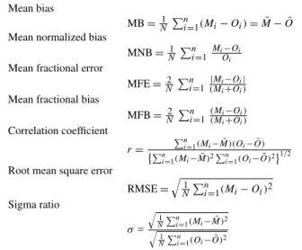
Table 3. Definition of the metrics used in the evaluation of the MOCAGE model performance.Mrefers to the model,Orefers to the observations.M¯ =_N1 P

(Mi) andO¯ =_N1 P(Oi).

Mean bias

MB=_N1 Pn_i₌₁(Mi−Oi)= ¯M− ¯O Mean normalized bias

MNB=_N1 Pn_i₌₁ Mi−Oi

Oi

Mean fractional error

MFE=_N2 Pn_i₌₁ |Mi−Oi|

(Mi+Oi)

Mean fractional bias

MFB=_N2 Pn_i₌₁ (Mi−Oi)

(Mi+Oi)

Correlation coefficient

r=

Pn

i=1(Mi− ¯M)(Oi− ¯O)

Pn

i=1(Mi− ¯M)2Pni=1(Oi− ¯O)2 1/2

Root mean square error

RMSE=

q 1 N

Pn

i=1(Mi−Oi)2 Sigma ratio σ= q 1 N Pn

i=1(Mi− ¯M)2

q 1 N

Pn

i=1(Oi− ¯O)2

study. The definitions of these metrics are indicated in Ta-ble 3. We also considered the mean diurnal cycle and the tem-poral series. Mean diurnal cycles are averaged over all avail-able days of concentrations for each 24 h period, while time series are based on the daily mean. Seasonal mean statistics are computed, with seasons corresponding to summer (June, July, August and September) and winter (December, January, February and March). We chose to study these two seasons of interest in air pollution while autumn and spring are rather transitional seasons. As summarized in Table 4, metrics are calculated for hourly values and daily averages for NOx, SO2

and PM10, while the hourly value and daily maximum 8-h

av-erage concentration (M×8h) statistics are computed for O3,

(5)

Table 4.Metrics considered in the evaluation of O3, NOx, SO2and PM10concentrations.

Indicators Parameters Codes

O3 NOx SO2 PM10

Mean bias hourly value MBO₃H MBNOxH MBSO2H –

daily mean – MBNOxDM MBSO2DM MBPM10

M×8h MBO₃MAX – – –

Mean normalized bias hourly value MNBO3H MNBNOxH MNBSO2H –

daily mean – MNBNOxDM MNBSO2DM –

M×8h MNBO3MAX – – –

Mean fractional bias daily mean – – – MFBPM10

Mean fractional error daily mean – – – MFEPM10

Correlation coefficient hourly value CORRO3H CORRNOxH CORRSO2H –

daily mean – CORRNOxDM CORRSO2DM CORRPM10

M×8h CORRO3MAX – – –

Roor mean square error hourly value RMSEO₃H RMSENOxH RMSESO2H –

daily mean – RMSENOxDM RMSESO2DM –

M×8h RMSEO3MAX – – –

Sigma ratio hourly value σO3H σNOxH σSO2H –

daily mean – σNOxDM σSO2DM σPM10

M×8h σO3MAX – – –

SOMO35* M×8h SOMO35 – – –

* SOMO35: annual sum of excess of daily maximum 8-h mean ozone over the cut-off of 35 ppb.

2.3 Observations and representativeness

In order to evaluate the performance of MOCAGE and to be in position to investigate and put into context the differ-ences between the simulations, we used AirBase (Version 5) measurement data. The AirBase metadata describes both the site area (urban, suburban or rural) and the site type (traf-fic, industrial or background). Giving the spatial resolution of our model (0.2◦×0.2◦), not all the reporting sites are rep-resentative enough. In Joly and Peuch (2012), an objective classification of the AirBase sites based on past measure-ments has been proposed in order to overcome issues of lack of homogeneity and erroneous information in the metadata. This classification allows for selection of the monitoring sites that are representative of the spatial resolution of our model. Through 10 classes, the less polluted stations (class 1) are distinguished from the very polluted sites (class 10). The ro-bustness of this approach is obtained with a pollutant-specific classification, taking into account that transport, chemistry and lifetime are specific to each pollutant.

In order to highlight the effect of site representativeness, we have compared the summertime (JJAS) average diurnal cycles for classes 1–2 (1 and 2), 1–5, 1–10 and 6–10 over France for O3and NOx(Fig. 1) for the simulation ANALY.

The median diurnal cycles observed (red) and simulated with MOCAGE (black) are presented for the year 2007. As shown in Fig. 1, the modeled variability of ozone and NOx is not

as pronounced as in observations, whatever the type of sites. During nighttime hours, ozone levels decrease when polluted stations are added to the sample (statistics for classes 1–2

a)O3 b)NOx

Fig. 1.Mean diurnal cycles of O₃(a)and NOx(b), as a function of

hour, simulated with MOCAGE (dashed lines) and observed by Air-Base (solid lines) averaged for the summer (JJAS) of 2007. Diurnal cycles are represented for the classes 1–2, 1–5, 1–10 and 6–10.

versus for classes 1–10) due to titration by NO. Nevertheless, simulated O3values do not decrease as much as the

observa-tions for classes 6–10 and 1–10. As expected, a large vari-ation in observed NOxconcentrations is seen when the

sta-tions considered are from different class types. Except when considering sites of classes 1–2, the amplitude of NOx

con-centrations is generally underestimated by the model. The amplitude of the median diurnal cycles changed significantly between categories 1–2 and 1–5 both for NOxand O3. For

classes 6–10 and 1–10, i.e. when most polluted sites are con-sidered, the model does not reproduce the high observed val-ues because, at least in part, of the model’s horizontal reso-lution.

(6)

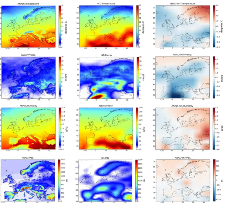
Fig. 2.From top to bottom: average summertime surface temperature (◦C), precipitation (mm d−1), humidity (g kg−1) and planetary bound-ary layer height (m) for the summer period (JJAS) of ANALY and INT. Differences between ANALY and INT are shown on the right.

improvement in accounting for representativeness. For NOx,

which are short lived species, it is necessary to reduce the sample of sites to classes 1–2 only to focus on sites that are representative enough for the model grid size. Due to transport effects, 5 classes (1–5) can be used to evaluate simulations for longer-lived species such as O3 in order to

have a larger geographical basis. The spatial distribution of PM10 (not shown) has the same behavior as O3, and the

same conclusion can be applied. In conclusion, the perfor-mances of MOCAGE will be assessed by comparing simula-tions against observasimula-tions at sites of classes 1–5 for O3and

PM10, and of classes 1–2 for NOxand SO2(not shown, but

same behavior as NOx). The number of sites finally taken

into account for each pollutant and country are summarized in Table 5.

3 Results

(7)

Table 5.Number of representative sites available by countries and species. Countries are, from left to right, France (FR), Spain (ES), England (GB), Germany (DE), Italy (IT) and Poland (PL).

Species Classes Countries

Europe FR ES GB DE IT PL

O3 1–5 970 201 191 33 202 54 47

NOx 1–2 354 68 115 – 97 9 –

SO2 1–2 342 31 101 7 101 17 7

PM10 1–5 824 168 151 47 259 – 28

CLIM, allow us to detect the effects due to the meteorolog-ical forcings and to changes in surface exchange fluxes, re-spectively. As described previously, ARPEGE analyses and ARPEGE-Climate fields differ regarding horizontal resolu-tion. Surface exchanges (emissions that depend upon me-teorology, as well as surface deposition) have been com-puted with two sets of meteorological conditions (ARPEGE and ARPEGE-Climate). The differences are for the biogenic volatile organic compounds, desert dust and sea salt emis-sions, as well as for deposition velocities, which depend on meteorology. Section 3.2 presents statistical skill scores of ANALY and CLIM against AirBase data (for “representative sites” only).

3.1 Comparisons between ANALY, INT and CLIM

3.1.1 Impact of changes in meteorological fields on European air pollution levels

Figure 2 shows the mean differences in surface temperature, precipitation, humidity and planetary boundary layer height (PBL) for the JJAS period between ANALY and INT run. The purpose is to evaluate briefly how climate meteorolog-ical forcings differ from the analyses. For the comparisons, we have thus averaged spatially the analyses fields to a hor-izontal resolution similar to the climate run. Focusing on the temperature first, similar structures are found over Eu-rope and an increasing gradient from the northern to the Mediterranean areas. However, over the northeastern part of the domain, the temperatures simulated by ANALY are locally significantly higher up to 4–5◦C. In contrast, over the Italian and Greek areas, INT displayed higher tempera-tures. The lower resolution of INT described previously ex-plains partly the differences observed because ANALY dis-plays more structured fields. Orography is smoothed in INT and the fields are representative of the current decade. Higher precipitations are simulated by INT over Europe and North Africa, but the spatial patterns are similar between the two simulations. Concerning the humidity, the spatial pattern is correctly reproduced by ARPEGE-Climate, with higher hu-midity over the Mediterranean Sea. The PBL is another im-portant field to be considered as it affects the dilution of pollutants in the atmosphere. As depicted in Fig. 2, higher

average PBLs in ANALY than in INT are seen over Spain and Greece.

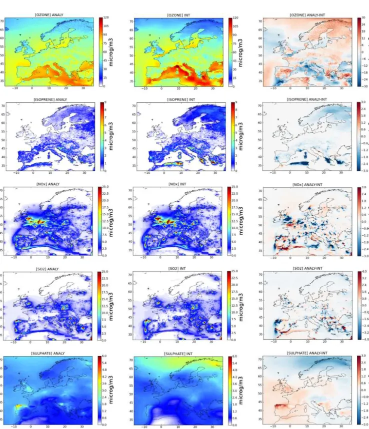
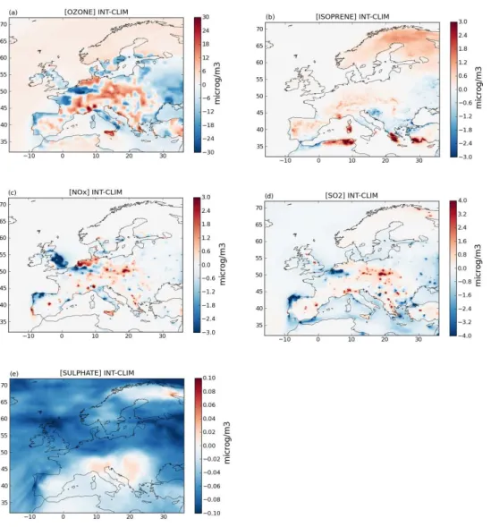
In Fig. 3, we represent the average surface concentra-tions of O3(a), isoprene (b), NOx(c), SO2(d) and sulphate

aerosols (e) for the summertime 2004–2008 in ANALY and INT. Here, the observed changes in pollutant distributions are only due to differences in the meteorological conditions, as emissions and deposition velocities are identical. The spatial pattern of mean O3concentrations is similar for the two

sim-ulations over the European domain. The highest concentra-tions are found in Southern Europe, over the Mediterranean Sea (50–60 ppbv), caused by intense photochemical produc-tion of O3(EEA, 2005; Vautard et al., 2005). The

meteoro-logical fields such as temperature influence the production of O3(Meleux et al., 2007; Hedegaard et al., 2008). Fields of

change in O3present some similarities to the changes in

tem-perature (Fig. 2). As noticed previously, over Spain, Africa and Northern Europe ANALY outputs higher temperatures up to 4–5◦C and higher O3concentrations (+6–8 ppbv). The

highest positive temperature differences seen over Europe relate to the highest positive O3 differences. Other studies

have shown that among all the meteorological parameters, the one that causes the greatest impact on ozone is temper-ature (Dawson et al., 2007). Nevertheless, as explained in Katragkou et al. (2010), other variables such as differences in solar radiation, zonal and meridional winds and changes in atmospheric stability also impact ozone concentrations. Similar temperatures and O3spatial patterns with the

oppo-site sign are observed over the Mediterranean basin (Italy, Greece).

High concentrations of isoprene, in the range of 2.5– 3 ppbv, are simulated over North Africa and Greece with the simulation INT. The biogenic emissions calculated to drive ANALY and INT are the same, but the differences in sim-ulated isoprene cannot be explained by the isoprene emis-sions or the temperature fields. A longitudinal cross-section (not shown) at a latitude of 36◦N (across Africa) displays higher isoprene concentrations at the surface from 0 to 10◦ with INT. The accumulation of isoprene near the surface can mainly be explained by the boundary layer, which is less well-mixed in INT than in ANALY.

The simulated distributions of summertime average NOx

concentrations (NO+NO2) show levels around 8–12 ppbv in

the Netherlands, Belgium, central and eastern England and the industrial Po Valley (Fig. 3). In ANALY and INT, higher concentrations of NOx are also found over major shipping

routes (North Sea, Gibraltar) and near emissions sources. Tropospheric columns of NOx(not shown) are identical in

ANALY and INT; the differences seen over Europe at the sur-face are mainly explained by differing boundary layer mixing in the two experiments.

Simulated SO2 concentrations over Europe display their

(8)

Fig. 3.From top to bottom: simulated average JJAS surface O3, isoprene, NOx, SO2and sulphate fields for ANALY and INT. Differences

(9)

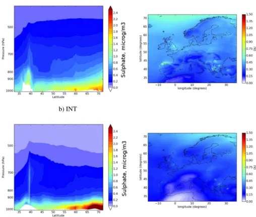
a) ANALY

b) INT

Fig. 4.On the left: latitudinal cross-sections at 30◦E of sulphate concentrations (µg m−3) averaged for the JJAS period. Levels are in hPa. On the right: sulphate column (DU) averaged for the summertime period of ANALY and INT.

Fig. 5. (a)Emissions of isoprene for the summertime period, averaged for 2004–2008 in the INT (left) and CLIM (middle) simulations.

(10)

Fig. 6.Differences in simulated average surface O3(a), isoprene(b), NOx(c), SO2(d), and sulphate(e)fields between INT and CLIM for

the summertime (JJAS). Species are in units of µg m−3.

(due to large plant sources in coastal Spain in the emissions dataset). Similar geographical distributions and ground lev-els of SO2 are observed in ANALY and INT. Once emitted

in the atmosphere, SO2 leads to the formation of sulphate

aerosols. Over the northeastern part of the domain, the lev-els of sulphate are higher in INT than in ANALY. Figure 2 shows higher precipitation and humidity in ANALY than in INT over this area. These differences imply enhanced trans-formation of SO2 into sulphate aerosols but also increased

wet deposition; those two contrasting effects can explain the differences seen in sulphate concentrations for the two simu-lations. Figure 4 represents a latitudinal cross-section of sul-phate at the longitude of 30◦E, averaged for the summertime period of 2004–2008 (JJAS). From 60◦N to 70◦N, the ver-tical extent of the sulphate distribution is lower in INT than in ANALY. The difference in sulphate near the surface is due to differing PBL mixing properties in the two simulations.

Tropospheric columns of sulphate (Fig. 4) indeed indicate very similar quantities in the two simulations.

To sum up, meteorological forcings (temperature, humid-ity, horizontal and vertical winds) differ in ANALY and INT. These differences lead to changes in the vertical and horizon-tal simulated distributions of pollutants. For all pollutants, primary as well as secondary, differences are primarily due to differing PBL mixing heights in the two simulations.

3.1.2 Impact of changes in surface exchanges on European air pollution levels

(11)

Fig. 7.O3deposition velocity averaged for the summertime period simulated by INT (left) and CLIM (middle). Differences between INT

and CLIM are shown on the right.

emissions in INT and CLIM are shown. Temperature and solar radiation are key driving variables that regulate emis-sions of isoprene and other biogenic volatil organic com-pounds (BVOCs) (Guenther et al., 1993, 1995, 2006). In accordance with the temperature field differences (Fig. 2), higher levels of isoprene are emitted in INT over central Spain, Central Europe, Scandinavia and the northeastern part of Africa than in CLIM. The changes in isoprene emissions induce corresponding changes in the geographical pattern of isoprene concentrations. Elevated concentrations of iso-prene (>1 ppbv) are observed over Central Europe, Greece and North Africa in INT compared to CLIM (Fig. 6b). The mean deposition fluxes (µg m−2s−1) of isoprene (Fig. 5b) show smaller differences between INT and CLIM.

Over Central Europe, O3deposition velocities are higher

by up to 0.2–0.3 cm s−1in INT than in CLIM (Fig. 7). Av-erage nighttime and daytime velocities have been calculated for both INT and CLIM; daytime is considered to be from 08:00 to 16:00 UTC and nighttime is considered to be from 20:00 to 04:00 UTC. For INT, daytime and nighttime mean deposition velocities reach 0.57 cm s−1and 0.24 cm s−1, re-spectively, over land (0.06 cm s−1and 0.05 cm s−1over sea). For CLIM, daytime and nighttime mean deposition velocities reach 0.54 cm s−1 _{and 0.24 cm s}−1 _{over land (0.05 cm s}−1

and 0.04 cm s−1_{over sea). Over land, similar deposition}

ve-locities are thus calculated in INT and CLIM. Higher veloci-ties are found during the day as it is known that O3deposition

velocity has a strong diurnal cycle due to increase in surface resistance at night. The mean deposition fluxes (µg m−2s−1) of O3, NOx, SO2and sulphate have been computed for the

summertime period (Fig. 8). In Fig. 6, the changes in concen-trations between INT and CLIM follow the changes in depo-sition fluxes and velocities. Where higher depodepo-sition fluxes are seen in INT than in CLIM (parts of Spain, England, Italy and the north and west of France), higher concentrations of ozone are simulated in CLIM. On the contrary, over other ar-eas (mainly in Central Europe) the mean deposition flux is higher in CLIM compared to INT, leading to higher concen-trations in INT than in CLIM.

In contrast with O3, smaller differences in flux deposition

are observed for NOx, SO2and sulphate; nevertheless, these

differences lead to differing concentrations between INT and CLIM. In the case of NOx, higher concentrations observed

in CLIM over the northern area (as in England, Belgium) are related to lower flux deposition at the surface. In addi-tion, SO2 concentrations rise by 1–1.5 ppbv in CLIM over

northern Spain and Belgium (Fig. 6c); the simulated changes are related to the SO2deposition fluxes (Fig. 8c). Very

simi-lar distribution and levels of sulphate aerosol are observed in INT and CLIM (Fig. 6e) across Europe.

In summary, the comparisons between ANALY and CLIM represented in Fig. 9 have revealed the contribution of both meteorological and flux changes to simulated air pollutants. The differences linked to the meteorological parameters or surface processes are pollutant dependent. Depending on the species that are considered, the differences can be driven mainly by the meteorological fields or the emission invento-ries. The meteorological and surface process effects can also compensate each other. Over the whole domain, the changes in sulphate concentrations between ANALY and CLIM are mostly determined by chemical, physical and dynamical pro-cesses due to the meteorological fields (humidity, precipita-tion). The major changes in isoprene concentrations (Spain, North Africa, Greece) are attributed to both changes in atmo-spheric circulation and stability (ANALY vs INT), as well as to differences in surface emissions and deposition (INT vs CLIM). For the short lived species NOxand SO2, we see that

the larger changes are localized near the high emission spots. In case of SO2, the differences between ANALY and CLIM

over Europe are explained by both the changes in deposition fluxes and by the meteorological fields. The O3concentration

differences between the two simulations are partly related to the changes in meteorological fields (such as temperature) but are principally due to the changes in deposition veloci-ties.

3.2 Statistical results: ANALY and CLIM against AirBase

(12)

Fig. 8.From top to bottom:(a)deposition flux of O3,(b)deposition flux of NOx,(c)deposition flux of SO2and(d)deposition flux of

sulphate. Deposition flux are in µg m−2s−1and averaged for the summertime period of INT and CLIM simulations.

the impacts of chronology of pollution events on the skill scores.

3.2.1 Model interannual variability

Figure 10 represents the temporal series of the model (ANALY in black line; CLIM in gray line) and monthly mea-sured AirBase data (red line) as an average of the daily mean O3 (a), NOx (b), SO2 (c) and particulate matter PM10 (d)

from 2004 to 2008 across the European domain. If we sub-tract the observed and simulated annual cycle averaged for the period 2004–2008 from these time series, positive and negative anomalies remain. The meteorology of ANALY is expected to follow the day-to-day variability in a more

realistic way than CLIM, which reproduces the climate of the decade 2000–2010. The interannual variability of O3

simu-lated by ANALY follows the measured variability of mete-orological events in terms of correlation and amplitude. The positive and negative anomalies estimated for ANALY are in-deed mostly correlated with the observations (CORRO3H=

0.61). This is obvious for the case of the summer 2006 heat wave. A positive anomaly, slightly underestimated, is cal-culated with ANALY, while this summer was particularly extreme with an intense production of O3(Struzewska and

Kaminski, 2008) compared to the mean level of the period 2004–2008. Table 6 summarizes the statistics of the hourly mean and daily M×8h O3 levels, averaged for the annual

(13)

Fig. 9.Same as Fig. 6 but comparing ANALY and CLIM.

stations considered (Table 5). If the annual trend and the interseasonal variability are reproduced, a systematic neg-ative bias is detected with CLIM throughout the summers (MBO3H= −4.6 µg m−3, MBO3MAX= −5.2 µg m−3).

The model–observation comparisons of NOxpresented in

Fig. 10b highlight a slightly overestimated annual ampli-tude of the concentrations for ANALY (with too high win-ter values and too low summer values), while the winwin-ter NOx values simulated by CLIM are much more

overesti-mated (MBNOxDM=8 µg m−3). The dynamics and the

in-tensities of the anomalies are often well-captured by the simulation ANALY; the positive anomalies estimated at the beginning of 2005 and 2006 are for instance well corre-lated with the observations. Winter pollution characterized by high levels of NOx (30–40 µg m−3) is depicted on the

time series. For ANALY, the statistics compiled in Table 7

show better performance in term of correlation in winter (CORRNOxH=0.42; CORRNOxDM=0.55) than in

sum-mer (CORRNOxH=0.29; CORRNOxDM=0.43). During

winter, chemical processes that lead to O3production are less

dominant compared to transport and could explain such dif-ferences (Bessagnet et al., 2004).

Time series of monthly mean concentrations of SO2from

the AirBase stations and the model simulations are repre-sented in Fig. 10c. Results show that the SO2

concentra-tions are overestimated for both ANALY and CLIM. Over-all, a good agreement is observed for the anomalies between ANALY and the observations in term of amplitude. From the year 2006, we notice a decrease in the observed SO2

(14)

a)O3 b)NOx

c)SO2 d)PM10

Fig. 10.(1) Simulated (ANALY: black lines; CLIM: gray lines) and measured (at the AirBase stations; red lines) time series of monthly mean concentrations of O3(a), NOx(b), SO2(c)and PM10(d). The time series are plotted from 1 January 2004 to 31 December 2008 and

averaged over the European domain. Concentrations are in µg m−3. (2) Anomalies calculated when subtracting the average annual series from the time series in (1).

Table 6.Seasonal and annual statistics obtained with MOCAGE over Europe at the AirBase stations. Statistics are averaged for the 5-yr period. Summer: June, July, August and September; winter: December, January, February and March. The calculated statistics are mean bias (MBO3H, MBO3MAX; µg m−3), mean normalized bias (MNBO3H, MNBO3MAX, %), correlation coefficient (CORRO3H,

CORRO3MAX), root mean square error (RMSEO3H, RMSEO3MAX; µg m−3) and sigma ratio (σH,σMAX). Statistics are computed for

the O₃hourly value and O₃M×8h. SOMO35 values are in µg m−3d.

O3metrics ANALY CLIM

Year JJAS DJFM Year JJAS DJFM MBO3H 2.7 −2.9 6.4 −5.3 −4.6 −8.2

MNBO3H 5.1 −4.5 13.8 −9.8 −7.7 −17.7

CORRO3H 0.61 0.59 0.58 0.3 0.32 0.17

RMSEO3H 24.7 24.9 24.3 34.3 35.4 34.1

σH 0.87 0.73 1.04 0.98 0.97 1.08

MBO3MAX 0.01 −8.1 5.7 −6.3 −5.2 −9.1

MNBO₃MAX 0.04 −9.44 9.8 −8.8 −5.9 −15.5 CORRO3MAX 0.7 0.63 0.65 0.4 0.04 0.25

RMSEO₃MAX 21.3 21.4 21.5 32.7 35.2 32.2

σMAX 0.85 0.66 1.09 0.99 0.90 1.22

(15)

Table 7.Same as Table 6 for hourly value and daily mean NOxconcentrations.

NOxmetrics ANALY CLIM

Year JJAS DJFM Year JJAS DJFM MBNOxH −0.19 −2.5 2.2 2.1 −2.1 8.4

MNBNOxH −1.2 −32.5 13.9 17.0 −28.8 55.1

CORRNOxH 0.46 0.29 0.42 0.14 0.08 0.05

RMSENOxH 13.2 8.8 15.9 20.5 10.6 29.2

σNOxH 1.20 0.91 1.19 1.64 1.00 1.78

MBNOxDM −0.12 −2.4 2.2 2.1 −2.1 8.0

MNBNOxDM −0.67 −32.4 14.6 17.5 −27.9 54.3

CORRNOxDM 0.61 0.43 0.55 0.20 0.09 0.07

RMSENOxDM 9.8 6.1 11.9 17.6 7.6 25.7

σNOxDM 1.34 0.98 1.30 1.92 1.07 2.08

Table 8.Same as Table 6 for hourly value and daily mean SO2concentrations.

SO2metrics ANALY CLIM

Year JJAS DJFM Year JJAS DJFM MBSO2H 0.39 −0.06 0.79 0.46 −0.06 1.3

MNBSO₂H 18.6 −2.9 36.7 24.2 −3.1 50.8 CORRSO2H 0.23 0.15 0.27 0.02 −0.01 −0.01

RMSESO₂H 4.3 3.3 4.9 5.5 3.8 7.4

σSO2H 1.37 1.16 1.53 1.65 1.21 2.05

MBSO₂DM 0.37 −0.07 0.79 0.45 −0.07 1.25 MBNSO2DM 17.8 −3.5 35.4 23.2 −4.0 49.7

CORRSO2DM 0.36 0.3 0.4 0.03 −0.01 −0.01

RMSESO2DM 3.2 2.3 3.7 4.5 2.8 6.29 σSO2DM 1.53 1.35 1.70 1.92 1.47 2.42

strategies in some European countries during the period of 2000–2010 (EEA, 2007). In our simulations, we kept the same emissions inventory representative of the year 2003. According to the time series of anomalies, and as described in Table 8, the biases calculated in ANALY and CLIM are of the same order of value (MBSO2DM=0.37 µg m−3 for

ANALY and MBSO2DM=0.45 µg m−3for CLIM).

Although the simulation ANALY presents a persistent negative bias (Table 9), it has the capability to reproduce the dynamics of PM10 for each year. The underestimation

of PM10 can be explained principally by the lack of

sec-ondary particulate and nitrate aerosols in our representa-tion of PM10. During summer, when photochemistry

fa-vors the formation of these particulates, the biases be-tween simulated and observed concentrations become greater (MBPM10DM= −11.9 µg m−3, Fig. 10 and Table 9). In the

case of CLIM, the time series of anomalies displays the capa-bility of the model to reproduce the particulate matter events (CORRPM10DM=0.39), although the model hardly

repro-duces their amplitude.

3.2.2 Statistical results

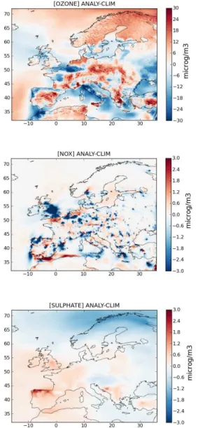
The statistics of the model are spatially displayed in Fig. 11; we illustrate the mean biases for O3daily M×8h values, as

well as for NOxand SO2daily mean concentrations across

the representative European stations. The scores are aver-aged for the summer season (JJAS). Regarding the results of simulation ANALY in the case of O3, two distinct spatial

regimes can be distinguished from the figures; positive and low biases are shown over Germany while negative biases are noticed in Spain and Italy. The correlations (not shown) are also more elevated in the northern part of Europe, no-tably in Germany (0.6–0.8) while in Southern Europe (Italy and Spain), the performance of the model is rather low (Pay et al., 2010). Comparisons between the statistical metrics of ANALY and CLIM indicate comparable biases over Eu-rope for the daily M×8h O3. The spatial distribution and

(16)

Table 9.Same as Table 6 for the PM10daily mean. The calculated statistics are MBPM10DM (µg m−3), MFBPM10DM (%), MFEPM10DM

(%), CORRPM10DM, RMSEPM10DM (µg m−3) andσPM10DM.

PM10metrics ANALY CLIM

Year JJAS DJFM Year JJAS DJFM MBPM₁₀DM −8.2 −11.9 −4.6 −5.3 −11.8 4.6 MFBPM10DM −59.5 −94.6 −33.6 −48.5 97.9 3.5

MFEPM10DM 75.1 96.9 58.0 85.4 101.7 77.4

CORRPM10DM 0.39 0.2 0.48 0.04 −0.04 0.03

RMSEPM10DM 15.1 14.4 15.1 21.6 15.3 28.3

σPM₁₀DM 0.96 0.49 1.02 1.39 0.60 1.59

a)O3 b)NOx c)SO2

Fig. 11.Spatial distribution of mean bias (µg m−3) for daily M×8h O3(a), daily mean NOx(b)and daily mean SO2(c)concentrations for

the average summertime period of 2004–2008. The two rows represent ANALY (top) and CLIM (bottom).

Table 6, for ANALY, annual correlations of hourly values and daily M×8h O3 concentrations reach 0.61 and 0.7,

re-spectively. Also, annual and seasonal MNB values for hourly and daily M×8h O3show good performance in accordance

with the recommendation of US-EPA (MNBE≤ ±15 %). In summer, the model tends to slightly underestimate the hourly levels of O3 (MBO3H= −2.9 µg m−3) and daily

M×8h concentrations (MBO3MAX= −8.1 µg m−3), while

it overestimates concentrations in winter months (MBO3H=

6.4 µg m−3_{; MBO}

3MAX=5.7 µg m−3). Correlation values

are lowest for both hourly values and daily M×8h over winter, 0.58 and 0.65, respectively. During winter, O3 is

controlled by processes other than photochemistry (such as boundary conditions, deposition, titration); O3 is thus

sen-sitive to physical and dynamic characteristics (higher reso-lution of forcings, emissions, deposition velocities). Higher

negative biases are thus exhibited by CLIM in wintertime (MBO3H= −8.2 µg m−3; MBO3MAX= −9.1 µg m−3), as

seen in Fig. 10, due to the differences in deposition ve-locities and in the concentrations in the lower atmosphere. Daily M×8h are also best reproduced by the model (corre-lations between 0.63 and 0.7); the variability of daily M×8h is mainly driven by photochemistry as well as the bound-ary layer height. To examine if the model is able to simulate the variability of O3concentrations, we used the sigma

(17)

considered: SOMO35 and the number of exceedance days. SOMO35 corresponds to the yearly sum of the differences between daily maximum 8 h running average concentrations that are greater than 35 ppb (Amann et al., 2005). It is used as an indicator for O3health impact and is recommended by the

World Health Organization (WHO). The values of SOMO35 are summarized in Table 6. When averaged over all of the European stations considered, the observed seasonal levels reach 2221 µg m−3d and 496 µg m−3d in summer and win-ter, respectively (4118 µg m−3d for the all year). Both sim-ulations catch the levels of SOMO35 and the seasonal vari-ation (van Loon et al., 2007). According to ANALY, about 40 % of the SOMO35 is produced during summer and 20 % during winter. Over the summer period, the number of days with O3 exceeding the 120 µg m−3 threshold for the daily

maximum 8-h average concentration is underestimated in ANALY (n=5.7 days) and fairly well estimated in CLIM (n=12 days), in comparison to the observations (n=15.4 days) from the European stations. The mean ozone concen-trations above the threshold of 120 µg m−3 for the M×8h simulated by ANALY are mostly in line with the observa-tions or within the interannual variability. More elevated val-ues are reached in CLIM than ANALY, as shown for the French and Italian stations (Fig. 12a). Figure 12b shows the percentile of daily O3maximum simulated by ANALY and

CLIM simulations. The interval between the 20th and 70th percentiles display similar values for both simulations. The occurrence of extreme values (maxima) is underestimated by the model for both simulations. As seen previously, above the threshold of 180 µg m−3_{, CLIM simulates a higher number of}

occurrences than the observations. These figures depict, how-ever, overall that MOCAGE driven by climate model outputs as forcings is able to simulate realistic ozone concentrations over Europe.

As exposed in Table 5, 354 stations were used to provide NOxmeasurements throughout Europe. Considering the

spa-tial distribution of mean biases for daily mean NOx,

statisti-cal results show satisfactory seasonal mean bias for ANALY (MBNOxDM= −2.4 µg m−3 during summer) without

spa-tial pattern between north and south. Similar geographical distributions and values of mean bias are displayed for CLIM (Fig. 11), while the summer mean bias reaches−2.1 µg m−3 (Table 7). The spatial distribution of the correlation coeffi-cients shows a large variability per station; while northern stations display high correlations (0.6< r <0.8), low corre-lations are observed in Southern Europe (r <0.4). The per-formances of the model are reduced with CLIM for all sea-sons, notably during winter (Fig. 7) when the concentrations of NOxare overestimated, as shown in Fig. 10. Thus, in

win-ter, MNBNOxH and MNBNOxDM reach 55.1 % and 54.3 %,

respectively; also, RMSENOxH and RMSENOxDM reach

29.2 µg m−3 and 25.7 µg m−3, respectively. In summer, the MNB values for hourly and daily mean are near the uncer-tainty proposed by EC and US-EPA for the ANALY simula-tion. Globally, the annual and seasonal daily mean statistics

a)

b)

Fig. 12. (a)Summertime average ozone concentrations (over the stations available) above the threshold of 120 µg m−3over 6 Eu-ropean countries. FR is France, ES is Spain, DE is germany, GB is England, IT is Italy, and PL is Poland. The standard deviation measuring the interannual variability is represented by the vertical bars.(b)Distribution of daily O3maximum percentiles for AirBase

measurements (red) and MOCAGE simulations (ANALY in black, CLIM in gray).

present better performances in comparison with the hourly values.

For SO2, low correlations are mainly concentrated in

Southern Europe (coefficients under 0.2), as in Spain, while some northern stations display high correlations (r >0.7) in regard to statistical results of ANALY. Averaged over all Eu-ropean stations, the summertime mean correlation of daily mean SO2reaches 0.3. Considering the mean bias for

sum-mer (Fig. 11), low biases are depicted across all the stations (MBSO2DM= −0.07 µg m−3for ANALY and CLIM).

Nev-ertheless, the stations located in Poland display high positive biases (>2 µg m−3). The uncertainties of the emissions in-ventory in Eastern Europe may contribute to the higher bias observed. In some stations in Spain, higher bias is also ob-served, due to the emission inventory in part. The regulation of SO2 emissions in Spain have lead to an emission

(18)

in Table 8, the highest correlations are obtained in winter (CORRSO2H=0.27; CORRSO2DM=0.40), but the

con-centrations are overestimated leading to a high value of MNB close to the EC criteria.

As seen in Fig. 10, the model presents a systematic negative bias for the simulated concentrations of PM10.

For the ANALY simulation, the correlation coefficient for the annual daily mean is 0.39, while it reaches 0.2 and 0.48 for the summer and winter season, respectively (Ta-ble 9). The spatial distribution of mean bias and correlations (not shown here) present a homogeneous pattern over Eu-rope. The annual MFE (MFEPM10DM=75.1 %) and MFB

(MFBPM10DM= −59.5 %) calculated for ANALY does not

meet the performance criteria or the performance goal pro-posed by Boylan and Russell (2006). The performance of the model is better during winter when the MBPM10DM is

about−4.6 µg m−3_(against _{−11.9 µg m}−3_{in summer) and}

the mean correlation reaches 0.48 (against 0.2 for the sum-mer). The underestimation of PM10can be explained by the

lack of secondary particulate and nitrate aerosols in our rep-resentation of PM10. Differences between the seasons are

linked to chemical processes, dominant in summer, which favor the formation of these particulates and increase the bias between simulated concentrations (lacking these chemi-cal processes) and observations.

Several air quality models operated in Europe have been evaluated either individually or in comparison to other mod-els in the literature. In the following discussion, a quick com-parison with other regional air quality models (Hass et al., 2003; van Loon et al., 2004, 2007) and MOCAGE will be carried out in order to situate our model among the com-munity. For this reason, we used the studies similar with our simulation ANALY, which had a long time scale of 1 yr over the European domain on a regional scale with hori-zontal resolutions similar to MOCAGE. Also, these mod-els were evaluated against ground observations at rural sites from AirBase and EMEP. Concerning O3 daily M×8h,

sat-isfactory performances are displayed with MOCAGE, in terms of annual MNB values: 0.04 % versus −1 to 10 %; correlations: 0.7 versus 0.69–0.84 (van Loon et al., 2007); and RMSE: 21.3 µg m−3versus 18.1–25.5 µg m−3(van Loon et al., 2004). Values for summer and winter daily M×8h O3

are also in the range of other models, as for the correlations (0.63 versus 0.61–0.77 for summer; 0.65 versus 0.45–0.62 for winter) and the MNB (−9.44 % versus−5 to 8 % for summer; 9.8 % versus−20 to 15 % for winter) according to the study of van Loon et al. (2007). The MOCAGE perfor-mances for NOx can be compared with the performance of

NO2in other models. The annual correlation of daily mean

NOxobtained in this study reaches 0.61, compared to 0.03–

0.52 (Hass et al., 2003; van Loon et al., 2004) and the RMSE value is around 9.8 µg m−3 versus 8.5–13.9 µg m−3 (Hass et al., 2003; van Loon et al., 2004). As for O3, the MOCAGE

results for SO2show good performances in comparison with

the other studies. The annual daily mean correlation is among

the higher values (0.36 versus 0.24–0.49). The calculated RMSE reaches 3.2 µg m−3 _{against 2.7–10.9 µg m}−3_{for the}

other models (Hass et al., 2003; van Loon et al., 2004). For PM10, statistical results are in the same range as for other

studies; nevertheless, the annual daily mean correlation is rather low and reaches 0.39 compared to 0.38–0.55; the an-nual RMSE is 15.1 µg m−3(versus 12.4–16.6 µg m−3).

To summarize, MOCAGE performs well according to the comparisons between ANALY and AirBase observations, as discussed previously. The statistical scores of O3, NOx and

SO2 display satisfactory performances compared to other

studies, while the accuracy in our representation of PM10

exhibits poorer results, which are expected by design. Com-parisons between the simulations ANALY and CLIM have shown that the geographical distribution of mean biases are quite similar for each pollutant considered. In this section, the model to observation comparisons were based on a com-mon approach, which consists in comparing each year of the simulation with the matching measured values from the Air-Base database. In CLIM, the meteorological forcings are rep-resentative of the current decade; there is no particular match in the sequence of years, and the representativeness of the skill scores can be assessed by permutations of all years. By doing the same for ANALY, the comparisons will allow us to determine which statistical tools are useful to consider for future studies.

3.2.3 Impacts of chronology of pollution events

We evaluated each year of the simulations with 5 yr of mea-surements, giving 25 model-to-date pairs of statistics for both ANALY and CLIM. On the time basis of the 2004–2008 pe-riod, we calculated every possible permutation, but on this period of 5 yr, we did not consider the same year of measure-ments more than once. We also filtered out the cases when one or more simulated years correspond with the same years of data. Finally, these conditions let us consider 44 realiza-tions, which provide a large statistical basis.

In order to give a concise statistical summary, we used the Taylor diagrams, which indicate how well observed and sim-ulated patterns match each other in terms of correlation and normalized standard deviation (NSD) (Taylor, 2001). The correlation coefficientR gives a measure of the co-variance of simulated and observed values. The NSD gives a mea-sure of the amplitude of the variance in modeled values ver-sus observed values. When NSD reaches a value lower than 1, it means that the temporal standard deviation in simu-lated values is lower than observed. Figure 13 shows the normalized Taylor plots that summarize the ANALY and CLIM permutations. The statistics are computed for the sum-mertime daily M×8h O3 concentrations (a) and daily

av-erages of NOx (b) and SO2 (c). For each plot, “ANALY”

(19)

Fig. 13.Taylor plots of the comparison between modeled and observed M×8h O3concentrations, daily mean NOxand daily mean SO2. The

radial distance from the origin corresponds to NSD, andRcorresponds to the azimuthal position.

Table 10.Seasonal JJAS statistics obtained with the permutations ANALY-p and CLIM-p. Statistics are the median values of the per-mutations. The calculated statistics are mean bias (µg m−3), mean normalized bias (%), correlation coefficient, root mean square error (µg m−3) and sigma ratio. Statistics are computed for the O3hourly

value and daily M×8h concentrations.

O₃metrics

ANALY-p CLIM-p ANALY MBO₃MAX −7.9 −5.6 −8.1 MNBO3MAX −9.1 −6.4 −9.4

CORRO3MAX 0.04 0.07 0.63

RMSEO3MAX 31 34.6 21.4

σO3MAX 0.67 0.9 0.66

MBO3H −2.8 −5.0 −2.9

MNBO3H −4.4 −7.9 −4.5

CORRO3H 0.33 0.34 0.59

RMSEO3H 30.9 35.1 24.9

σO₃H 0.75 0.98 0.73

the results of ozone first, comparisons between ANALY and ANALY-p confirm there is no day-to-day variability with the permutations of ANALY-p as shown by the correlations. As summarized in Table 10, for ANALY-p, the median value of the correlations reach 0.04 (against 0.63 for ANALY). The median RMSE of ANALY-p are not as good as the me-dian RMSE for ANALY for both the hourly (RMSEO3H=

31 µg m−3_{for ANALY-p and 21.4 µg m}−3_{for ANALY) and}

daily M×8h (RMSEO3MAX=30.9 µg m−3 for ANALY-p

and 24.9 µg m−3_{for ANALY) of O}

3. Nevertheless, very

sim-ilar values of MNBO3MAX and MNBO3H in the ranges of

−9 % and−4.5 %, respectively, are obtained. The standard deviation values (σ) are similar in ANALY and ANALY-p and range around 0.66, meaning that the model underesti-mates the daily M×8h ozone variability. The same conclu-sions can be extended to the daily averages of NOx, SO2

(Table 11) and PM10 (Table 12) concentrations. ANALY

and ANALY-p only differ by the correlations while the MB, RMSE and variances are quite similar. For the daily mean NOx(Fig. 13), the NSD are close to the reference, meaning

that the amplitude of the simulated NOxagrees with the

(20)

Table 11.Same as Table 10 for hourly values and daily average of NOxand SO2.

NOxmetrics SO2Metrics

ANALY-p CLIM-p ANALY ANALY-p CLIM-p ANALY MBNOxDM −2.5 −2.0 −2.4 MBSO2DM −0.09 −0.04 −0.07

MNBNOxDM −32.6 −27.8 −32.4 MNBSO2DM −2.8 −1.0 −3.5

CORRNOxDM 0.09 0.07 0.43 CORRSO2DM −0.004 0.005 0.3

RMSENOxDM 7.1 7.6 6.1 RMSESO2DM 2.6 2.7 2.3

σNOxDM 0.98 1.07 0.98 σSO2DM 1.39 1.47 1.35

MBNOxH −2.5 −2.1 −2.5 MBSO2H −0.08 −0.04 −0.06

MNBNOxH −32.7 −28.6 −32.5 MNBSO2H −2.6 −0.68 −2.9

CORRNOxH 0.09 0.07 0.29 CORRSO2H −0.008 −0.01 0.15

RMSENOxH 9.9 10.5 8.8 RMSESO2H 3.6 3.8 3.3

σNOxH 0.90 0.98 0.91 σSO2H 1.18 1.21 1.16

Table 12.Seasonal JJAS statistics obtained with the permutations ANALY-p and CLIM-p. Statistics represent the median values of the permutations. The calculated statistics are mean bias (µg m−3), mean fractional bias (%), mean fractional error (%), correlation co-efficient, root mean square error (µg m−3) and sigma ratio. Statis-tics are computed for the PM10daily mean concentrations.

PM₁₀metrics

ANALY-p CLIM-p ANALY MBPM10DM −11.9 −11.8 −11.9

MFBPM10DM −93.8 −98.6 −94.6

MFEPM10DM 97 102.2 96.9

CORRPM10DM 0.01 0.01 0.2

RMSEPM10DM 14.9 15.1 14.4

σPM₁₀DM 0.49 0.59 0.49

than ANALY due to the permutations. The RMSE values increase by 19 %, 11 % and 8 % for the hourly values of O3, NOxand SO2, respectively, from ANALY to

ANALY-p. However, for the metrics MB, MNB andσ, similar values are computed.

For O3 (Fig. 13), low and similar correlations of daily

M×8h levels are calculated for both ANALY-p and CLIM-p. As shown in Table 10, the correlations between the observed and simulated hourly values (0.33 for ANALY-p and 0.34 for CLIM-p) are higher than daily M×8h. The daily vari-ability of ozone, characterized by higher levels during after-noon and lower values during nighttime hours is still cap-tured with the permutations. The RMSE values show lower performances for CLIM-p compared to ANALY-p for both daily M×8h (+10 %) and hourly O3 (+13 %) levels. The σ values indicate the tendency of ANALY-p to underesti-mate ozone variance in summer. The CLIM-p simulations show better σ values (0.9 and 0.98 versus 0.67 and 0.75 for ANALY-p), which is unexpected and cannot be inter-preted as greater performance. The MNB of M×8h ozone

show a tendency of model underestimation as the median reaches−9.1 % in ANALY-p and −6.4 % in CLIM-p. For the hourly and daily average NOxand SO2concentrations,

the simulations ANALY-p and CLIM-p are now well corre-lated (Table 11). During summer, ANALY-p and CLIM-p un-derestimate the daily mean and hourly NOxconcentrations.

From ANALY-p to CLIM-p, the median MNBNOxDM and

MNBNOxH change by about 14 % while the RMSENOxDM

and RMSENOxH change by about 7 %. Concerning the

am-plitude of the NOxvariances (Fig. 13), a satisfactory

agree-ment is observed;σ reaches 0.98 in ANALY-p and 1.07 in CLIM-p for daily mean NOx(Table 11). For the SO2results,

the variance is overestimated by the model for both ANALY-p and CLIM-ANALY-p. For the daily mean of PM10concentrations,

the amplitude of the variances are in line for ANALY-p and CLIM-p simulations. The simulations underestimate the variability of the PM10 (σPM10DM=0.49 for ANALY-p

andσPM10DM=0.59 for CLIM-p). MBPM10DM reaches

similar values for ANALY-p and CLIM-p. MFB and MFE metrics do not reach the performance criterion.

To summarize, the use of permutations have made the comparisons between the simulations suitable for discussion of the statistical results. Comparisons between the reference case “ANALY” with “ANALY-p” corroborate the incorrect phasing between the measurements and simulations when the day-to-day variability is not reproduced. Finally, the results allow us to conclude that statistical metrics such as variances, MB, MNB and RMSE give robust and sound information when climate forcings are used to drive the model.

4 Conclusions

(21)

qualify and properly interpret statistical conclusions that can be drawn from simulations of air quality in a future climate.

The comparisons between three 5-yr experiments allow us to quantify the relative importance of changes in surface fields and upper air meteorology. We find that both elements contribute to changes in O3 concentrations. Differences in

sulphate aerosols and in isoprene (as a proxy for biogenic volatile organic compounds) are mainly related to changes in meteorology and mixing, while it is the contrary for SO2

and NOx, which essentially depend upon changes in surface

fluxes.

The skill of the reference simulation (analysed forcings) to reproduce European surface observations is in the range of previous reference evaluation studies (Hass et al., 2003; van Loon et al., 2004, 2007). As expected, the simulation based upon forcings from a climate model is not as skillful at repro-ducing observations, since it cannot follow day-to-day varia-tions by design. Nevertheless, the geographical distribuvaria-tions of the mean biases are similar in the two simulations. The comparisons of SOMO35 and the distribution of O3

maxi-mum percentiles support the capability of MOCAGE, driven by meteorological fields from a climate model, to simulate realistic European ozone levels.

The objective of this work was to determine useful sta-tistical metrics that can be used for models driven by climate model meteorological parameters. For O3, we show that

sim-ulations using either analyses or climate model forcings fol-low the same tendency: hourly and M×8h concentrations are slightly underestimated and the biases and RMSE are in the same range of values. Similar conclusions are observed for the daily averaged and hourly values of NOx and SO2, as

well as daily PM10. The amplitude of variance is accurately

reproduced when the model is driven by climate fields. Fi-nally, as for the standard deviation, statistical results of MB, MNB and RMSE can be interpreted with some degree of con-fidence.

Supplementary material related to this article is available online at: http://www.geosci-model-dev.net/5/ 1565/2012/gmd-5-1565-2012-supplement.pdf.

Acknowledgements. This work was partly founded by ADEME

(Agence De l’Environnement et de la Maitrise de l’Energie, http://www.ademe.fr). We would like to thank N. Poisson (ADEME), L. Rouil (INERIS) and M. Beekman (CNRS/LISA) for useful discussions.

Edited by: P. J¨ockel

The publication of this article is financed by CNRS-INSU.

References

Amann, M., Bertok, I., Cofala, J., Gyarfas, F., Heyes, C., Klimont, Z., Schopp, W., and Winiwater, W.: Clean air for Eu-rope (CAFE) programme final report, Tech. rep., 2005. Andersson, C. and Engardt, M.: European ozone in a future climate:

Importance of changes in dry deposition and isoprene emissions, J. Geophys. Res., 115, D02303, doi:10.1029/2008JD011690, 2010.

Bechtold, P., Bazile, E., Guichard, F., Mascart, P., and Richard, E.: A mass-flux convection scheme for regional and global models, Q. J. Roy. Meteor. Soc., 127, 869–886, 2001.

Bessagnet, B., Hodzic, A., Vautard, R., Beekmann, M., Cheinet, S., Honor´e, C., Liousse, C., and Rou¨ıl, L.: Aerosol modeling with CHIMERE-preliminary evaluation at the continental scale, At-mos. Environ., 38, 2803–2817, 2004.

Bousserez, N., Atti´e, J.-L., Peuch, V.-H., Michou, M., Pfis-ter, G., Edwards, D., Emmons, L., Mari, C., Barret, B., Arnold, S. R., Heckel, A., Richter, A., Schlager, H., Lewis, A., Avery, M., Sachse, G., Browell, E. V., and Hair, J. W.: Eval-uation of the MOCAGE chemistry transport model during the ICARTT/ITOP experiment, J. Geophys. Res., 112, D10S42, doi:10.1029/2006JD007595, 2007.

Boylan, J. and Russell, A.: PM and light extinction model perfor-mance metrics, goals, and criteria for three-dimensional air qual-ity models, Atmos. Environ., 40, 4946–4959, 2006.

Carvalho, A., Monteiro, A., Solman, S., Miranda, A., and Bor-rego, C.: Climate-driven changes in air quality over Europe by the end of the 21st century, with special reference to Portugal, in: Environmental Science and Policy, Elsevier, Oxford, England, 445–558, 2010.

Chang, J. and Hanna, S.: Air quality model performance evaluation, Meteor. Atmos. Phys., 87, 167–196, 2004.

Courtier, P., Freydier, C., Geleyn, J. F., Rabier, F., and Rochas, M.: The ARPEGE project at M´et´eo France, in: Atmospheric Models, vol. 2, Workshop on Numerical Methods, Reading, UK, 193– 231, 1991.

Cuvelier, C., Thunis, P., Vautard, R., Amann, M., Bessagnet, B., Bedogni, M., Berkowicz, R., Brandt, J., Brocheton, F., Built-jes, P., Coppalle, A., Denby, B., Douros, G., Graf, A., Hell-muth, O., Honor´e, C., Hodzic, A., Jonson, J., Kerschbaumer, A., de Leeuw, F., Minguzzi, E., Moussiopoulos, N., Pertot, C., Pirovano, G., Rou¨ıl, L., Schaap, M., Stern, R., Tarrason, L., Vig-nati, E., Volta, M., White, L., Wind, P., and Zuber, A.: CityDelta: a model intercomparison study to explore the impact of emis-sion reductions in European cities in 2010, Atmos. Environ., 41, 189–207, 2007.