Universidade$Federal$de$São$Carlos$
Centro$de$Ciências$Biológicas$e$da$Saúde$
Programa$de$Pós@graduação$em$Ecologia$e$Recursos$Naturais$
G
USTAVO(H
ENRIQUE(DE(C
ARVALHO(
RELAÇÕES$ENTRE$AMBIENTE,$TRAÇOS,$COMPOSIÇÃO$E$
FUNCIONAMENTO$DE$COMUNIDADES$VEGETAIS$DE$
CERRADO$
Orientador:$Dr.$Marco$Antônio$Batalha$
Universidade$Federal$de$São$Carlos$
Centro$de$Ciências$Biológicas$e$da$Saúde$
Programa$de$Pós@graduação$em$Ecologia$e$Recursos$Naturais$
G
USTAVO$H
ENRIQUE$DE$C
ARVALHO$
RELAÇÕES$ENTRE$AMBIENTE,$TRAÇOS,$COMPOSIÇÃO$E$
FUNCIONAMENTO$DE$COMUNIDADES$VEGETAIS$DE$
CERRADO$
Ficha catalográfica elaborada pelo DePT da Biblioteca Comunitária/UFSCar
C331ra
Carvalho, Gustavo Henrique de.
Relações entre ambiente, traços, composição e funcionamento de comunidades vegetais de cerrado / Gustavo Henrique de Carvalho. -- São Carlos : UFSCar, 2013.
151 f.
Tese (Doutorado) -- Universidade Federal de São Carlos, 2013.
1. Cerrados. 2. Comunidades vegetais. 3. Funcionamento de comunidades. 4. Modelos de equações estruturais. I. Título.
Dedico'aos'meus'pais,'Jerônimo'e'Sueli,'e'à'minha'noiva,'
AGRADECIMENTOS$
Agradeço$ao$Prof.$Dr.$Marco$Antônio$Batalha,$pela$sempre$pronta$disponibilidade$e$
orientação.$Aos$meus$pais,$por$terem$me$dado$os$meios$para$chegar$até$aqui.$Ao$
CNPq,$CAPES$e$FAPESP$pelas$bolsas$e$auxílios$financeiros.$À$direção$do$Parque$
Nacional$das$Emas,$pela$licença$concedida.$Aos$companheiros$de$laboratório,$pela$
ajuda$nos$trabalhos$de$campo$e$amizade.$Finalmente,$à$minha$noiva,$Cláudia,$por$ter$
SUMÁRIO$
Abstract$...$7$
Resumo$...$8$
Introdução$geral$...$9$
Capítulo$1$...$20$
Summary$...$22$
Introduction$...$24$
SEM$Software$...$27$
Model$specification$...$28$
Model$identification$...$33$
Checking$data$requirements$...$34$
Model$estimation,$fit,$interpretation,$and$modification$...$37$
Conclusion$...$43$
References$...$43$
Capítulo$2$...$57$
Summary$...$59$
Introduction$...$61$
Materials$and$methods$...$64$
Results$...$69$
Discussion$...$71$
Abstract$...$95$
Introduction$...$96$
Materials$and$methods$...$99$
Results$...$106$
Discussion$...$108$
References$...$112$
Capítulo$4$...$131$
Abstract$...$133$
Introduction$...$134$
Materials$and$methods$...$135$
Results$...$137$
Discussion$...$138$
References$...$140$
ABSTRACT$
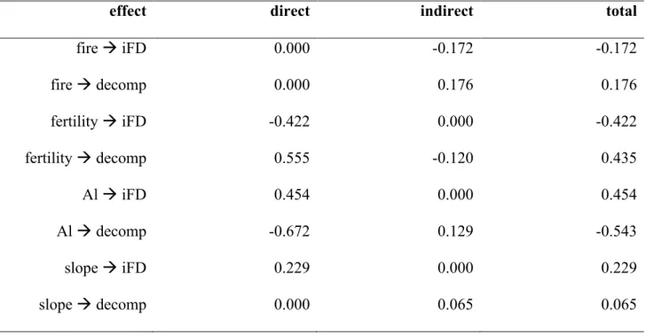
Understanding$how$biodiversity$and$ecosystem$functioning$will$respond$to$changes$in$the$ environment$is$fundamental$to$avoid$the$loss$of$species$and$ecosystem$function.$In$realistic$ scenarios,$ the$ biodiversity6ecosystem$ functioning$ pathway$ may$ account$ for$ only$ a$ small$ share$of$all$factors$determining$ecosystem$function.$.$In$the$last$chapter,$we$described$how$ the$ use$ of$ latent$ variables$ and$ structural$ equation$ models$ could$ be$ a$ useful$ tool$ for$ environmental$ research.$ In$ the$ second$ chapter,$ we$ investigated$ the$ strength$ to$ which$ variations$ in$ environmental$ characteristics$ in$ a$ Neotropical$ savanna$ affected$ functional$ diversity$ and$ litter$ decomposition.$ We$ sought$ an$ integrative$ approach,$ using$ structural$ equation$modelling$to$connect$fire$frequency,$soil$fertility,$exchangeable$aluminium,$water$ availability,$functional$diversity$of$woody$plants,$and$litter$decomposition$rates$in$a$causal$ chain.$By$expressing$these$hypotheses$simultaneously,$we$revealed$a$number$of$direct$and$ interactions.$We$found$significant$effects$of$soil$nutrients,$water$availability,$and$aluminium$ on$functional$diversity$and$litter$decomposition.$Fire$did$not$have$a$significant$direct$effect$ on$ functional$ diversity$ or$ litter$ decomposition.$ However,$ fire$ was$ connected$ to$ both$ variables$ through$ soil$ fertility.$ In$ the$ third$ chapter,$ we$ tested$ if$ we$ could$ predict$ local$ abundances$ using$ a$ pool$ of$ species$ and$ traits.$ To$ test$ if$ traits$ improved$ the$ predictions$ generated$ by$ the$ information$ present$ in$ the$ pool,$ we$ used$ maximum$ entropy$ models$ coupled$ with$ permutation$ tests.$ We$ could$ accurately$ predict$ local$ abundances$ of$ the$ 73$ species$in$the$pool.$Dispersal$limitation$was$the$main$factor$assembling$communities$at$all$ the$ scales$ we$ studied,$ but$ the$ importance$ of$ stochasticity$ increased$ in$ local$ scales.$ Traits$ explained$ little$ of$ the$ uncertainty$ present$ in$ local$ abundances,$ but$ coupled$ with$ pool$ frequencies$ they$ yielded$ large$ coefficients$ of$ determination.$ In$ the$ fourth$ chapter,$ we$ showed$how$fire$and$soil$fertility$influence$different$sets$of$traits$in$different$ways,$which,$in$ turn,$influence$community$composition$and$density.$
Keywords:$ cerrado,$ community$ assembly,$ community$ functioning,$ structural$ equation$
RESUMO$
Entender$ como$ a$ biodiversidade$ e$ o$ funcionamento$ dos$ ecosistemas$ vão$ responder$ às$ mudanças$ nas$ condições$ ambientais$ é$ essencial$ para$ a$ manutenção$ das$ interações$ que$ influenciam$as$propriedades$dos$ecossistemas.$Os$sistemas$ecológicos$respondem$à$mudanças$ nas$condições$ambientais$não$apenas$por$meio$da$interação$direta$com$essas$condições,$mas$ também$ de$ maneira$ indireta,$ via$ organismos.$ No$ primeiro$ capítulo,$ descrevemos$ o$ uso$ de$ variáveis$ latentes$ e$ modelos$ de$ equações$ estruturais$ em$ ecologia.$No$ segundo$ capítulo,$ nós$ investigamos$ como$ variações$ em$ características$ ambientais$ resultam$ em$ variações$ na$ diversidade$funcional$e$funcionamento$de$uma$comunidade$de$arbustos$e$árvores$de$cerrado$ no$ Parque$ Nacional$ das$ Emas$ (GO).$ Nós$ usamos$ modelagem$ de$ equações$ estruturais$ para$ quantificar$os$efeitos$da$fertilidade$do$solo,$alumínio,$disponibilidade$de$água$e$diversidade$ funcional$na$decomposição$de$serapilheira.$Nós$encontramos$efeitos$diretos$entre$nutrientes$ do$ solo,$ disponibilidade$ de$ água$ e$ alumínio$ na$ diversidade$ funcional$ e$ funcionamento$ da$ comunidade.$O$fogo$não$teve$um$efeito$direto,$mas$sim$caminhos$indiretos$pelos$quais$o$fogo$ influencia$ a$ diversidade$ funcional$ e$ o$ funcionamento.$ No$ terceiro$ capítulo,$ nós$ procuramos$ identificar$ a$ importância$ de$ processos$ determinísticos$ e$ estocásticos$ na$ composicão$ da$ comunidade$ vegetal$ do$ cerrado$ em$ Emas.$ Nós$ testamos,$ por$ meio$ de$ modelos$ de$ máxima$ entropia$e$testes$de$permutação,$se$os$traços$das$espécies$adicionariam$informação$relevante$ para$a$previsão$das$abundâncias$além$da$informação$já$presente$no$repositório$de$espécies.$ Nossos$modelos$tiveram$alto$poder$de$previsão$para$as$73$espécies$do$repositório.$Limitação$ de$ dispersão$ foi$ o$ principal$ processor$ compondo$ as$ comunidades.$ Processos$ estocásticos$ também$tiveram$grande$importância,$principalmente$na$escala$local.$Sem$a$informação$prévia$ sobre$as$frequências$das$espécies,$modelos$com$os$traços$tiveram$pouco$poder$de$explicação.$ Entretanto,$ ao$ combinarmos$ traços$ e$ frequências$ no$ repositório,$ nossos$ modelos$ resultaram$ em$ altos$ coeficientes$ de$ determinação.$ No$ último$ capítulo,$ nós$ mostramos$ como$ fogo$ e$ fertilidade$do$solo$influenciam$diferentes$grupos$de$traços$e$como$esses$traços$influenciam$na$ composição$e$densidade$das$comunidades.$$
INTRODUÇÃO$GERAL$
Prever$ como$ a$ biodiversidade$ e$ o$ funcionamento$ dos$ ecossistemas$ responderão$ às$ mudanças$ nas$ condições$ ambientais$ é$ essencial$ para$ a$ manutenção$ das$ propriedades$ dos$ ecossistemas$ e$ dos$ serviços$ que$ eles$ provêm$ (Loreau$et' al.$ 2001).$ Em$ comunidades$ vegetais,$ tal$ entendimento$ pode$ levar$ à$ políticas$ de$ conservação$ mais$ efetivas,$ especialmente$ aquelas$ que$ referem6se$ ao$ manejo$ de$ agentes$ de$ perturbação,$ como$ o$ fogo,$ para$ minimizar$ a$ perda$ de$ espécies$ e$ serviços.$ Vários$ estudos$ tiveram$ como$ objetivo$investigar$as$interações$entre$fatores$abióticos,$diversidade$biológica$ e$ funcionamento$ dos$ ecossistemas$ (Tilman$et' al.$ 1997;$ Hooper$et' al.$ 2005).$ Entretanto,$ a$ maioria$ desses$ estudos$ analisou$ as$ relações$ entre$ apenas$ dois$ dos$ componentes$ mencionados,$ desconsiderando,$ principalmente,$ a$ influência$ de$ variações$ do$ ambiente$ na$ interação$ entre$ biodiversidade$ e$ funcionamento$dos$ecossistemas$(Tilman$et'al.$1997;$Hooper$&$Vitousek$1997;$ Hector$et'al.$1999).$
Os$ sistemas$ ecológicos$ respondem$ às$ mudanças$ nas$ condições$ ambientais$ não$apenas$por$meio$de$interação$direta,$mas$também$de$maneira$indireta,$ via$ organismos$ (Chapin$et' al.'1997;$ Cardinale$et' al.$ 2000).$ Dessa$ forma,$ ao$ considerarmos$as$relações$diretas$e$indiretas$entre$ambiente,$biodiversidade$ e$funcionamento,$teremos$dado$um$importante$passo$rumo$à$identificação$e$ quantificação$das$vias$que,$ultimamente,$influenciam$nas$propriedades$dos$ ecossistemas$(Srivastava$&$Vellend$2005).$A$investigação$das$interações$entre$ organismos$e$funcionamento$em$condições$ambientais$flutuantes$é$uma$das$ questões$ da$ ecologia$ de$ ecossistemas$ que$ necessita$ de$ mais$ atenção$$ (Srivastava$&$Vellend$2005).$
grupos$ de$ teorias$ procuram$ explicar$ o$ processo$ de$ formação$ de$ comunidades$à$partir$de$um$repositório$de$espécies$(Chase$et'al.$2005):$o$da$ teoria$ neutra,$ segundo$ a$ qual$ fatores$ aleatórios$ governam$ a$ formação$ de$ comunidades,$ uma$ vez$ que$ todas$ as$ espécies$ do$ repositório$ regional$ são$ funcionalmente$equivalentes,$ou$seja,$sneutrass$(Hubbell$2005,$2006)$e$o$das$ teorias$ baseadas$ nos$ nichos$ das$ espécies,$ segundo$ as$ quais$ fatores$ determinísticos$ são$ os$ principais$ responsáveis$ pela$ composição$ das$ comunidades$(Weiher$et'al.$1998).$
Nos$ modelos$ de$ formação$ de$ comunidades$ baseados$ em$ nichos,$ vários$ mecanismos$ de$ exclusão$ de$ espécies$ foram$ propostos.$ Um$ desses$ mecanismos$é$dos$filtros$ambientais,$segundo$o$qual$fatores$abióticos$como$$ fertilidade$ do$ solo$ e$ fogo$ determinam$ que$ espécies$ possuem$ as$ características$ necessárias$ para$ sobreviverem$ em$ um$ determinado$ local$ (Keddy$ 1992).$ De$ maneira$ semelhante,$ o$ processo$ de$ limitação$ da$ similaridade$ de$ nichos,$ causada$ principalmente$ pela$ interação$ entre$ as$ espécies$de$uma$comunidade,$também$deixa$uma$marca$nas$comunidades.$ Por$exemplo,$espécies$com$atributos$semelhantes$têm$mais$chance$de$terem$ alta$sobreposição$de$nichos,$o$que$faz$com$que$elas$tenham$que$competir$por$ recursos$(Fridley$2001;$Kraft$et'al.$2008;$Cornwell$&$Ackerly$2009).$Porém,$a$ competição$ por$ recursos$ faz$ com$ que$ as$ espécies$ limitem$ sua$ similaridade$ para$que$tenham$menor$sobreposição$de$nichos,$atuando$em$direção$oposta$ aos$filtros$ambientais.$
procurado$ por$ outras$ formas$ de$ medir$ a$ diversidade$ das$ comunidades$ e$ melhor$entender$como$os$organismos$respondem$ao$ambiente$e$influenciam$ no$ funcionamento$ dos$ ecossistemas$ (Petchey$ &$ Gaston$ 2002;$ Pavoine$et' al.$ 2011).$Uma$maneira$alternativa$de$se$medir$a$biodiversidade$é$olhando$para$ a$ diversidade$ de$ traços$ funcionais$ de$ uma$ comunidade.$ Foi$ sugerido$ que$ comunidades$ com$ maior$ diversidade$ de$ traços$ funcionais$ operam$ de$ maneira$mais$eficiente$devido$à$maior$complementaridade$de$nichos,$o$que$ leva$ ao$ particionamento$ de$ recursos$ (Díaz$ &$ Cabido$ 2001;$ Hooper$et' al.$ 2005).$ Ainda,$ a$ diversidade$ funcional$ pode$ abordar$ diferentes$ facetas$ do$ funcionamento$das$comunidades,$uma$vez$que$é$medida$por$meio$de$vários$ traços$funcionais$das$espécies$(Cadotte$2011).$Petchey$&$Gaston$(2002,$2006)$ propuseram$ um$ índice$ de$ diversidade$ funcional$ (FD)$ que$ estima$ a$ complementaridade$ de$ traços$ funcionais$ em$ comunidades.$ Maiores$ diferenças$ nos$ traços$ indicam$ maior$ complementaridade.$ Posteriormente,$ uma$ extensão$ do$ índice$ para$ levar$ em$ conta$ a$ variação$ intraespecífica$ foi$ proposta$(Cianciaruso$et'al.$2009).$
et'al.$2006;$Stokes$&$Archer$2010).$A$identificação$dos$processos$por$trás$da$ formação$ das$ comunidades$ é$ uma$ das$ questões$ centrais$ da$ ecologia$ (Sutherland$et'al.$2013).$
No$cerrado,$a$fertilidade$do$solo,$baixo$pH,$altas$concentrações$de$alumínio$e$ incidência$ de$ queimadas$ se$ apresentam$ como$ possível$ fatores$ ambientais$ que$ limitam$ a$ ocorrência$ de$ espécies.$ Dessa$ forma,$ filtros$ ambientais$ provavelmente$governam$a$ocorrência$de$plantas$em$áreas$de$cerrado.$Por$ exemplo,$ é$ notável$ a$ variação$ na$ densidade$ de$ plantas$ na$ vegetação$ do$ cerrado,$ indo$ desde$ fisionomias$ campestres,$ mais$ abertas,$ até$ fisionomias$ mais$fechadas,$com$alta$densidade$de$indivíduos$arbóreos.$Teorias$clássicas$$ sugeriram$que$o$cerrado$é$um$gradiente$de$fertilidade.$Assim,$a$densidade$ de$indivíduos$acompanharia$a$fertilidade$do$solo$(Goodland$&$Pollard$1973).$ Estudos$ recentes$ tanto$ corroboraram$ (Amorim$ &$ Batalha$ 2008;$ Silva$ &$ Batalha$2008),$quanto$não$corroboraram$(Ruggiero$et'al.$2002)$essas$teorias.$ Além$do$solo,$o$fogo$tem$sido$indicado$como$fator$ambiental$que$influencia$ a$ diversidade$ fenotípica$ (Batalha$ et' al.' 2011;$ Cianciaruso$ et' al.$ 2012)$ e$ filogenética$ (Silva$ &$ Batalha$ 2010;$ Cianciaruso$et' al.$ 2012)$ da$ vegetação$ do$ cerrado.$
diferentes,$ contribuindo$ para$ a$ importância$ do$ parque$ nos$ estudos$ de$ formação$e$funcionamento$de$comunidades$vegetais.$
No$primeiro$capítulo$da$tese,$nós$investigamos$os$papéis$direto$e$indireto$do$ fogo$ e$ do$ solo$ na$ diversidade$ funcional$ e$ funcionamento$ de$ uma$ comunidade$de$espécies$arbóreas$de$cerrado$no$Parque$Nacional$das$Emas.$ Nós$ buscamos$ uma$ abordagem$ integrada,$ quantificando$ todas$ as$ relações,$ diretas$ e$ indiretas,$ entre$ os$ fatores$ abióticos,$ bióticos$ e$ funcionamento.$ Assim,$ propusemos$ um$ modelo$ de$ equações$ estruturais$ com$ uma$ representação$plausível$de$como$as$variáveis$de$interesse$se$relacionam.$ No$segundo$capítulo$da$tese,$utilizamos$modelos$de$máxima$entropia$para$ prever$ a$ abundância$ das$ espécies$ arbóreas$ de$ cerrado$ no$ Parque$ Nacional$ das$ Emas$ por$ meio$ de$ alguns$ de$ seus$ traços$ funcionais.$ Fazendo$ isso,$ pudemos$particionar$a$importância$de$processos$determinísticos$e$aleatórios$ formação$ dessas$ comunidades.$ Ainda$ nesse$ capítulo,$ determinamos$ quais$ foram$ os$ traços$ mais$ contribuiram$ para$ as$ previsões,$ indicando,$ assim,$ aqueles$traços$que$mais$influenciam$as$abundâncias.$
No$ terceiro$ capítulo,$ procuramos$ explicar$ a$ riqueza$ e$ a$ densidade$ de$ indivíduos$arbóreos$no$Parque$Nacional$das$Emas$por$meio$da$relação$entre$ traços$ fisiológicos$ e$ de$ resposta$ e$ o$ histórico$ de$ fogo$ e$ disponibilidade$ de$ nutrientes$no$solo.$
Finalmente,$ no$ quarto$ capítulo,$ descrevemos$ o$ uso$ da$ modelagem$ de$ equações$ estruturais$ nas$ ciências$ ambientais,$ focando$ no$ uso$ de$ variáveis$ latentes,$ ainda$ pouco$ utilizadas.$ Procuramos$ apresentar$ os$ conceitos$ mais$ importantes$ da$ técnica,$ suas$ premissas,$ como$ estimar$ parâmetros$ e$ interpretar$os$resultados.$
$
REFERÊNCIAS$BIBLIOGRÁFICAS$
Amorim,$P.K.$&$Batalha,$M.A.$(2007)$Soil6vegetation$relationships$in$hyperseasonal$ cerrado,$seasonal$cerrado,$and$wet$grasslands$in$Emas$National$Park$(central$ Brazil).$Acta'Oecologica,$32,$3196327.$
Batalha,$ M.A.,$ Silva,$ I.A.,$ Cianciaruso,$ M.V.,$ França,$ H.$ &$ Carvalho,$ G.H.$ (2011)$ Phylogeny,$ traits,$ environment,$ and$ space$ in$ cerrado$ plant$ communities$ at$ Emas$National$Park$(Brazil).$Flora,$206,$9496956.$
Cadotte,$M.W.$(2011)$The$new$diversity:$management$gains$through$insights$into$ the$functional$diversity$of$communities.$Journal' of' Applied' Ecology,$48,$10676 1069.$
Cardinale,$ B.J.,$ Nelson,$ K.$ &$ Palmer,$ M.A.$ (2000)$ Linking$ species$ diversity$ to$ the$ functioning$ of$ ecosystems:$ on$ the$ importance$ of$ environmental$ context.$ Oikos,$91,$1756183.$
Chapin,$F.S.,$III.,$Walker,$B.W.,$Hobbs,$R.J.,$Hooper,$D.U.,$Lawton,$J.H.,$Sala,$O.E.$&$ Tilman,$D.$(1997)$Biotic$control$over$the$functioning$of$ecosystems.' Science,$ 277,$5006504.$
Chase,$J.M.$(2005)$Towards$a$really$unified$theory$for$metacommunities.$Functional' Ecology,$19,$1826186.$
Cianciaruso,$ M.V.,$ Batalha,$ M.A.,$ Gaston,$ K.J.$ &$ Petchey,$ O.L.$ (2009)$ Including$ intraspecific$variability$in$functional$diversity.$Ecology,$90,$81689.$
Cianciaruso,$M.V.,$Silva,$I.A.,$Batalha,$M.A.,$Gaston,$K.J.$&$Petchey,$O.L.$(2012)$The$ role$ of$ fire$ on$ phylogenetic$ and$ functional$ structure$ of$ woody$ savannas:$ moving$ from$ species$ to$ individuals.$Perspectives' in' Plant' Ecology,' Evolution' and'Systematics,$14,$2056216.$
Cornwell,$ W.K.$ &$ Ackerly,$ D.D.$ (2009).$ Community$ assembly$ and$ shifts$ in$ plant$ trait$ distributions$ across$ an$ environmental$ gradient$ in$ coastal$ California.$ Ecological'Monographs,$79,$1096126.$
Díaz,$S.$&$Cabido,$M.$(2001)"Vive"la"différence:"plant"functional"diversity"matters"to" ecosystem$processes.$Trends'in'Ecology'&'Evolution,$16,$6466655.$
Fridley,$ J.D.$ (2001)$ The$ influence$ of$ species$ diversity$ on$ ecosystem$ productivity:$ how,$where,$and$why?$Oikos,$93,$5146523.$
Goodland,$ R.$ &$ Pollard,$ R.$ (1973)$ The$ Brazilian$ cerrado$ vegetation:$ a$ fertility$ gradient.$Journal'of'Ecology,$61,$2196224.$
Gravel,$ D.,$ Canham,$ C.D.,$ Beaudet,$ M.,$ Messier,$ C.$ (2006)$ Reconciling$ niche$ and$ neutrality:$the$continuum$hypothesis.$Ecology'Letters,$9,$3996409.$
Hooper,$ D.U.,$ Chapin,$ F.S.III.,$ Ewel,$ A.H.,$ Hector,$ A.,$ Inchausti,$ P.,$ Lavorel,$ S.,$ Lawton,$ J.H.,$ Lodge,$ D.M.,$ Loreau,$ M.,$ Naeem,$ S.,$ Schmid,$ B.,$ Setälä,$ H.,$ Symstad,$ A.J.,$ Vandermeer,$ J.$ &$ Wardle,$ D.A.$ (2005)$ Effects$ of$ biodiversity$ on$ ecosystem$ functioning:$ a$ consensus$ of$ current$ knowledge.$ Ecological' Monographs,$75,$3635.$
Hooper,$D.U.$&$Vitousek,$P.M.$(1997)$The$effects$of$plant$composition$and$diversity$ on$ecosystem$processes.$Science,$277,$130261305.$
Keddy,$ P.A.$ (1992)$ Assembly$ and$ response$ rules:$ two$ goals$ for$ predictive$ community$ecology.$Journal'of'Vegetation'Science,$3,$1576164.$
Kraft,$N.J.B.,$Valencia,$R.$&$Ackerly,$D.D.$(2008)$Functional$traits$and$niche6based$ tree$community$assembly$in$an$Amazonian$forest.$Science,$322,$5806582.$ Laughlin,$ D.C.,$ Joshi,$ C.,$ van$ Bodegom,$ P.M.,$ Bastow$ &$ Fulé,$ P.Z.$ (2012)$ A$
predictive$model$of$community$assembly$that$incorporates$intraspecific$trait$ variation.$Ecology'Letters,$15,$129161299.$
Loreau,$ M.$ (2000)$ Biodiversity$ and$ ecosystem$ functioning:$ recent$ theoretical$ advances.$Oikos,$91,$3617.$
(2001)$ Biodiversity$ and$ ecosystem$ functioning:$ current$ knowledge$ and$ future$challenges.$Science,$294,$8046808.$
Macarthur,$ R.$ &$ Levins,$ R.$ (1967)$ The$ limiting$ similarity,$ convergence,$ and$ divergence$of$coexisting$species.$The'American'Naturalist,$101,$3776385.$
Mayfield,$M.$&$Levine,$J.M.$(2010)$Opposing$effects$of$competitive$exclusion$on$the$ phylogenetic$structure$of$communities.$Ecology'Letters,$13,$108561093.$
Pavoine,$S.,$Vela,$E.,$Gachet,$S.,$Bélair,$G.$&$Bonsall,$M.B.$(2011)$Linking$patterns$in$ phylogeny,$ traits,$ abiotic$ variables$ and$ space:$ a$ novel$ approach$ to$ linking$ environmental$filtering$and$plant$community$assembly.$Journal'of'Ecology,$99,$ 1656175.$
Petchey,$O.L.$&$Gaston,$K.J.$(2002)$Functional$diversity$(FD),$species$richness$and$ community$composition.$Ecology'Letters,$5,$4026411.$
Petchey,$O.L.$&$Gaston,$K.J.$(2006)$Functional$diversity:$back$to$basics$and$looking$ forward.$Ecology'Letters,$9,$7416758.$
Ruggiero,$P.G.C.,$Batalha,$M.A.,$Pivello,$V.R.$&$Meirelles,$S.T.$(2002)$Soil6vegetation$ relationships$ in$ cerrado$ (Brazilian$ savanna)$ and$ semideciduous$ forest,$ Southeastern$Brazil.$Plant'Ecology,$160,$1616.$
Shipley,$B.,$Paine,$C.E.T.$&$Baraloto,$C.$(2012)$Quantifying$the$importance$of$local$ niche6based$ and$ stochastic$ processes$ to$ tropical$ tree$ community$ assembly.$ Ecology,$93,$7606769.$$
Silva,$D.M.$&$Batalha,$M.A.$(2008)$Soil–vegetation$relationships$in$cerrados$under$ different$fire$frequencies.$Plant'and'Soil,$311,$87–96.$
Silva,$ I.A.$ &$ Batalha,$ M.A.$ (2010)$ Woody$ plant$ species$ co6occurrence$ in$ Brazilian$ savannas$under$different$fire$frequencies.$Acta'Oecologica,$36,$85691.$
Srivastava,$D.S$&$Vellend,$M.$(2005)$Biodiversity6ecosystem$functioning$research:$is$ it$ relevant$ to$ conservation?$ Annual' Review' of' Ecology,' Evolution,' and' Systematics,$36,$2676294.$
Sutherland,$ W.J.,$ Freckleton,$ R.P.,$ Godfray,$ H.C.J.,$ Beissinger,$ S.R.,$ Benton,$ T.,$ Cameron,$D.,$Carmel,$Y.,$Coomes,$D.A.,$Coulson,$T.,$Emmerson,$M.C.,$Hails,$ R.S.,$ Hays,$ G.C.,$ Hodgson,$ D.J.,$ Hutchings,$ M.J.,$ Johnson,$ D.,$ Jones,$ J.P.G.,$ Keeling,$ M.J.,$ Kokko,$ H.,$ Kunin,$ W.E.,$ Lambin,$ X.,$ Lewis,$ O.T.,$ Malhi,$ Y.,$ Mieszkowska,$ N.,$ Milner6Gulland,$ E.J.,$ Norris,$ K.,$ Phillimore,$ A.B.,$ Purves,$ D.W.,$Reid,$J.M.,$Reuman,$D.C.,$Thompson,$K.,$Travis,$J.M.J.,$Turnbull,$L.A.,$ Wardle,$ D.A.$ &$ Wiegand,$ T.$ (2013)$ Identification$ of$ 100$ fundamental$ ecological$questions.$Journal'of'Ecology,$101,$58667.$
Tilman,$D.$(2004)$Niche$tradeoffs,$neutrality,$and$community$structure:$A$stochastic$ theory$ of$ resource$ competition,$ invasion,$ and$ community$ assembly.$ Proceedings'of'the'National'Academy'of'Sciences,$101,$10854610861.$
Tilman,$ D.,$ Lehman,$ C.L.$ &$ Thomson,$ K.T.$ (1997)$ Plant$ diversity$ and$ ecosystem$ productivity:$theoretical$considerations.$Proceedings'of'the'National'Academy'of' Sciences'of'the'United'States'of'America,$94,$185761861.$
II$6$CAPÍTULO$1$
Basics of structural equation modelling in
1Ecology
2Running title: Structural equation modelling in Ecology
3Gustavo H. Carvalho
1*, Marco A. Batalha
1, and Owen L. Petchey
2 41
Plant Ecology Laboratory, Department of Botany, Federal University of São Carlos, PO Box 5
676, São Carlos, 13565-905, SP, Brazil. 6
2
Institute of Evolutionary Biology and Environmental Studies, University of Zurich, 7
Winterthurerstrasse 190, CH-8057, Zurich, Switzerland. 8
*
Summary
1The statistical methods ecologists commonly use to analyse their data are often unsuitable for 2
testing hypotheses were variables could act as cause and effect. Also, most of these methods do 3
not take into account the multidimensionality of some common concepts in ecology, such as 4
biodiversity and body size. Structural equation modelling (SEM) provides the means to 5
quantitatively test hypotheses that represent alternative causal structures of any level of 6
complexity. SEM allows researchers to analyse their data from a system perspective, with less 7
emphasis on bivariate relationships and more focus on the system of interacting variables. 8
Theoretical variables, such as biodiversity, are included in structural models as latent variables. 9
Latent variables cannot be directly measured, but arise from the variance shared by a set of 10
observed variables called indicators. Latent variable modelling also takes into account our 11
imperfections in taking measurements and the effects of variables not included in our models on 12
those included. These are modelled as error variances and measurement error in SEM and help 13
on building more faithful mathematical translations of our hypotheses. SEM, thus, yields a 14
powerful tool for gleaning knowledge on ecological theories, but requires a lot of attention from 15
users to render trustworthy results. From model specification to fit, passing through data 16
collection and screening, the researcher using SEM has to mind a number of assumptions. In this 17
article, we explain the basic concepts and assumptions of SEM analysing worked data, focusing 18
on avoidance of the common pitfalls. When used with the required caution, SEM is a powerful 19
set of tools that can be used to generate models about the functioning of a system and, ultimately, 20
reproduce, corroborate, and fine-tune these frameworks to generalise our knowledge and 21
Key-words: structural equation modeling, latent variable analysis, path analysis, causal 1
Introduction
1Ecologists commonly use standard univariate (for example, ANOVA, regression, GLMs) and 2
multivariate (such as principal component analysis, cluster analysis, and canonical 3
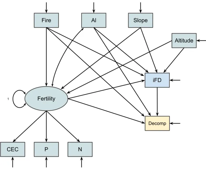
correspondence analysis) methods to analyse their data. These methods are often unsuitable for 4
testing hypotheses in which a variable can act as cause and effect, and hypotheses about chains 5
and networks of causation (Fig. 1). Furthermore, standard methods usually give estimators of net 6
effects instead of causal relationships and cannot accommodate theoretical ideas that are not 7
directly measurable (Kline 2010). Structural equation modelling (SEM), in contrast, provides the 8
means to quantitatively test hypotheses that represent alternative causal structures, be them 9
simple, with only a handful of variables, or more complex, with several variables, some of which 10
being both causes and effects. The hypotheses that can be tested via SEM are often described 11
using diagrams that describe the causal assumptions of the researcher regarding a set of variables 12
(Fig. 1). SEM allows researchers to look at their data from a systems perspective, with less 13
emphasis on bivariate relationships and more focus on the system of interacting variables (Kline 14
2010). 15
Sewall Wright proposed the first type of SEM in the beginning of the 20th century 16
(Wright 1918, 1921, 1937). At that time, Pearson’s school of statistics and correlation 17
dominated: causation was seen as a useless concept (Shipley 2000). Critics of Wright’s proposal 18
thought he was trying to infer causation from correlations (Niles 1922). Wright, however, was 19
trying to estimate the strength of associations between variables in a system that may include 20
causal knowledge and beliefs (Wright 1921). A few years later, Sir Ronald Fisher developed 21
methods for inferring causation based on randomisation and experimental control (Fisher 1925). 22
SEM has recently gained popularity, especially in the social sciences where it is now well 1
established. In ecology and evolution, SEM is less established, even though studies show its 2
efficacy for gleaning knowledge about the prior causal relationship assumed to result in observed 3
data. It has been used to analyse causes of, for example, plant species richness (Grace & Pugesek 4
1997), plant species succession (Vile et al. 2006), the abundance of rabbits and track numbers of 5
Iberian lynx and Egyptian mongoose (Palomares et al. 1998), and the overnight survival of house 6
sparrows (Pugesek & Tomer 1996). Furthermore, several books and papers provide excellent 7
guides to the philosophy, principles, and methods involved with SEM (Grace 2006, Kline 2010, 8
Schumacker & Lomax 2004, Shipley 2000). 9
Unfortunately, SEM can be complex and has numerous pitfalls. Possible source of 10
problems go from not respecting the underlying assumptions of the method to failure to properly 11
report results. Some of the common pitfalls have serious impacts on the validity and 12
reproducibility of the analyses. Here we provide an overview to the basic concepts of SEM, 13
focused on avoidance of the common and likely pitfalls. This overview we illustrate with 14
reference to a worked example, with data and complete R code available as a supplement. We 15
regularly indicate sources of the more in depth topics that we cannot cover. 16
Overview of the method
17SEM emphasises estimating the strengths of causal effects between variables through path 18
coefficients (Grace et al. 2010). A deeper discussion about causation can be found in Shipley 19
(2000), where he suggests that the common adage that ‘correlation does not imply causation’ 20
should be revised to ‘correlation implies an unknown causative structure’. Pearl (2000) further 21
technique of causal diagrams for testing causal assumptions from correlations. Here we use the 1
term ‘causal assumptions’ as a reference to all the prior knowledge a researcher has about certain 2
phenomena. Accordingly, we use ‘causal effects’ or simply ‘effects’ as the strength of such 3
causal assumptions. The purpose of SEM is not to establish cause from association. Instead, it 4
provides ways of statistically testing the strength of support for causal assumptions. 5
The first step in SEM is model specification: formulation of a hypothesis about the causal 6
relationships among the variables of interest (for instance, Fig. 1), with each causal relationship 7
representing a plausible ecological process. The variables might be directly observable or 8
unmeasured theoretical variables (see below). Similarly to more standard analyses, hypotheses 9
are ideally created before data collection. The second step in SEM is model identification, 10
whereby one examines if the specified model can be solved. The third step is checking the 11
requirements of the observed data, including examination of sample size, distribution, 12
collinearity, and outliers in and among variables. The fourth step is estimation of model (= 13
hypothesis) fit and parameter values. Model fit informs about how well the proposed model 14
explains the observed data and can be used to assess the support among a set of causal structures. 15
Parameter values indicate how much response variables change with changes in explanatory 16
variables. 17
Throughout this article, we focus on maximum likelihood estimation (MLE) to estimate 18
parameter values and maximum likelihood chi-squared (MLχ2) to assess model fit. Used this 19
way, SEM gives estimates of how well the models proposed explain the observed relationships 20
among variables, of the direct and indirect effects of one variable on another, and of how much 21
If models are not specified in advance, SEM can assist in data exploring by searching for 1
a causal structure (model) that best explains the data. The usual dangers associated with 2
exploratory analyses apply and interpretations of data produced by exploratory SEM should be 3
tested using new, independent data (Schumacker & Lomax 2004). 4
SEM Software
5A number of statistical software packages are capable of implementing structural equation 6
models. Some of the most popular packages include LISREL (Jöreskog & Sörbom 2006), EQS 7
(Bentler 1995), Mplus (Muthén & Muthén 1998-2010), R (R Development Core Team 2012), 8
and SPSS Amos (Arbuckle 1995-2009). The software is quite user-friendly and can analyse 9
models of varying complexity using different techniques to assess model fit and to estimate 10
parameters (Schumacker & Lomax 2004). The R environment for statistical analysis provides a 11
few choices of SEM package. OpenMX (Boker et al. 2011) is one of the most actively 12
developed. It has fewer parameter estimators than commercial packages, but is perfectly capable 13
in most usage scenarios and can be expanded to include more estimators. Other SEM packages 14
for R include sem (Fox et al. 2012) and lavaan (Rosseel 2012). lavaan is quite new, but already 15
offers several different types of estimation methods and is, feature-wise, on a par with 16
commercial packages. It also has useful supporting functions, including bootstrapping and 17
simulation of data, and is one of the easiest to use. The package sem has fewer features, but was 18
the first package to offer SEM support for R and was recently rewritten. Due to the popularity of 19
R, we have chosen it and the lavaan package to present a step-by-step guide to performing 20
for R has a few published datasets that can be used alongside lavaan and is a good starting point 1
for those who wish to learn SEM in R. 2
Model specification
3Specification of the structural part of an structural equation model 4
Translating previous knowledge, theories, ideas, and hypotheses into a causal structure to be 5
tested using SEM is probably the most difficult part of using the method. The researcher can do 6
this translation by starting with variables and then identifying hypotheses, theories, or processes 7
that might connect them. This initial step is greatly aided by drawing the causal structure in a 8
graphical representation (Fig. 1). In such a drawing, arrows (hypothetical causal effects) connect 9
variables (shapes) to give a causal structure to the model. Variables in rectangles are termed 10
observed variables because they are directly measurable. For instance, Shannon diversity 11
(shannon rectangle), and nitrogen content (nitrogen rectangle) are observed variables because 12
they are directly measurable. A structural equation model may contain only directly measurable 13
variables. Grace (2006) argues that path analysis (structural equation model with only directly 14
measurable variables) considers only one level of the theory being tested, the relationships 15
between the components of interest, as they do not account for error variances and variables that 16
cannot be directly measured (i.e., latent variables). Thus, latent variables add a powerful 17
dimension to structural equation models. 18
Biodiversity can be represented as a latent variable, for example, since it is a 19
multidimensional concept that cannot be reduced to a single value (Purvis & Hector 2000). 20
Concepts that are not directly measurable (latent variables, constructs or factors) are graphically 21
latent variables cannot be measured, we use other variables as their indicators or proxies. Each 1
indicator variable can be seen as a dimension of a multidimensional concept. In Fig. 1, 2
biodiversity has three indicators: shannon, which corresponds to Shannon’s diversity index 3
values; FD, a functional diversity index (Cianciaruso et al. 2009); and phylodiversity, a 4
phylogenetic diversity index (Allen et al. 2009). Each of these indicators represents a different 5
facet of biological diversity. Shannon diversity takes into account the identity and proportions of 6
the species in a given sample, FD accounts for the trait variation among individuals, and 7
phylodiversity is a measure of the phylogenetic diversity in a community. The two other latent 8
variables in Fig. 1, soil fertility and community functioning, each have indicators that correspond 9
to aspects of the hypothesised construct. 10
After drawing the causal network, some variables will have arrows only going out 11
(termed an exogenous variable, e.g., soil fertility in Fig. 1), some will have arrows going in and 12
some will have arrows going in an out of them. The latter two are termed endogenous variables 13
(e.g., biodiversity and community functioning in Fig. 1). 14
Any two variables can be directly (e.g., soil fertility and biodiversity in Fig. 1) or 15
indirectly connected (soil fertility and community functioning through biodiversity). Variables 16
are sometimes both directly and indirectly connected (soil fertility and community functioning). 17
Variables only indirectly linked are fully mediated whereas variables with both direct and 18
indirect causal paths are partially mediated. The absence of causal links between two variables is 19
a very strong assumption. When causally connected, the path linking two variables is usually free 20
to take on any value during estimation. However, if two variables are not causally connected, the 21
researcher imposes a fixed path coefficient of zero. This will lead to a predicted bivariate 22
Incorrectly translating previous knowledge into a model may lead to rejection of the 1
proposed model due to its poor fit. In SEM, making as few as one parameter fixed or free can 2
cause drastic changes in fit. The directionality of the paths is equally influential. Models where 3
all variables are only at one end of a causal chain (for instance, ! →!→!) are called recursive. 4
Models where a given causal chain can have the same variable at its both ends (for instance, 5
! →!→! →!) are called nonrecursive. Nonrecursive models often arise from uncertainty 6
about directionality leading to inclusion of bi-directional causality or covariances between 7
endogenous variables. Nonrecursive models require special attention and tend to be problematic, 8
so they are best avoided unless the nonrecursiveness is strongly backed by theory, which is 9
seldom the case. 10
Careful translation of theory and previous knowledge into a structural equation model at 11
this step is crucial since everything following assume that the model is correct (Kline 2010). 12
Sometimes the knowledge driving the specification of a model provides room for alternative 13
causal structures. This can be accommodated with the specification of competing models or with 14
a list of possible modifications of the causal paths to improve model fit later on. It is important to 15
come up with competing equivalent models at this point to make sure that theory and not an 16
exploratory search for the model with the best fit is driving specification. In cases where 17
exploratory latent variable analysis is indeed the aim of the researcher, he or she must make the 18
rationale behind this choice very clear. 19
Finally, more often than not data will already have been collected before model 20
specification and identification. In this situation, the researcher has to be extra careful and 21
propose models that are consistent with theory instead of trying to arrange the variables in a way 22
yet plausible model to use as example. Thus, it is not our intention to thoroughly test theories 1
regarding causal links between the environment, biological diversity, and community 2
functioning. A very detailed discussion on the specification of ecological structural equation 3
models can be found in Grace et al. (2010). Shipley (2000) and Grace (2006) also address this 4
topic in great detail. 5
Specifying the measurement part of structural equation model 6
The measurement model consists of the latent variables and their indicators (Fig. 2). Indicators of 7
latent variables are also known as manifest variables. The arrows pointing from a latent variable 8
to its indicators are termed loadings. This terminology arises from the idea that the immeasurable 9
latent variable loads or manifests itself on the indicators, thus causing them. 10
A latent variable arises from the variance shared by its indicators. Take, for example, the 11
measurement model in Fig. 2a. The grey area in Fig. 2b represents the latent variable in Fig. 2a. 12
Variance not shared by indicators (unshaded areas in Fig. 2b) does not go into the definition of 13
the latent variable. This unique variability, which is represented by the Greek letter epsilon (ε, 14
Fig. 1, 2, and 4), is referred to as measurement error. Measurement error may represent random 15
error and imprecisions during data collection and also the effects of omitted variables that have 16
some effect on the indicators. The same omitted variable can affect multiple indicators, making 17
error terms correlated. Researchers can include this correlation by linking variables with two-18
headed arrows (δ1, δ2, and δ3 in Fig. 2). Explicitly thinking about and modelling these error terms 19
provides SEM a very important advantage over other methods. 20
Latent variables also have error terms. For exogenous latent variables (e.g., soil fertility 21
in Fig. 1), they are called variance and are represented by a two-headed arrow beginning and 22
influence of all the omitted variables, much like the error of an indicator. Error associated with 1
an endogenous latent variable (biodiversity and community functioning in Fig. 1) is termed 2
disturbance and is the amount of factor variance not explained by the model. Disturbances often 3
are represented by the letter D (Fig. 1 and 2a). 4
Take, for instance, the latent variable biodiversity in Fig. 1. It is well acknowledged that 5
there is no single number that serves as a perfect measure of the biological diversity of a sample 6
(Purvis & Hector 2000). Instead, ecologists rely on several indices to represent the 7
multidimensionality of this concept. So, we used three indices as indicators of biodiversity, each 8
representing a dimension. The values we get for the indices cannot be fully explained by the 9
latent variable though. This unaccounted indicator variance is known as measurement error in 10
SEM jargon. As an example, an index of phylogenetic diversity does not perfectly explain the 11
phylogenetic relationships between the species of a community. These method imperfections 12
(e.g, poorly resolved phylogenies) are modelled as measurement error in SEM. 13
Careful consideration of measurement error and of the distinction between latent and 14
observed variables may contribute to the refinement and maturation of ecological theories. 15
Instead of including biodiversity as a latent variable, we might have included only Shannon 16
diversity. This would have resulted in loss of information about the multidimensionality of the 17
concept of biodiversity, and loss of information about our imprecisions in measuring this 18
concept. Both losses would result in a less realistic mathematical translation of current theory. 19
Since we assume indicators to be caused by the latent variable, all bivariate correlations 20
between indicators are expected to be somewhat high. Indicators with too little or too much 21
shared variance are likely to be improper and ought to be reconsidered. The number of indicators 22
three indicators are more prone to problems during identification and estimation. When possible, 1
structural equation models should include at least three indicators for each latent variable. If a 2
latent variable has only one indicator, the error variance of the single indicator is not modelled. 3
Unless the error variance is pre-set due to previous knowledge, measurement error is not 4
considered. Finally, contrarily to manifest variables, latent variables do not have scales. To set a 5
scale to a latent variable, the researcher has to fix either the variance of the latent variable or one 6
of the loadings. This choice does not affect model fit. 7
Model identification
8A model is identifiable if it is possible, in theory at least, to identify a unique solution (i.e, one 9
best set of parameter estimates). The maximum number of free parameters in a model is given by 10
the t-rule: != !(!+1)/2, where ! is the number of observed (i.e., not latent) variables. The 11
model in Fig. 1 has nine observed variables, thus != 9(9+1)/2=45. The number of 12
parameters to be estimated is the number of arrows without fixed values. The model in Fig. 1 has 13
21 arrows (the variance of soil fertility and the loadings of shannon and leaf N are fixed to 1 to 14
set the scales of the latent variables), and therefore 21 free parameters. The number of degrees of 15
freedom of a model is the maximum number of free parameters that could be estimated minus 16
the number that will be estimated. Thus, the model in Fig. 1 has 45 – 21 = 24 degrees of 17
freedom. When a model has a positive number of degrees of freedom, it is under-identified, 18
meaning that the covariance matrix provides more information than the model needs. A just-19
identified model has zero degrees of freedom, so it is saturated. Saturated models always have 20
perfect fit to the data, which makes them often pointless. Over-identified models have negative 21
Positive number of degrees of freedom does not guarantee identifiability. Empirical under-1
identification (Kline 2010) arises during parameter estimation and can be caused by problems in 2
data. For instance, two highly correlated variables reduce the amount of information available in 3
the data. Specification issues may also lead to an under-identified model, but these are hard to 4
predict beforehand. When such problem arises, one has to make small changes to the model to 5
narrow the source of under-identification. Kline (2010) provides further guidance for models 6
with identifications problems, including empirical under-identification. For example, one might 7
fix the variances and covariances of all exogenous variables in a model, freeing up degrees of 8
freedom and possibly solving identification problems. 9
Checking data requirements
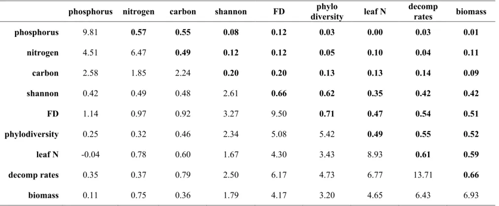
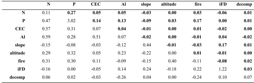
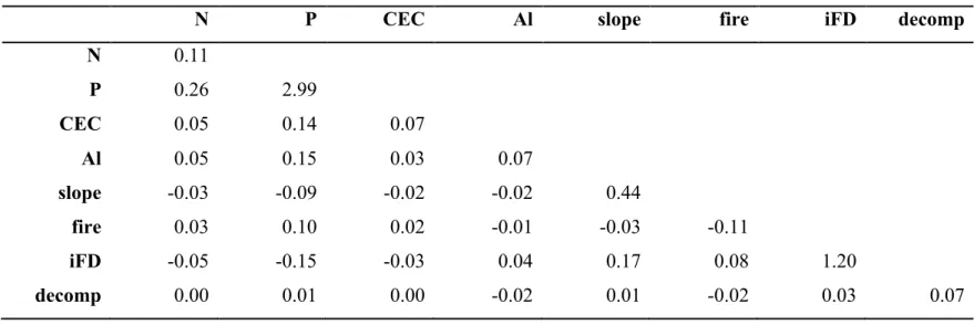
10SEM with MLE compares an observed covariance matrix with a model-implied one. The smaller 11
the differences between the two matrices, the better the model. When using MLE, data can be 12
provided as a correlation matrix (upper triangle in Table 1) with standard deviations (diagonal in 13
Table 1), as a covariance matrix (lower triangle in Table 1), or raw (a matrix with sample units in 14
rows and variables in columns). Even though covariances are used in the modelling, the raw data 15
must not deviate from the following assumptions: 16
Type 17
MLE requires normally distributed, and therefore continuous variables. Other types of data 18
common in ecology, like categorical and count data, can be estimated with alternative estimators, 19
especially from the weighted least squares family. Most introductory books give guidance when 20
Sample size 1
SEM needs large samples to provide accurate standard errors of parameter estimates. As a rule of 2
thumb for MLE, sample size should be > x20 the number of free parameters. A model with 15 3
parameters to be estimated ideally would have 300 cases. Bentler (1995) suggests that the 4
minimum sample size is x5 the number of free parameters (100 for a model with 20 free 5
parameters). For a small discussion on the implications of samples of different sizes on 6
parameter estimates, see Shipley (2000). In situations where it is not possible to collect a 7
sufficient amount of data for MLE, the researcher can resort to MLE coupled with bootstrapping 8
methods to generate unbiased standard errors of parameter estimates (Shipley 2000). 9
Collinearity 10
As usual, redundant variables are problematic and they should be eliminated or combined. The 11
same applies for variables with strong bivariate correlations. Scatterplots are useful for 12
identifying strong correlation. Multivariate collinearity is harder to spot. Kline (2010) suggests 13
building several multiple regression models, each with a different variable as the response and all 14
other variables as explanatory variables. A high coefficient of determination is an indication of 15
multicollinearity. Another way to detect multicollinearity in linear models is by using the 16
variance inflation factor (VIF; Fox & Monette 1992). VIF values greater than 10 suggest that 17
there is multicollinearity (Quinn & Keough 2002). Multicollinearity is dealt with very much the 18
same way as bivariate collinearity. One can either remove one of the variables that contribute to 19
the issue or combine related variables into a composite one. 20
Normality 21
density plots, and can be tested for with Kolmogorov-Smirnov test of goodness-of-fit or the 1
Shapiro-Wilk test (Legendre & Legendre 1998). Univariate normality does not guarantee 2
multivariate normality (Legendre & Legendre 1998). The generalised Shapiro-Wilk’s test 3
proposed by Villasenor Alva & Estrada (2009) can check for multivariate normality. 4
Highly skewed or kurtotic data can be transformed. See Zar (2009) for further 5
information. Alternatively, one can use robust maximum likelihood estimators (e.g., Satorra & 6
Bentler 1994), asymptotic distribution-free estimators, or bootstrapping. Shipley (2000) 7
discusses the issue of non-normality in biological datasets and provides guidance to alternative 8
estimation methods. 9
Outliers 10
Outliers can cause problems during parameter estimation. Identifying them and their cause is 11
often useful, therefore. Bivariate scatterplots, boxplots, and dotplots help find outliers. Another 12
method is calculation of z-scores (!!=!(!!−!!)/!), where ! is the raw score to be standardised,
13
! is the mean of the sample, and ! is the standard deviation of the sample) for each variable in 14
the set. In a normal distribution, 0.27% of the absolute standard scores are expected to have 15
values greater than 3.00. Deviations from this expected frequency (for instance, 1 when n = 370) 16
indicate the presence of possible outliers. MLE requires unstandardised data, so z-scores should 17
be used only to detect outliers. 18
Multivariate outliers are not necessarily outliers in the univariate frequency distributions. 19
When data are normally distributed in multivariate space, robust multivariate Mahalanobis 20
distances are expected to follow a !!"! distribution (Filzmoser et al. 2005). Data that fall outside 21
If outliers are present, one should carefully consider their source (sampling from a 1
different population, wrong data entry, etc) and then take action, such as data transformation, 2
outlier removal, or alternative estimators. 3
Covariance matrix 4
The covariance matrix used as input in SEM software must be positive-definite. If you are passed 5
a covariance matrix or are using one published in the literature, it is well worth checking this. 6
Some of the characteristics of positive-definite matrices are: 1) all covariances and correlations 7
are within bounds; 2) all eigenvalues (λn) are positive; and 3) the determinant of the matrix is 8
positive. These requirements are related to the iterative process during MLE, where the matrix is 9
inverted several times. 10
Please see the supplementary files for more information on how to detect and deal with 11
data related problems. Grace (2006) and Shipley (2000) further discuss the common issues posed 12
by biological data in the context of SEM. 13
Model estimation, fit, interpretation, and modification
14At this point, the model is specified and identified, there are sufficient data, and it meets the 15
assumptions of the estimator (here MLE). The next step is to pass to the estimation software the 16
covariance matrix and the proposed model structure. Although some software accept a 17
correlation matrix, the analysis of correlations requires constraints in the model and should be 18
Testing the measurement model using CFA 1
Instead of immediately estimating the full structural equation model (one-step method), it is best 2
to follow a multi-step approach. Multi-step approaches can help in finding sources of poor fit. 3
We present the two-step method proposed by Anderson & Gerbing (1988). The first step is 4
testing the measurement part of the structural equation model with a confirmatory factor analysis 5
(CFA) (e.g, Fig. 3). CFA is a type of SEM that focuses on the relationships between latent 6
variables and their indicators. In a CFA, all factors, that is are normally free to covary (e.g, two-7
headed arrows between latent variables in Fig. 3). The objective of this step is to find an 8
adequate measurement model before moving on to the structural model, so re-specification due 9
to poor fit is justified. A CFA indicates the need for model re-specification when indicators have 10
low standardised loadings, which may lead to poor fit with data. 11
One of the most important steps in parameter estimation is choosing adequate starting 12
values of free parameters. If the programme is given bad starting values, even the most robust 13
routines will fail to converge to an acceptable solution. Most software will automatically propose 14
adequate starting values. When this automation fails, it is up to the researcher to analyse each 15
causal relationship and to try to guess a plausible starting estimates. Kline (2010) gives 16
information on a way of manually guessing an adequate set of starting values. 17
From the starting parameter values, the estimator selects a set of close-by parameter 18
guesses, builds the expected covariance matrix, (!) and compares it to the observed covariance 19
matrix (!, Table 1). Programmes make this comparison by feeding both matrices to a fitting 20
function. For MLE, the fitting function is !!" =ln!−ln!+tr !!!! −!(!"+!"), where 21
!" is the number of observed exogenous variables and !" is the number of observed 22
endogenous variables. The closer S and ! are, the lower is the value of !
finds the set of estimates that gives the minimum value of !!", it stops and returns the 1
parameters. 2
The standard error of each parameter estimate is calculated using a Hessian matrix (a by- 3
product of the iterative fitting process). Standard errors provide access to the significance of each 4
estimate with simple t-tests. The value of fitting function !!" provides the MLχ!, which is a 5
measure of model fit with data. MLχ! =!×!!" where N is the number of observations in the 6
dataset. 7
When a model has adequate fit, the value of MLχ! has a P value greater than 0.05: the 8
observed and model-implied covariance matrices are not statistically different. The model in Fig. 9
3 had a non-significant MLχ! value (n = 210, MLχ! =22.98, != 0.52, and !! =24). 10
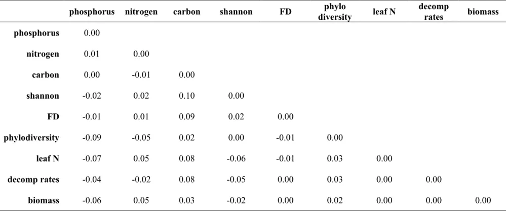
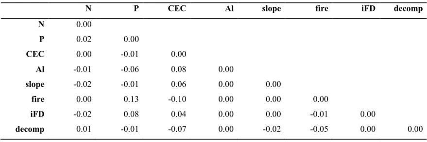
Before testing the structural part of the model, it is sensible to compare observed and 11
model implied bivariate correlations via the residual matrix (Table 2), obtained by subtracting 12
the observed correlation matrix (!) from the model implied one (!). Too large absolute 13
differences [Kline (2010) suggests a threshold of 0.10] indicate that the model does not properly 14
accommodate certain bivariate correlations, and can occur even when the MLχ! statistic suggests 15
good fit with data. In such cases, re-specification is warranted. 16
If the model does not have an acceptable fit, the researcher can consider alternative 17
models by freeing or setting some parameters. However, significant changes to the structure of 18
the model following poor fit should be reported in detail and supported by sound theory, as it is 19
easy to obtain good fit by adding or removing causal paths. 20
Following a satisfactory CFA, one should interpret the coefficients and assess latent 21
variable validity. Indicator loadings are interpreted as regression coefficients. For instance, in 22
an increase of 1 standard deviation in the latent construct will cause an expected 2.470 standard 1
deviation increase in the indicator. Unstandardised path coefficients may not be easily compared 2
due to differences in the scales of variables. Standardised effects, on the other hand, are more 3
easily compared since they are all in the same scale. Path coefficients can be either positive or 4
negative, indicating the nature of the relationships between two variables. Negative error 5
variances and disturbances are, however, an indication of Heywood cases, in which the software 6
converges to a solution without any apparent problems, but closer inspection reveals 7
interpretable results such as negative error variances. Possible causes of Heywood cases include 8
outliers, misspecification, nonidentification, poor starting values, and small sample size in 9
combination with too few indicators per latent variable (Kline 2010). 10
In the model in Fig. 3, only the covariance between soil fertility and community 11
functioning was not significantly different from zero (P < 0.05). Since we were interested only in 12
testing factor loadings before fitting the structural model, we left the non-significant parameter in 13
the model. If we were interested in this relationship, two routes are available: keeping the 14
parameter or removing it to try to improve model fit. However, non-significant parameters are 15
often best left, because even though they are not statistically different from zero, they contribute 16
to lower bivariate correlational residuals, rendering better fit with data (Kline 2010). 17
In the measurement model, in addition to the significance of each loading, one should 18
examine the reliability of the indicators: the amount of indicator variance explained by the latent 19
variable. For instance, the reliability of the variable phosphorus is given by one minus its 20
standardised error variance (1 – 0.375 = 0.625; Fig. 3). Thus, soil fertility accounts for 62.5% of 21
the variance of the manifest phosphorus. Reliability of an indicator is can also be calculated by 22
weigh up if the amount of variance explained is consistent with the theory driving the 1
specification. When reliability is low, one should reconsider one’s choice of latent or manifest 2
variables. See Grace (2006) and Grace et al. (2010) for more on reliability in ecological models. 3
Fitting the structural equation model 4
Following a satisfactory CFA, one proceeds to solving the structural equation model proposed. 5
The only difference between the CFA and the structural equation model is the relationships 6
between latent variables: the causal relations are used. Model fit and parameter estimates are 7
calculated and interpreted similarly. Any changes made to the measurement model resulting 8
from the CFA should be incorporated into the full structural equation model in the second step. 9
Since our CFA model was adequate, we did not make any changes to our measurement model. 10
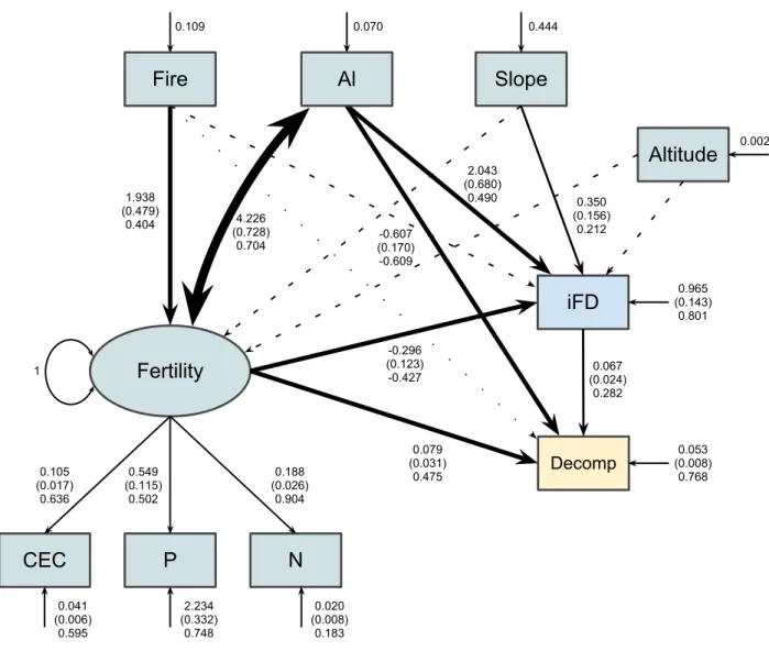
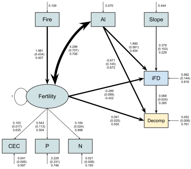
The structural equation model in Fig. 1 had good fit with data (!= 210, MLχ! =22.98, 11
! =0.52, and !" =24; Fig. 4). All parameters except the regression of soil fertility on
12
community functioning (!= −0.06, != 0.66; Fig. 4) were significant. Removing this 13
parameter from the model (i.e., setting its value to zero) only marginally increases the value of 14
the MLχ! statistic (n = 210, MLχ! = 23.17, ! =0.57, and !" =25). Thus, nested models,
15
which are models with the same set of variables but different causal configurations, can be 16
compared by subtracting the value of the MLχ! statistic of the more restrictive model from the 17
MLχ! of the less restrictive model, with significance assessed in χ!. In our case, the less 18
restrictive model is the one in Fig. 1, since the path between soil fertility and community 19
functioning is free (in the more restrictive model, the value of this parameter is fixed at zero). 20
The χ! difference in our case was χ! =23.17−22.98=0.19, for one degree of freedom
21
(!" = 25−24). The P value associated with this difference is 0.66. Thus, both models have
22
noteworthy differences between models. We retained the nonsignificant parameter since it makes 1
the model more consistent with previous knowledge, and possibly more generalisable to other 2
datasets. 3
Good fit is an indication that the model is capable of reproducing observed bivariate 4
relationships (Kline 2010), but does not necessarily indicate explanation of a large amount of the 5
variability of endogenous variables. For instance, the model in Fig. 4 explains only about 3% of 6
the variance of the latent variable biodiversity (!! = 1−0.966= !0.03; Fig. 4). The !! of an 7
endogenous variable is given by subtracting its standardised variance from 1. Such low explained 8
variance suggests that soil fertility alone is not a major cause of biodiversity. If we are interested 9
in explaining biodiversity, we should revisit the literature and include more predictors of 10
biodiversity. All other variables had a high amount of their variances explained by the model 11
(!! > 0.5).
12
The models in Fig. 3 and 5 are equivalent models. In the context of SEM, equivalent 13
models are models with the same set of variables but with different path directionality. The main 14
characteristic of equivalent models is that they produce the same value of fit statistics. For 15
instance, the difference between the models in Fig. 3 and 5 is the paths between latent variables. 16
The choice between mathematically equivalent models is, thus, based purely on theory and one 17
should thoroughly explain motives behind this decision. 18
Alternative measures of fit 19
The MLχ! statistic is a test of the exact-fit hypothesis between the observed and predicted 20
covariance matrices. Measures of approximate fit describe the degree of discrepancies between 21
model and data. The rationale for reporting approximate fit measures is that the power of the chi-22
between observed and predicted covariance matrices causing failure to fit statistics. Shipley 1
(2000) suggests that approximate fit measures are used after a model has failed exact-fit tests, to 2
show how close the rejected model is from a baseline model that fully reproduces observed data. 3
He adds that a major problem with these tests is the lack of evidence for the underlying 4
assumption that small specification problems translate into small deviations between data and 5
model-implied covariances. Also, there are no statistical tests to determine the cut-off values of 6
approximate fit measures. Researchers have to rely on the results of simulations as thresholds of 7
how “approximate” the model is from a correctly specified model. 8
Conclusion
9When used with the required caution, SEM yields a powerful set of tools that can be used to 10
generate models about the functioning of a system and, ultimately, reproduce, corroborate, and 11
fine-tune these frameworks to generalise our knowledge and increase our understanding of such 12
systems (Grace et al. 2010). 13
References
14Allen, B., Kon, M., & Bar-Yam, Y. (2009) A new phylogenetic diversity measure to generalizing 15
the Shannon index and its applications to phyllostomid bats. The American Naturalist, 16
174, 236-243. 17
Anderson, J. C. & Gerbing, D. W. (1988) Structural equation modeling in practice: A review and 18
recommended two-step approach. Psychological Bulletin, 103, 411-423. 19
Bentler, P. M. (1995). EQS structural equations program manual. Multivariate Software, 20
Boker, S. M., Neale, M. C., Maes, H. H., Wilde, M. J., Spiegel, M., Brick, T. R., Spies, J., 1
Estabrook, R., Kenny, S., Bates, T. C., Mehta, P., & Fox, J. (2011) OpenMx: An Open 2
Source Extended Structural Equation Modeling Framework. Psychometrika, 76, 306-317. 3
Carvalho, G. H., Batalha, M. A., & Petchey, O. L. (2011) stremo: Functions to help the process 4
of learning structural equation modelling. URL http://cran.r-5
project.org/web/packages/stremo/index.html [accessed on 12 April 2012] 6
Cianciaruso, M. V., Batalha, M. A., Gaston, K. J., & Petchey, O. L. (2009) Including 7
intraspecific variability in functional diversity. Ecology, 90, 81-89. 8
Filzmoser, P., Garrett, R. G., & Reimann, C. (2005) Multivariate outlier detection in exploration 9
geochemistry. Computers & Geosciences, 31, 579-587. 10
Fisher, R. A. (1925) Statistical Methods for Research Workers. Oliver and Boyd, Edinburgh. 11
Fox, J. & Monette, G. (1992) Generalized collinearity diagnostics. JASA, 87, 178-183. 12
Fox, J., Nie, Z., & Byrnes, J. (2012) sem: Structural Equation Models. URL http://cran.r-13
project.org/web/packages/sem/index.html [accessed on 12 April 2012] 14
Grace, J. & Pugesek, B. H. (1997) A structural equation model of plant species richness and its 15
application to a coastal wetland. The American Naturalist, 149, 436-460. 16
Grace, J. (2006) Structural Equation Modeling and Natural Systems. 1st edn. Cambridge 17
University Press, New York. 18
Grace, J., Anderson, T. M., Olff, H., & Scheiner, M. (2010) On the specification of structural 19
equation models for ecological systems. Ecological Monographs, 80, 67-87. 20
Jöreskog, K. G. (1970) A general method for analysis of covariance structures. Biometrika, 57, 21
239-251. 22