A new dataset for systematic assessments of climate change impacts as a function of global warming

(1)

GMDD

5, 3533–3572, 2012

A new dataset for systematic climate impact assessments

J. Heinke et al.

Title Page

Abstract Introduction

Conclusions References

Tables Figures

◭ ◮

Back Close

Full Screen / Esc

Printer-friendly Version

Interactive Discussion

Discussion

P

a

per

|

Dis

cussion

P

a

per

|

Discussion

P

a

per

|

Discussio

n

P

a

per

|

Geosci. Model Dev. Discuss., 5, 3533–3572, 2012 www.geosci-model-dev-discuss.net/5/3533/2012/ doi:10.5194/gmdd-5-3533-2012

Geoscientific Model Development Discussions

This discussion paper is/has been under review for the journal Geoscientific Model Development (GMD). Please refer to the corresponding final paper in GMD if available.

A new dataset for systematic

assessments of climate change impacts

as a function of global warming

J. Heinke1,2, S. Ostberg1, S. Schapho_ff1, K. Frieler1, C. M ¨uller1, D. Gerten1, M. Meinshausen1,3, and W. Lucht1,4

1

Potsdam Institute for Climate Impact Research, Telegraphenberg A62, 14473 Potsdam, Germany

2

International Livestock Research Institute, P.O. Box 30709, Nairobi, Kenya

3

School of Earth Sciences, McCoy Building, University of Melbourne, Victoria 3010, Australia

4

Department of Geography, Humboldt-Universit ¨at zu Berlin, Berlin, Germany

Received: 19 October 2012 – Accepted: 26 October 2012 – Published: 6 November 2012 Correspondence to: J. Heinke (jens.heinke@pik-potsdam.de)

(2)

GMDD

5, 3533–3572, 2012

J. Heinke et al.

Title Page

Tables Figures

◭ ◮

Back Close

Full Screen / Esc

Discussion

P

a

per

|

Dis

cussion

P

a

per

|

Discussion

P

a

per

|

Discussio

n

P

a

per

|

Abstract

In the ongoing political debate on climate change, global mean temperature change (∆Tglob) has become the yardstick by which mitigation costs, impacts from unavoided

climate change, and adaptation requirements are discussed. For a scientifically in-formed discourse along these lines systematic assessments of climate change impacts

5

as a function of∆Tglobare required. The current availability of climate change

scenar-ios constrains this type of assessment to a narrow range of temperature change and/or a reduced ensemble of climate models. Here, a newly composed dataset of climate change scenarios is presented that addresses the specific requirements for global as-sessments of climate change impacts as a function of ∆T_glob. A pattern-scaling

ap-10

proach is applied to extract generalized patterns of spatially explicit change in temper-ature, precipitation and cloudiness from 19 AOGCMs. The patterns are combined with scenarios of global mean temperature increase obtained from the reduced-complexity climate model MAGICC6 to create climate scenarios covering warming levels from 1.5 to 5 degrees above pre-industrial levels around the year 2100. The patterns are shown

15

to sufficiently maintain the original AOGCMs’ climate change properties, even though they, necessarily, utilize a simplified relationships between_∆Tgloband changes in local

climate properties. The dataset (made available online upon final publication of this pa-per) facilitates systematic analyses of climate change impacts as it covers a wider and finer-spaced range of climate change scenarios than the original AOGCM simulations.

20

1 Introduction

Impacts of anticipated future climate change on ecosystems and human societies are reason for major concern. Projections of such impacts are, however, characterised by uncertainties in greenhouse gas (GHG) emissions scenarios, their implementation in climate models (involvinginter aliastructural uncertainties of climate models) and their

25

(3)

GMDD

5, 3533–3572, 2012

J. Heinke et al.

Title Page

Tables Figures

◭ ◮

Back Close

Full Screen / Esc

Discussion

P

a

per

|

Dis

cussion

P

a

per

|

Discussion

P

a

per

|

Discussio

n

P

a

per

|

the Intergovernmental Panel on Climate Change’s Working Group II report (Parry et al., 2007), assessments commonly lack systematic quantification of impacts as a function of global warming, as only a small and often opportunistic selection of available climate change scenarios is employed. This hampers direct comparisons between studies (e.g. M ¨uller et al., 2011) and also our understanding of how impacts and their likelihood

5

change over time or as a function of global mean temperature (Tglob). The magnitude

of impacts to be expected given specific degrees of T_glob rise has gained increasing attention in recent years due to the United Nations Framework Convention on Climate Change’s stipulation to prevent “dangerous climate change” and the ensuing discus-sion on whether this would be met by a 2 degree mitigation target (rather than, e.g.

10

a 1.5 or 3 degree target). Besides requiring an understanding of how impacts individ-ually and collectively accumulate with increasingTglob, an understanding of the

conse-quences of missing a given target is important for this discussion (e.g. Mann, 2009). Compilations of individual impact studies have helped to illustrate the underlying “rea-sons for concern” (Smith et al., 2009) but do not provide the consistent quantitative

15

information needed.

In view of the importance of mitigation targets for the debate on climate change mit-igation and the substantial investments required to meet them, the number of studies that scrutinise systematically and consistently the worldwide impacts to be expected as a function of_∆Tglob, let alone their uncertainties, is surprisingly small. Examples for

20

global assessments of impacts ordered along ∆Tglob and derived with single impact

modelling frameworks are those by Arnell et al. (2011); Gosling et al. (2010), and Mur-ray et al. (2012) for freshwater availability, and those by Gerber et al. (2004); Scholze et al. (2006); Sitch et al. (2008), and Heyder et al. (2011) for ecosystems and the carbon cycle. Other assessments have focused on diverse impacts given a ∆Tglob of

25

4 degrees (see New et al., 2011).

While much of the uncertainty inTglobis attributable to the fact that the exact

(4)

GMDD

5, 3533–3572, 2012

J. Heinke et al.

Title Page

Tables Figures

◭ ◮

Back Close

Full Screen / Esc

Discussion

P

a

per

|

Dis

cussion

P

a

per

|

Discussion

P

a

per

|

Discussio

n

P

a

per

|

Circulation Models (AOGCMs) additionally contributes to uncertainty in regional tem-perature and precipitation changes associated with a given∆Tglob (Hawkins and

Sut-ton, 2011). Most of above-mentioned studies could account only partly for the latter, as they either relied on a small selection of AOGCMs or grouped larger ensembles ac-cording to the∆Tglobreached by the individual AOGCMs by the end of their simulation

5

period (e.g. Scholze et al., 2006). More rigorous assessments of impacts as a function of global warming are generally limited by the availability of AOGCM simulations in the CMIP3 archive. The range of warming levels covered by the different AOGCMs differs widely and the increase inTglobover the twenty-first for the highest emission scenario

A2 is only 3.4 in the multi-model mean (Meehl et al., 2007).

10

Overall, systematic assessments of climate change impacts as a function of global warming require that a large∆Tglobrange be covered (from, e.g. 1.5 to 5 degrees), and

that the respective ∆Tglob levels are reached at around the same time. Furthermore,

for every _∆Tglob level information on local changes in key climate variables (such as

temperature, precipitation, radiation or cloudiness) should consider an AOGCM

multi-15

model ensemble as large as possible, in order to account for the substantial climate model-structural uncertainty. Such consistent information is not directly available in the existing CMIP3 and CMIP5 climate databases – it requires fusion of comprehen-sive datasets on climate change patterns from different AOGCMs with different∆Tglob

trajectories (and underlying emissions trajectories), information on observed climate

20

(without AOGCM biases), and reduced-complexity models able to overcome the high computation requirements of AOGCMs.

To address some of these features, a number of studies (e.g. Gosling et al., 2010; Murray et al., 2012) have used emulated rather than original AOGCM output, calculated with the so-called “pattern-scaling” technique (Mitchell, 2003) that makes use of the

25

correlation between local long-term mean changes of climate variables and _∆Tglob.

Scaling coefficients were found to differ spatially and seasonally, but particularly for temperature they are nearly independent of the GHG emission scenarios considered and sufficiently accurate over a wide range of ∆Tglob (Solomon et al., 2009; Mitchell,

(5)

GMDD

5, 3533–3572, 2012

J. Heinke et al.

Title Page

Tables Figures

◭ ◮

Back Close

Full Screen / Esc

Discussion

P

a

per

|

Dis

cussion

P

a

per

|

Discussion

P

a

per

|

Discussio

n

P

a

per

|

2003; Huntingford and Cox, 2000). Hence, pattern-scaling is an efficient method to generate climate scenarios for systematic analyses of climate impacts as a function of

∆Tglob.

Using a comprehensive pattern-scaling approach covering monthly mean surface temperature, cloudiness and precipitation, we here present a newly collated global

5

dataset of climate change scenarios that overcomes most of the above problems and is suited for systematic, macro-scale impact assessments with empirical or process-based impact models. It is process-based on GCM-specific scaling patterns that are combined with time series of∆Tglobas generated by a reduced-complexity climate model,

MAG-ICC6 (Meinshausen et al., 2011a). The emissions scenarios are designed such that

10

each of eight_∆Tglob levels (1.5 to 5 degrees above pre-industrial levels in 0.5 degree

steps) is reached by 2100. Monthly climate anomaly patterns are derived for each of 19 AOGCMs available from the World Climate Research Programme’s (WCRP’s) Cou-pled Model Intercomparison Project phase 3 (CMIP3) multi-model dataset. Scaling the derived generic change patterns per degree of global mean warming with the∆Tglob

tra-15

jectories generates transient time series of climate anomalies up to 2100. This dataset enables consistent analyses of impacts as a function of_∆Tglob at the end of the

cen-tury, and improved comparability of climate patterns and resulting impacts for given Tgloblevels.

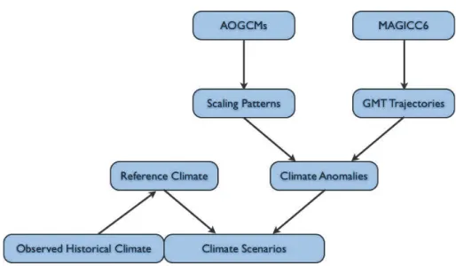
2 Methods

20

Figure 1 sketches the steps of data processing and combination involved in the creation of the climate scenarios, as described in detail in the following sections. Section 2.1 describes the extraction of scaling patterns – i.e. the spatial fields of local (monthly) climate change per one degree of∆Tglob– from AOGCM simulations. Section 2.2

cov-ers the generation ofTglobtrajectories by the MAGICC6 model, and their combination

25

(6)

GMDD

5, 3533–3572, 2012

J. Heinke et al.

Title Page

Tables Figures

◭ ◮

Back Close

Full Screen / Esc

Discussion

P

a

per

|

Dis

cussion

P

a

per

|

Discussion

P

a

per

|

Discussio

n

P

a

per

|

local anomalies with data on observed variability and climatological means to generate climate scenarios harmonised with historical observations, covering the entire global land area.

2.1 Derivation of scaling patterns from AOGCM simulations

The basic relationship of the pattern-scaling approach used here, building on previous

5

methods by, e.g. Huntingford and Cox (2000), is given in Eq. (1):

∆V(x,m,y)= ∆Tglob(y)·V

∗

(x,m) (1)

where∆V(x,m,y) denotes the anomaly, i.e. the change in the long-term mean of vari-ableV (e.g. air temperature) for locationx and month m in yeary.∆Tglob(y) denotes

10

the change in global mean temperature in yeary relative to preindustrial conditions; and V∗

(x,m) is the scaling coe_fficient, i.e. the change in V per degree of ∆Tglob for

each location and month but independent of time (y). In other words, a linear relation-ship between local mean changes of climate variables and changes in global mean temperature is assumed. The entirety of all scaling coefficientsV∗

(x,m) for a particular

15

variable and AOGCM is referred to asscaling pattern.

The estimation of V∗(x,m) is based on the assumption that deviations from the pre-industrial mean ∆V(x,m,y) are composed of the change in the long-term mean ∆V(x,m,y) and natural interannual variabilitye(x,m,y) around it. In combination with Eq. (1) this yields a simple linear regression model that forms the basis for estimating

20

scaling coe_fficients from AOGCM simulations:

∆V(x,m,y)=V∗

(x,m)·∆T_glob(y)+e(x,m,y) (2)

For the estimation ofV∗

(x,m) from AOGCM simulations the monthly data were lin-early interpolated from their original spatial resolution to the target resolution used here,

25

(7)

GMDD

5, 3533–3572, 2012

J. Heinke et al.

Title Page

Tables Figures

◭ ◮

Back Close

Full Screen / Esc

Discussion

P

a

per

|

Dis

cussion

P

a

per

|

Discussion

P

a

per

|

Discussio

n

P

a

per

|

relative to the long-term climatological means of the pre-industrial control run (without any anthropogenic forcing) available for all AOGCMs for between 100 and 990 simula-tion years.∆Tglob(y) are estimated as the annual area-weighted global average

(includ-ing oceans) of∆T(x,m,y). As the extraction of patterns ofV∗

(x,m) is based on linear regression, the residual errorse(x,m,y) are in fact a mixture of interannual variability

5

and the imperfection of the regression model. The quality of the fit obtained can thus be evaluated by comparison of residual errors and respective interannual variability estimated from the control simulation (see Sect. 3.2).

We applied the above methodology to monthly mean near-surface air temperature, cloudiness and precipitation. Additionally, we studied logarithmic precipitation to

re-10

flect an alternate assumption of exponential rather than linear precipitation change. In the logarithmic precipitation regression model, exclusion of dry months alters the esti-mated trend of precipitation amounts under climate change. This problem is not purely of numerical nature but highlights that the change in frequency of rain months and the change in the rainfall amounts for rain months represent qualitatively different

infor-15

mation that should be addressed separately. Hence, we removed dry months (<1 mm per month) from the linear fit (Eq. 2) of both precipitation and logarithmic precipitation so that both regression models capture the change in rainfall amounts for rain months only.

Building on the basic principle of the pattern-scaling approach, the change in

fre-20

quency of rain months (p) was considered separately by applying a logistic regression model, in which probabilities are logit-transformed and related to a linear predictor term, which gives a generalised linear regression model:

logit (p(x,m,y))=ln

_p₍_x_,_m_,_y₎

1−p(x,m,y)

=β0(x,m)+β

∗

(x,m)·_∆T_glob(y) (3)

25

whereβ₀(x,m) andβ∗

(8)

GMDD

5, 3533–3572, 2012

J. Heinke et al.

Title Page

Tables Figures

◭ ◮

Back Close

Full Screen / Esc

Discussion

P

a

per

|

Dis

cussion

P

a

per

|

Discussion

P

a

per

|

Discussio

n

P

a

per

|

month occurrence we used the glm() function (Generalized Linear Model) from the core package “stats” of the statistical software R (R Development Core Team, 2011).

2.2 Construction of climate scenarios from derived patterns

2.2.1 Construction of scenarios of global mean temperature increase

The derived scaling patterns V∗(x,m) for the different climate variables are the basis

5

for constructing time series of local anomalies of climate variables consistent with pre-scribedTglobtrajectories. We ran the MAGICC6 model to obtain physically and

system-ically plausible∆Tglob trajectories and corresponding trajectories of atmospheric CO2

concentration ([CO2]) (required for some impact models). MAGICC6 is a highly efficient

reduced-complexity carbon cycle climate model (Meinshausen et al., 2011a) that has

10

been shown to closely emulate mean results of complex AOGCMs from the CMIP3 data base (Meinshausen et al., 2011b). Here, MAGICC6 was used to calculate∆Tglob and

[CO₂] for a large number of artificial emissions pathways constructed as described by (Meinshausen et al., 2009). For that purpose MAGICC’s carbon cycle parameters were adjusted to reproduce the Bern carbon cycle model and the climate model parameters

15

were chosen to reproduce the median responses of the CMIP3 AOGCM ensemble. Climate sensitivity, for example, was set to 3.0 K.

From the generated large ensemble of pathways we selected those pairs of ∆Tglob

and [CO₂] trajectories where ∆T_globpathways reached 1.5, 2.0, 2.5, 3.0, 3.5, 4.0, 4.5, and 5.0 degrees above pre-industrial level in the period 2086–2115 (see Fig. 2). The

20

definition of the temperature target for a period rather than for a single year (e.g. 2100) was chosen because the analysis of time periods is common practice in impact assess-ments to avoid spurious e_ffects from inter-annual variability. 30 yr is a typical length used in impact studies in hydrology, agriculture, and ecosystems, for which our new data set is designed.

25

An outstanding feature in Fig. 2 that illustrates the above-mentioned physical and systemic plausibility is the initially stronger increase in Tglob in the lower than in the

(9)

GMDD

5, 3533–3572, 2012

J. Heinke et al.

Title Page

Tables Figures

◭ ◮

Back Close

Full Screen / Esc

Discussion

P

a

per

|

Dis

cussion

P

a

per

|

Discussion

P

a

per

|

Discussio

n

P

a

per

|

high temperature scenarios. Stronger mitigation scenarios tend to show a much faster decrease in aerosol emissions than in CO2 emissions as a rapid decrease of CO2

emissions is accompanied by a switch to “cleaner” sources of energy. This correlation between CO₂ and aerosol emissions results from our use of the Equal Quantile Walk method (Meinshausen et al., 2006) to create the different emission profiles that led

5

to the various warming levels. The drop in aerosol emissions in combination with the much shorter residence time of aerosols in the atmosphere results in a rapid reduction of the aerosol cooling effect (see Ramanathan and Feng, 2008). As a consequence, the committed warming from current [CO2] can unfold before a further reduction of CO2

emissions eventually results in an overall decrease in radiative forcing and temperature.

10

Conversely, the CO₂ emissions in the high temperature scenarios are accompanied by high aerosol emissions that maintain the cooling effect. Besides the possibility to produceTglob scenarios together with consistent [CO2] trajectories, the consideration

of such e_ffects is the major advantage of applying MAGICC6 in this study.

2.2.2 Construction of local time series of climate anomalies

15

Local time series of climate anomalies for the four climate variables were obtained by multiplying the scaling coefficients V∗

(x,m) and the yearly ∆T_glob values for each scenario (Eq. 1). Because the time series of anomalies obtained are harmonised with climate observations in the next step (see Sect. 2.3), it is necessary to account for the climate change signal already present in these observations. Anomalies are therefore

20

calculated relative to the last year of observations, 2009. This is achieved by subtract-ing theTglobincrease above pre-industrial level for the year 2009 (∼0.9 K) from theTglob

trajectories of the MAGICC6 scenarios before multiplying them with the anomaly pat-terns. In all cases anomalies were only calculated if the significance level of the slope of the regression model is>0.9; otherwise they were set to zero.

25

(10)

GMDD

5, 3533–3572, 2012

J. Heinke et al.

Title Page

Tables Figures

◭ ◮

Back Close

Full Screen / Esc

Discussion

P

a

per

|

Dis

cussion

P

a

per

|

Discussion

P

a

per

|

Discussio

n

P

a

per

|

these variables. For cloudiness this problem is less critical as it is not used directly in impact models but serves, among other parameters, as a proxy for atmospheric trans-missivity and etrans-missivity in the estimation of radiation budgets. We therefore consider a simple capping of anomalies to prevent the exceedance of upper and lower limit a sufficiently accurate solution. In contrast to cloudiness precipitation is an essential

5

variable and calculation of anomalies that would result in physically implausible nega-tive precipitation rates should be avoided from the beginning. Anomalies for decreasing precipitation are therefore estimated from the regression models for logarithmic precip-itation, which is equivalent to the assumption of exponential precipitation decrease. As there is no indication that precipitation would increase exponentially withTglob,

pre-10

cipitation increases are estimated from the linear regression models for untransformed precipitation. For small change rates, the linear and the exponential approach yield very similar anomalies while for large change rates the linear approach avoids unrealistically augmented increases and the exponential approach avoids negative precipitation rates (see also Watterson, 2008). For estimating rain month frequency anomalies, changes

15

in the linear predictor term of Eq. (3), i.e. anomalies of logit probabilities, were calcu-lated. These obtained anomalies can be used without restrictions, as the range of logit probabilities is unconstrained. For the transformation into actual frequency anomalies see Sect. 2.3.4.

2.3 Creation of climate scenarios from observed climate and derived climate

20

anomalies

To facilitate transient impact model runs, the anomaly time series – i.e. the combination of smoothTglobtrajectories and anomaly pattern regression models – need to be

com-bined with an observed mean climatology and information on interannual variability. Here, observations of temperature and cloudiness over land were taken from the CRU

25

TS3.1 global climate data set (Mitchell and Jones, 2005). Observations of monthly pre-cipitation over land were taken from the GPCC data set version 5 (Rudolf et al., 2010). Because GPCC and CRU datasets have a slightly di_fferent land mask, GPCC data

(11)

GMDD

5, 3533–3572, 2012

J. Heinke et al.

Title Page

Tables Figures

◭ ◮

Back Close

Full Screen / Esc

Discussion

P

a

per

|

Dis

cussion

P

a

per

|

Discussion

P

a

per

|

Discussio

n

P

a

per

|

were adjusted to the CRU land mask (67 420 grid cells) by filling up missing cells by interpolation. For this, the five neighbouring cells with the highest weight – calculated from distance and angular separation (New et al., 2000) – within a 450 km radius were used. If <5 values were available, the interpolation was performed on this reduced data basis; if<2, the precipitation from the CRU TS3.1 data set was used. Grid cells

5

only present in the GPCC land mask but not in the CRU land mask were excluded. Altogether, 767 grid cells were introduced by interpolation, 298 grid cells were directly taken from CRU TS3.1, and 1013 grid cells were omitted from the GPCC dataset.

A 106-yr time series covering the scenario period (2010–2115) was composed as a random sequence of years from historical observations of the period 1961–2009. To

10

preserve intraannual autocorrelation, spatial coherence, and correlation among climate variables, all months and grid cells for all climate variables were taken from the same year. Prior to resampling, the trend in temperature was removed in a way that the de-trended time series of temperature are representative for the climatologic mean of year 2009 obtained from the trend analysis. In the process of data preparation, observations

15

of precipitation and cloudiness were found to exhibit strong interannual/interdecadal variability, which negatively a_ffects the robustness of estimated trends. In order to avoid spurious effects from removing these trends, the original data were used directly for generating the reference time series for cloudiness and precipitation. The time series of resampled observations obtained are assumed to represent variability and

climatol-20

ogy for the reference year 2009, to be consistent with the reference year for the derived anomalies. In the following this dataset is referred to as “reference time series”. This consistency between the constructed reference time series, the derived anomaly pat-terns, and observations allows for harmonisation of historic observations with future climate projections and thus for transient impact model runs.

25

(12)

GMDD

5, 3533–3572, 2012

J. Heinke et al.

Title Page

Tables Figures

◭ ◮

Back Close

Full Screen / Esc

Discussion

P

a

per

|

Dis

cussion

P

a

per

|

Discussion

P

a

per

|

Discussio

n

P

a

per

|

absolute signal is progressively altered with the relative approach. This alteration is an expression of the adjustment of the absolute anomaly derived from a biased base level in the AOGCM to the observed level, which is the actual motivation for using the relative approach. The relevance of this adjustment is particularly apparent where decreases from overestimated levels in the AOGCM are applied to lower observed levels.

How-5

ever, for the reverse case – increases from underestimated levels – this approach is less favourable as it may lead to an unrealistic augmentation of the absolute anomaly. Building on previous work by F ¨ussel (2003), the methodology applied here aims at bal-ancing the artificial alteration of the original signal and the necessary adjustment due to AOGCM biases (see also Gerten et al., 2011, where a similar approach was used).

10

2.3.1 Temperature

Temperature anomalies are commonly treated as absolute changes, thus they are sim-ply added to the reference time series:

Tscen=Tref+Tanom (4)

15

whereTscen,Tref, andTanom are the temperature time series of the scenario, the

refer-ence time series, and the anomalies, respectively. As temperature biases in AOGCMs are very small compared to absolute temperature levels, the application as relative anomalies would yield very similar results.

2.3.2 Cloudiness

20

For cloudiness, anomalies were applied as relative changes. Due to the problem of augmentation of anomalies when applied as relative change to higher observed lev-els, there is a risk of exceeding the upper 100 % limit in these cases. Increases in cloudiness are therefore applied as relative decreases of cloudlessness, i.e. 100 % – cloudiness:

25

(13)

GMDD

5, 3533–3572, 2012

J. Heinke et al.

Title Page

Tables Figures

◭ ◮

Back Close

Full Screen / Esc

Discussion

P

a

per

|

Dis

cussion

P

a

per

|

Discussion

P

a

per

|

Discussio

n

P

a

per

|

Cldscen=    

  

Cldref·

Cld_base+Cld_anom

Cld_base for Cldanom<0

100−(100−Cldref)· 100−

Cld_base+Cld_anom

100−Cld_base for Cldanom>0

(5)

with Cldscen, Cldref, and Cldanomdenoting the cloudiness time series of the scenario, the

reference time series, and the anomalies, respectively. As the absolute anomalies are relative to the base year 2009, Cldbase represents the AOGCM’s climatological mean

5

for the year 2009. The estimation of Cldbase is based on the climatological mean of

the control run to which the cloudiness anomaly for a 0.9 K warming is added (see Sect. 2.2.2).

2.3.3 Precipitation

Precipitation is the most problematic variable for applying anomalies because of its

10

relevance as key variable in impact assessments and the partially very large biases in simulated present-day precipitation. In cases where simulated precipitation in the control run is very low, small absolute increases are very large if expressed as rel-ative changes. If these are used to scale significantly higher observed precipitation rates, the applied absolute anomalies become unrealistically large. Other studies have

15

therefore proposed to use absolute changes or limit the relative changes in such cases (Carter et al., 1994; Hulme et al., 1995). Since the problem primarily arises from the underestimation of present precipitation rates by AOGCMs, a seamless transition from a relative towards an absolute interpretation of anomalies depending on the degree of underestimation is used here:

20

Pscen=Pref·



1+

Panom

Pref

!

Pref

Pbase

!λ

(14)

GMDD

5, 3533–3572, 2012

J. Heinke et al.

Title Page

Tables Figures

◭ ◮

Back Close

Full Screen / Esc

Discussion

P

a

per

|

Dis

cussion

P

a

per

|

Discussion

P

a

per

|

Discussio

n

P

a

per

|

with

λ=

 

 r

P_base

P_ref forPbase< Pref

1 forPbase≥Pref

(7)

with Pscen, Pref, and Panom denoting the precipitation time series of the scenario, the

reference time series, and the anomalies, respectively; andPrefandPbasedenoting the

5

climatological mean of the reference time series and the year 2009 in the AOGCM, re-spectively. Estimation ofP_base is analogous to estimation of Cld_base(see Sect. 2.3.2). The exponent λ determines the degree to which an anomaly is applied as absolute or relative change. If λ=1, Eq. (6) is equivalent to the relative interpretation of pre-cipitation anomalies. If present prepre-cipitation is underestimated by the AOGCM, lower

10

values ofλ apply to diminish the applied relative anomaly. If λapproaches zero, the factor applied to the values of the reference time series results in a shift of its mean equal to the absolute anomalyPanom. Note that the form of Eq. (6) implies that changes

in mean precipitation are always accompanied by changes in standard deviation, i.e. interannual variability.

15

2.3.4 Rain month frequency

Based on the logistic regression model estimated from the AOGCM simulations, the probability of rain month occurrence was estimated for each month of the scaled sce-nario time series as follows:

pscen(y)=

ez

1+ez with z=logit (pref)+β

∗

·∆T_glob(y) (8)

20

wherepscen(y) is the probability of yeary in the scenario to be a rain month andpref

the probability of rain month occurrence in the reference time series – i.e. the fraction of rain months in that series. In cases whereprefis either 0 or 1, logit (pref) cannot be

(15)

GMDD

5, 3533–3572, 2012

J. Heinke et al.

Title Page

Tables Figures

◭ ◮

Back Close

Full Screen / Esc

Discussion

P

a

per

|

Dis

cussion

P

a

per

|

Discussion

P

a

per

|

Discussio

n

P

a

per

|

calculated and was set to a value of−7 and 7, respectively. This is equivalent to values

forpref of about 1/1100 and 1−1/1100, respectively. The termβ

∗

·_∆T_glob(y) denotes

the anomaly of the logit rain month probability estimated from the logistic regression model andTglob anomalies (see Sect. 2.2.2). Because the intercept and the slope of

the logistic regression model are both estimated by fitting the model to the scenario

5

data, extreme values are sometimes obtained forβ∗

where rain month probability is 0 or 1 and some singular dry or rain months occur towards the higher end of the tem-perature range. When used with the estimated interceptβ0, these slopes correspond

to very small changes in rain month probability but produce unrealistically augmented probability changes when applied topref in Eq. (8). In order to avoid this effect, only

10

slopes with a corresponding estimate for the intercept between−7 and 7 were applied;

otherwise no change was applied. This rule applied to about 5.5 % of all significant estimates forβ∗

.

The application of pscen to the reference time series entails the removal of excess

and the introduction of additional rain months by means of a stochastic process. For

15

this procedure a random sequence w(y) of uniformly distributed numbers between 0 and 1 is generated, which serves as a decision criterion on whether a rain month is introduced or removed in yeary. Ifpscen(y) is smaller thanprefa rain month is removed

if

w(y)≥pscen(y)

pref

(9)

20

Conversely, ifpscen(y) is larger thanpref, a rain month is introduced if

1−w(y)≥1−pscen(y)

1−p_ref (10)

The precipitation event to be introduced is randomly chosen from the precipitation

25

(16)

GMDD

5, 3533–3572, 2012

J. Heinke et al.

Title Page

Tables Figures

◭ ◮

Back Close

Full Screen / Esc

Discussion

P

a

per

|

Dis

cussion

P

a

per

|

Discussion

P

a

per

|

Discussio

n

P

a

per

|

series has no rain month at all, a synthetic rainfall distribution is generated by interpo-lation from up to five neighbour cells with at least one precipitation event in their distri-bution. The selection criterion for these cells was taken to be the highest interpolation weight from all cells within a radius of 450 km. Interpolation weights were calculated as in New et al. (2000) with account for distance and angular separation.

5

In order to preserve the spatial and temporal coherence of the precipitation field, the same random number sequence w(y) was used for all grid cells and months of the year. The rationale behind this procedure is that for neighbouring cells with similar pscen(y) and pref, rain months get removed or inserted in the same year. In order to

avoid an overlap with the removal of rain months, however, the reflected sequence 1−

10

w(y) was used as decision criterion for the introduction of rain months. The procedure was applied prior to the scaling of precipitation amounts described in the preceding sections. Average reference precipitation was calculated for the modified reference time series.

2.3.5 Wet-day frequency

15

An additional information required by many impact models is the number of wet days per month. Due to the sparse availability of daily rainfall data from AOGCMs and strong biases in frequency distribution of rainfall intensities in many AOGCMs, this information is hard to extract from these models. The number of wet days per month is therefore estimated based on New et al. (2000) using the relationship between monthly

precipi-20

tation sum and number of wet days:

WD=WDobs

P

Pobs

!γ

(11)

whereP and WD represent the precipitation sum and the estimated number of wet days of a month and grid cell, respectively. The exponentγ is assumed to be 0.45,

25

which was found by New et al. (2000) to yield best results. The values WD_obs andPobs

(17)

GMDD

5, 3533–3572, 2012

J. Heinke et al.

Title Page

Tables Figures

◭ ◮

Back Close

Full Screen / Esc

Discussion

P

a

per

|

Dis

cussion

P

a

per

|

Discussion

P

a

per

|

Discussio

n

P

a

per

|

represent the observed 1961–1990 mean monthly wet day frequency and precipitation sum, respectively. The former was derived from CRU TS3.1 (Mitchell and Jones, 2005) and the latter from GPCC version 5 (Rudolf et al., 2010). The means were calculated over the entire 30-yr period, including totally dry months. Because the data sets for wet days and precipitation are based on di_fferent station networks they are not fully

5

consistent, i.e. there are cases where rain months have zero wet days (and vice versa). The absolute minimum for WDobs is the fraction of rain months in the 30-yr period,

which means that at least one wet day has to exist for each rain month. If the estimate of WDobs is smaller than that, it was set to that minimum. This estimation procedure

delivers conservative estimates of wet day frequency for the scenario period since the

10

relationship between wet day frequency and monthly precipitation sum is assumed to be constant over time.

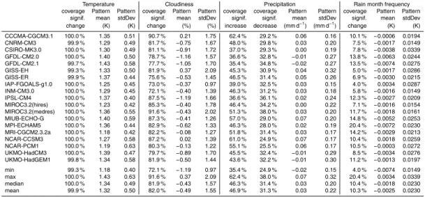
3 Results and discussion

3.1 Properties of scaling patterns extracted from AOGCM simulations

The scaling patterns extracted from AOGCM simulations are the core component of the

15

scenario-building described in this paper. They provide information on spatial and tem-poral heterogeneity of climate change signals for primary climate variables as projected by different AOGCMs. In this section, an overview is given of the spatial coverage of fits that are significant and of basic properties of the derived patterns (mean and standard deviation). The focus is primarily on a comparison of the different climate variables with

20

some indication of the inter-model spread. A comprehensive overview with values for individual AOGCMs is presented in Table 1.

An apparent difference between the climate variables is the spatial and temporal coverage of significant slope parameters of the regression models obtained from the AOGCM simulation. As described in Sect. 2.2.2, only slope estimates with a statistical

25

(18)

GMDD

5, 3533–3572, 2012

J. Heinke et al.

Title Page

Tables Figures

◭ ◮

Back Close

Full Screen / Esc

Discussion

P

a

per

|

Dis

cussion

P

a

per

|

Discussion

P

a

per

|

Discussio

n

P

a

per

|

representative for a specific area (size of grid cell) and a specific time period of the year (length of month). In order to assess the spatial and temporal coverage of significant slope estimates, the product of area and duration for each significant slope is calculated and summed up. The sum is related to the product of total land area and length of the year to arrive at a percentage of spatial and temporal coverage.

5

Averaged over all AOGCMs, spatial and temporal coverage of significant slopes is 99.9 %, 82.0 %, and 78.2 % for temperature, cloudiness and precipitation, respectively (value for precipitation composed of 46.9 % significant increases in the linear case and 31.3 % significant decreases in the logarithmic case; Table 1). The average coverage of significant slopes for the logistic regression models for rain month probability is 10.9 %

10

and 10.3 % if regression models with extreme intercepts are excluded (see Sect. 2.3.4). Although there is considerable variation in spatial coverage of significant fits among individual AOGCMs (see Table 1) the relative magnitude of coverage for the different variables is consistent over all models. Near full coverage is found for temperature, followed by moderate to high coverage for cloudiness and precipitation (including both

15

increases and decreases). Coverage of significant precipitation increases is in all cases higher than for decreases although values are similar in some cases. In all cases, coverage of significant changes of rain month frequency is smallest.

Although the coverage of significant changes for cloudiness, precipitation, and rain month frequency is significantly lower than for temperature, this must not be interpreted

20

as an indication of limited applicability of the pattern-scaling approach for these vari-ables. A major difference between temperature and the other variables is that for the former only positive trends occur while the other variables display a mixture of positive and negative trends (see Figs. 3–6). This implies the existence of transition zones be-tween areas with positive and negative trends in the monthly fields where trends are de

25

facto zero and therefore no significant slopes can be found. In addition, cloudiness and precipitation both exhibit strong interannual variability that tends to mask weak trends that primarily occur around such transition zones. Similarly, the estimation of parame-ters of the logistic regression model for change of rain month frequency is hampered

(19)

GMDD

5, 3533–3572, 2012

J. Heinke et al.

Title Page

Tables Figures

◭ ◮

Back Close

Full Screen / Esc

Discussion

P

a

per

|

Dis

cussion

P

a

per

|

Discussion

P

a

per

|

Discussio

n

P

a

per

|

by the stochastic nature of this variable. Moreover, vast areas with a rain month fre-quency of 100 % (e.g. in the high latitudes and the wet tropics) remain una_ffected by the occurrence of dry months under climate change (Fig. 6).

For each derived anomaly pattern two statistics – mean and standard deviation –are calculated in order to characterise the patterns. We took into account the spatial and

5

temporal coverage of the individual slopes – i.e. by weighting them with the respective cell area and length of month. Because the aim is to illustrate the properties of the entire pattern as it is applied, grid cells and months without a significant slope are included as zero values.

Averaged over all AOGCMs the mean anomaly of temperature increase over land is

10

estimated to be 1.32 K per 1 K increase ofTglob(from 14.0

◦

C in the reference time se-ries). BecauseTglobanomalies and local temperature anomalies used in the regression

are estimated from the same data the value demonstrates that the land surface heats up much more than the whole of the global surface. This phenomenon is well known and is caused by the higher heat storage capacity of the oceans, which cause them to

15

heat up less (Lambert and Chiang, 2007). Although temperature trends are found to be always positive over land (Fig. 3) there is considerable heterogeneity in the degree of warming in different regions and times of the year. This heterogeneity is captured by the pattern’s standard deviation, which on average over all AOGCMs is 0.5 K. The mean and standard deviation for individual models are in the range of 1.18–1.43 and

20

0.40–0.63, respectively (Table 1).

The prevalence of a clear mean signal in the pattern is unique to temperature among the variables considered here. For cloudiness the average pattern mean is−0.49 % –

less than 1 % of the mean cloudiness over land in the reference time series (55.3 %). The relatively small mean change is contrasted by a higher standard deviation of

25

(20)

GMDD

5, 3533–3572, 2012

J. Heinke et al.

Title Page

Tables Figures

◭ ◮

Back Close

Full Screen / Esc

Discussion

P

a

per

|

Dis

cussion

P

a

per

|

Discussion

P

a

per

|

Discussio

n

P

a

per

|

For the calculation of pattern mean and standard deviation for precipitation, the de-creases of logarithmic precipitation that make up the decreasing part of the pattern need to be converted to absolute changes in precipitation. Although the nonlinear-ity of exponential decrease may lead to an augmentation of precipitation decreases, the e_ffect remains small due to the small magnitude of slopes of logarithmic

pre-5

cipitation decrease (−0.10, average over all AOGCMs). Averaged over all AOGCMs a mean precipitation change of 0.026 mm d−1 (millimetre per day) is found, i.e. ∼1 %

of the mean precipitation rate over land in the reference time series (2.27 mm d−1). As for cloudiness this small mean change is contrasted by a much larger standard deviation of 0.22 mm d−1 (averaged over all AOGCMs). Corresponding values for

in-10

dividual AOGCMs range between −0.016 and 0.069 mm d−1, and between 0.15 and

0.32 mm d−1for mean and standard deviation, respectively (Table 1).

The slopes of the logistic regression for changes in rain month frequency are diffi -cult to interpret in their original form and were therefore converted to changes in the fraction of rain months for the calculation of statistics. Averaged over all AOGCMs the

15

mean change is −0.0025 rain months per month, which corresponds to an average loss of one rain month in about 33 yr on the entire land surface (including areas with no change). Average standard deviation of rain month changes is 0.028 rain months per month. For individual AOGCMs mean rain month frequency changes are between

−0.0074 and 0.0034 rain months per month with standard deviations between 0.015

20

and 0.034.

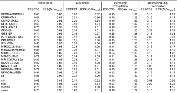
3.2 Significance of scaling patterns extracted from AOGCM simulations

The assumption of a linear relationship between change inTgloband mean local change

of a climate variableV considered is central to pattern scaling. Although it is generally accepted that this assumption holds well for temperature (Mitchell, 2003), it may not be

25

fully valid for other climate variables. The focus of this section is therefore on a com-parison between the different variables rather than between the different AOGCMs. However, values for individual AOGCMs are presented in Table 2.

(21)

GMDD

5, 3533–3572, 2012

J. Heinke et al.

Title Page

Tables Figures

◭ ◮

Back Close

Full Screen / Esc

Discussion

P

a

per

|

Dis

cussion

P

a

per

|

Discussion

P

a

per

|

Discussio

n

P

a

per

|

For ordinary linear square models, such as those fitted to the AOGCM data for pat-tern extraction, the total sum of squares (TSS) equals the sum of explained sum of squares (ESS) and residual sum of squares (RSS). For the pattern extraction, this is described in Eq. (12).

N X

y=1

[∆V(x,m,y)]2=

N X

y=1 [V∗

(x,m)·_∆T_glob(y)]2+

N X

y=1

[∆V(x,m,y)−V∗(x,m)·_∆T_glob(y)]2 (12)

5

Based on this relationship it is possible to evaluate the significance of the extracted patterns by comparing the explained sum of squaresPN

y=1[V

∗

(x,m)·_∆T_glob(y)]2 to the total sum of squaresPN

y=1[∆V(x,m,y)] 2

to provide a measure of explained variance. However, this measure is incomplete without an analysis of how much of the residual

10

sum of squaresPN

y=1[∆V(x,m,y)−V

∗

(x,m)·_∆T_glob(y)]2can be attributed to interannual variability inherent to the climate system. This variability cannot be captured by the linear regression and the separation of the climate signal from the background vari-ability is in fact the basic principle of the pattern-scaling approach. For the analysis of the residual sum of squares the variance of the control run Var_cntrl(x,m) was multiplied

15

with the number of valuesNin the residual sum of squares to obtain an estimate of the total sum of squared interannual variability to be expected in the scenario data.

Because Eq. (12) is valid for every single regression model, the evaluation metrics derived from its terms can be calculated for every model, grid cell, and month. In or-der to facilitate a comparison of the performance for different variables, area-weighted

20

means over all land cells for the different square sums are calculated for each model and month and then again averaged with equal weight.

For the ratio of explained sum of squares to total sum of squares (ESS/TSS), val-ues of 0.81, 0.21, 0.17, and 0.14 are found for temperature, cloudiness, precipitation (increases only), and logarithmic precipitation (decreases only), respectively.

Corre-25

sponding ratios of residual mean of squares to control run variance (RSS/(N·Varcntrl))

(22)

GMDD

5, 3533–3572, 2012

J. Heinke et al.

Title Page

Tables Figures

◭ ◮

Back Close

Full Screen / Esc

Discussion

P

a

per

|

Dis

cussion

P

a

per

|

Discussion

P

a

per

|

Discussio

n

P

a

per

|

comparison of residual variance to the control run variance reveals that most of the unexplained variation can be attributed to the high interannual variability of these vari-ables. This is a clear indication that the derived patterns have a strong significance and can be used in a scenario-building framework such as the one applied here. Even the relatively high value of (RSS/(N·Var_cntrl)) for increasing precipitation (1.30) is not

crit-5

ical if one considers that increases of mean precipitation are usually accompanied by increases in variability. Because a transformation to logarithmic values diminishes this e_ffect, the ratio of residual variance to control run variance is very close to unity (0.98) if it is calculated for increasing logarithmic precipitation. It should be mentioned, however, that precipitation change in the AOGCM simulations is also influenced by factors such

10

as atmospheric aerosol loading. As these e_ffects are not captured by the extracted patterns and therefore contribute to higher (RSS/(N·Varcntrl)) ratios. The ratio of

resid-ual variance to control run variance smaller than unity for temperature means that the residual variation is generally slightly smaller than expected from the interannual vari-ability estimated from the control run. This is an indicator for the strong relationship

15

between local temperature anomalies andTglobanomalies captured by the derived

pat-terns. When using these patterns to predict local temperature anomalies in conjunction with actual∆Tglob(y), the part of interannual variability that can be explained by

inter-annual variability of∆Tglob(y) is included which reduces the residual error. In contrast,

the estimation of control run variance is based on a constant mean climatology and

20

therefore includes the part of variability that is correlated to the variability in∆Tglob(y).

3.3 Applied local anomalies for 1 degree of global warming

The dataset for systematic climate impact assessment presented here is a combina-tion of extracted patterns and the reference time series of temperature, precipitacombina-tion, and cloudiness. While properties of the scaling patterns were discussed in the

pre-25

ceding section, this section explores the actual anomalies by which the scenario time series are shifted. These anomalies were obtained by combining the scaling patterns (representing the anomalies for a 1-degree increase inTglob) with the reference time

(23)

GMDD

5, 3533–3572, 2012

J. Heinke et al.

Title Page

Tables Figures

◭ ◮

Back Close

Full Screen / Esc

Discussion

P

a

per

|

Dis

cussion

P

a

per

|

Discussion

P

a

per

|

Discussio

n

P

a

per

|

series (see Sect. 2.3). The procedure for combining the scaled patterns and the refer-ence time series thereby has the potential to alter the original scaled anomalies if the present climate simulated by the AOGCM disagrees with observations. It is, however, a very general problem how to interpret changes in climatological means when these means are biased. If observed climatology is underestimated the simulated change

5

may underestimate the actual change and vice versa, providing that changes derived from a biased representation of reality are a meaningful source of actual change at all. All assessments that are based on anomalies obtained from AOGCM simulations are confronted with this problem and have to deal with the question whether to use the unchanged absolute anomalies or adjust them according to the biases in the AOGCM’s

10

presentation of actual conditions. In cases where anomalies are combined with obser-vations an adjustment is often inevitable, as a direct use of anomalies can result in violation of valid ranges for some variables (e.g. most variables have a positivity con-straint). In these cases a relative application of anomalies provides a convenient way of accounting for the different base levels in simulations and observations. There are,

15

however, no objective criteria on whether and how to perform this adjustment. Hence, any solution represents a choice that cannot be validated in a meaningful way. Our methodology is no exception from that. It is grounded on common practice found in the impact literature aiming to fulfil the particular requirements of the pattern-scaling approach while minimizing alterations of the original signal. In place of a validation we

20

here complement the presentation of applied anomalies in the end product by a pre-sentation of the alteration of the original scaled anomalies.

For temperature the actual applied anomalies for a 1-degree increase inTglob(Fig. 3)

are identical to the scaling pattern as temperature anomalies are applied as absolute changes (Eq. 4). The spatial distribution of mean annual temperature changes across

25

all AOGCMs exhibits the same overall behaviour as presented and discussed for the CMIP3 ensemble in Solomon et al. (2007). For the considered land area there are no incidents of decreasing local temperature with increasingTglob. Below average warming

(24)

GMDD

5, 3533–3572, 2012

J. Heinke et al.

Title Page

Tables Figures

◭ ◮

Back Close

Full Screen / Esc

Discussion

P

a

per

|

Dis

cussion

P

a

per

|

Discussion

P

a

per

|

Discussio

n

P

a

per

|

inertia of the oceans. Overall, warming on the land surface is above average with a dis-tinct pattern of polar amplification (stronger warming towards higher latitudes). Behind the multi-model annual mean change there is substantial variation in regional temper-ature change both among different AOGCMs and during the course of the year (see Supplement). Disparity among AOGCMs is lower than the projected mean change –

5

i.e. there is some disagreement in the magnitude but not in the direction of change. Seasonality of change is particularly strong in the high northern latitudes and broadly follows the pattern of polar amplification. Hence, the strong average increase projected for these areas does not occur uniformly over the year.

Actual applied anomalies for cloudiness are a mix of cloud cover increases and

de-10

creases (Fig. 4). Strong decreases are found in the Mediterranean, the Middle East, Southern Africa, Southern Australia, Central America, and the Amazon region. In-creases are constrained to the higher northern latitudes and the Horn of Africa. In some areas such as the northernmost latitudes, the Amazon and some parts of Africa varia-tion of projected annual cloud cover change among AOGCMs is high with inter-model

15

standard deviation exceeding the mean change (see Supplement). Significant season-ality in the multi-model mean is limited to a few regions such as the Amazon, Central Asia and North-Eastern Canada only (see Supplement). Regions with pronounced sea-sonality do not always coincide with regions of strong mean change, which indicates a mix of increases and decreases throughout the year that cancel out each other in the

20

annual mean.

Alteration of the absolute signal, averaged over all months and AOGCMs, by the application method described in Sect. 2.3.2 is depicted in the lower panel of Fig. 4. In order to prevent that augmentations of increases and decreases cancel each other out due to their different sign of change, the sign was ignored when computing the

25

alteration of the signal. This results in signal augmentations always being positive and signal attenuations being negative. In most cases the application method augments the original signal, which means that decreases of cloudiness tend to be associated by un-derestimation and increases by overestimation of present-day cloud cover. However, in

(25)

GMDD

5, 3533–3572, 2012

J. Heinke et al.

Title Page

Tables Figures

◭ ◮

Back Close

Full Screen / Esc

Discussion

P

a

per

|

Dis

cussion

P

a

per

|

Discussion

P

a

per

|

Discussio

n

P

a

per

|

most cases the average alteration of the original signal is less than±0.5 %. Significant

alteration of the signal only occurs in Northern Canada, the Amazon, the Middle East and some parts of Africa – all of these regions being characterised by strong mean changes (Fig. 4, upper panel).

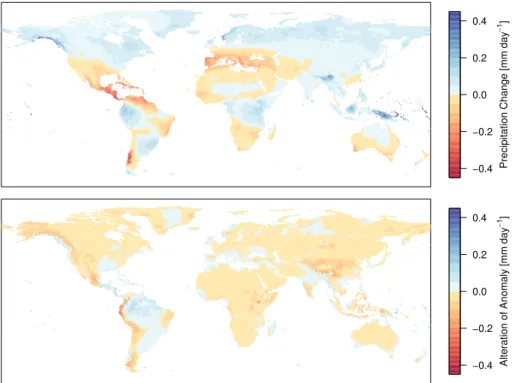
The multi-model mean of annual precipitation change is shown in Fig. 5 (upper

5

panel). As for temperature and cloudiness, precipitation changes are consistent with results presented in Solomon et al. (2007). Significant decreases prevail in the Mediter-ranean, the Middle East, South Africa, Southern Australia, Central America and Patag-onia; increases are projected for the Boreal zone, South and Southeast Asia, East Africa, and parts of South America. For some regions such as the Amazon,

Sub-10

Saharan Africa, and Southeast Asia inter-model standard deviation is high (see Sup-plement), indicating considerable disagreement in the magnitude and in some cases even sign of mean annual precipitation change for the different AOGCMs. Seasonal-ity of change is less pronounced but seems to occur in regions where the inter-model spread is high – i.e. the wet tropics but also in temperate North America and Europe

15

(see Supplement).

Although large biases in the AOGCMs impair the applicability of derived anomalies the alteration of the scaled anomalies by the application method is well controlled and rarely exceeds ±0.05 mm d−1. Significant alterations primarily occur in mountainous

regions (Andes, Rocky Mountains, Himalayas) where the AOGCMs’ coarse spatial

res-20

olution impedes the correct representation of sub-grid orographic effects. In average, our application method attenuates rather than augments the original anomaly, which indicates that AOGCMs tend to overestimate observed precipitation rates. It is not the progressive reduction of the relative anomaly by theλexponent with increasing under-estimation in the AOGCM (Eq. 6) that causes the overall attenuation. The reduction

25

(26)

GMDD

5, 3533–3572, 2012

J. Heinke et al.

Title Page

Tables Figures

◭ ◮

Back Close

Full Screen / Esc

Discussion

P

a

per

|

Dis

cussion

P

a

per

|

Discussion

P

a

per

|

Discussio

n

P

a

per

|

case of underestimation in the AOGCM can become many times bigger than the orig-inal anomaly. With our approach, in contrast, the origorig-inal anomaly is also augmented with increasing underestimation in the AOGCM but reaches a maximum augmentation by a factor of about two for a five-fold underestimation and then declines towards unity for a completely rain-free AOGCM baseline.

5

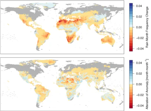
Changes in rain month frequency are rarely analysed and their explicit consider-ation in a pattern-scaling framework is unique. The rain month frequency changes, averaged over all AOGCMs and months, shown in the upper panel of Fig. 6 exhibit both increases and decreases although decreases prevail. As already discussed in Sect. 3.1 changes occur predominately in areas that are already today characterized

10

by intermittent rainfall occurrence while regions such as North America, Northern Eu-rope and Siberia remain unaffected. Regions of strong rain month frequency decrease broadly agree with key regions of decreases in average rainfall but some noteworthy di_fferences exist. Almost entire South America and Australia are, in average, a_ffected by rain month frequency decrease while the picture for change in rainfall amount is

15

much more mixed. In the Mediterranean, Southern Europe is much less affected than it is the case for rainfall amounts while the opposite can be stated for North Africa. In Southern Africa decreases in rain month frequency stretch much further up north along the east coast.

Variation of rain month frequency change among AOGCMs is pronounced but

gen-20

erally follows the pattern of strong decreases (see Supplement). Thus, different models disagree primarily in the magnitude rather than in the direction of change. Seasonal-ity of change is in the same magnitude as the inter-model variation and also exhibits a similar pattern (see Supplement). Hence, decreases in rain month frequency in some months can be very high, while little change occurs in others.

25

Anomalies of rain month frequency are significantly altered by the application method (see Fig. 6, lower panel). Although logit-transformed frequency anomalies are applied as absolute changes (see Sect. 2.3.4) the different reference levels in the AOGCM and the observations result in very different actual frequency anomalies when transformed