www.clim-past.net/10/79/2014/ doi:10.5194/cp-10-79-2014
© Author(s) 2014. CC Attribution 3.0 License.
Climate
of the Past
Evaluating the dominant components of warming in Pliocene
climate simulations
D. J. Hill1,2, A. M. Haywood1, D. J. Lunt3, S. J. Hunter1, F. J. Bragg3, C. Contoux4,5, C. Stepanek6, L. Sohl7, N. A. Rosenbloom8, W.-L. Chan9, Y. Kamae10, Z. Zhang11,12, A. Abe-Ouchi9,13, M. A. Chandler7, A. Jost5, G. Lohmann6, B. L. Otto-Bliesner8, G. Ramstein4, and H. Ueda10
1School of Earth and Environment, University of Leeds, Leeds, UK 2British Geological Survey, Keyworth, Nottingham, UK
3School of Geographical Sciences, University of Bristol, Bristol, UK 4Laboratoire des Sciences du Climat et de l’Environnement, Saclay, France 5Sisyphe, CNRS/UPMC Univ. Paris 06, Paris, France
6Alfred Wegener Institute Helmholtz Centre for Polar and Marine Research, Bremerhaven, Germany 7Columbia University – NASA/GISS, New York, NY, USA
8National Center for Atmospheric Research, Boulder, Colorado, USA
9Atmosphere and Ocean Research Institute, University of Tokyo, Kashiwa, Japan
10Graduate School of Life and Environmental Sciences, University of Tsukuba, Tsukuba, Japan 11UniResearch and Bjerknes Centre for Climate Research, Bergen, Norway
12Nansen-zhu International Research Centre, Institute of Atmospheric Physics, Chinese Academy of Sciences, Beijing, China 13Japan Agency for Marine-Earth Science and Technology, Yokohama, Japan
Correspondence to:D. J. Hill (eardjh@leeds.ac.uk)
Received: 28 February 2013 – Published in Clim. Past Discuss.: 26 March 2013
Revised: 29 November 2013 – Accepted: 2 December 2013 – Published: 15 January 2014
Abstract. The Pliocene Model Intercomparison Project (PlioMIP) is the first coordinated climate model comparison for a warmer palaeoclimate with atmospheric CO2 signifi-cantly higher than pre-industrial concentrations. The simula-tions of the mid-Pliocene warm period show global warming of between 1.8 and 3.6◦C above pre-industrial surface air temperatures, with significant polar amplification. Here we perform energy balance calculations on all eight of the cou-pled ocean–atmosphere simulations within PlioMIP Experi-ment 2 to evaluate the causes of the increased temperatures and differences between the models. In the tropics simulated warming is dominated by greenhouse gas increases, with the cloud component of planetary albedo enhancing the warm-ing in most of the models, but by widely varywarm-ing amounts. The responses to mid-Pliocene climate forcing in the North-ern Hemisphere midlatitudes are substantially different be-tween the climate models, with the only consistent response being a warming due to increased greenhouse gases. In the high latitudes all the energy balance components become
important, but the dominant warming influence comes from the clear sky albedo, only partially offset by the increases in the cooling impact of cloud albedo. This demonstrates the importance of specified ice sheet and high latitude vegeta-tion boundary condivegeta-tions and simulated sea ice and snow albedo feedbacks. The largest components in the overall un-certainty are associated with clouds in the tropics and polar clear sky albedo, particularly in sea ice regions. These simu-lations show that albedo feedbacks, particularly those of sea ice and ice sheets, provide the most significant enhancements to high latitude warming in the Pliocene.
1 Introduction
Table 1.Key model and experimental design parameters for each of the eight PlioMIP Experiment 2 simulations.
GCM Atmospheric Ocean resolution Boundary Ocean Reference resolution (◦lat×◦long×levels) conditions initialization
(◦lat×◦long×levels) employed
CCSM4 0.9×1.25×26 1×1×60 Alternate PRISM3 Rosenbloom et (anomaly) al. (2013)
COSMOS 3.75×3.75×19 3×1.8×40 Preferred PRISM3 Stepanek and (anomaly) Lohmann (2012)
GISS-E2-R 2×2.5×40 1×1.25×32 Preferred PRISM3 Chandler et al. (2013)
HadCM3 2.5×3.75×19 1.25×1.25×20 Alternate PRISM2 Bragg et al. mPWP control (2012)
IPSLCM5A 3.75×1.9×39 0.5–2×2×31 Alternate Pre-industrial Contoux et al. control (2012)
MIROC4m 2.8×2.8×20 0.5–1.4×1.4×43 Preferred PRISM3 Chan et al. (2011)
MRI-CGCM 2.3 2.8×2.8×30 0.5–2×2.5×23 Alternate PRISM3 Kamae and (anomaly) Ueda (2012) NorESM-L 3.75×3.75×26 3×3×30 Alternate Levitus Zhang et al.
(2012)
was the last period of Earth history with similar to modern at-mospheric CO2concentrations (Kürschner et al., 1996; Seki et al., 2010; Pagani et al., 2010; Bartoli et al., 2011). These were associated with elevated global temperatures in both the ocean (Dowsett et al., 2012) and on land (Salzmann et al., 2013). As the last period of global warmth before the climate transition into the bipolar ice age cycles of the Pleistocene, the mid-Pliocene warm period (mPWP) has been a target for both palaeoenvironmental data acquisition and palaeo-climate modelling over a number of years (Dowsett et al., 1992; Chandler et al., 1994; Haywood et al., 2009; Dowsett et al., 2010). Although a number of different general circula-tion models (GCMs) have been used to simulate Pliocene cli-mates (Chandler et al., 1994; Sloan et al., 1996; Haywood et al., 2000, 2009; Dowsett et al., 2011), it is only recently that a coordinated multi-model experiment has been initiated, with standardized design for mid-Pliocene simulations (Haywood et al., 2010, 2011).
The Pliocene Model Intercomparison Project (PlioMIP) represents the first coordinated multi-model experiment to simulate a warmer than modern palaeoclimate, with high at-mospheric CO2 concentrations (405 ppmv). It has recently been added to the Paleoclimate Model Intercomparison Project (PMIP; Hill et al., 2012) and the first phase, in-corporating two simulations, completed. This paper focuses on PlioMIP Experiment 2, designed for coupled ocean– atmosphere GCMs (Haywood et al., 2011). Although, many of the large-scale features of the simulated Pliocene climate have been well documented (Dowsett et al., 2012; Haywood et al., 2013; Zhang et al., 2013, 2013a,b; Salzmann et al., 2013), the causes of the simulated changes and differences
between the simulations have not been extensively explored prior to this study. In this paper the energy balance of the PlioMIP Experiment 2 simulations are analysed in order to understand the causes of Pliocene atmospheric warming and the latitudinal distribution of increased surface air tempera-tures. This analysis allows us to analyse the causes of the warming, both directly through the simulated energy balance components and through examination of Earth system com-ponent changes that are driving these. It is also important when discrepancies with available proxy reconstructions of Pliocene warming are considered (Salzmann et al., 2013).
2 Participating models
Table 2.The climate sensitivity and global mean annual surface air temperature warming of each of the models with simulations in the PlioMIP Experiment 2 ensemble. Climate sensitivity is the equilibrium global warming for a doubling of atmospheric CO2– the values quoted here are a general value for each model and do not refer to the particular set-up and initialization procedures used for PlioMIP.
GCM Climate Mean annual sensitivity mPWP SAT
(◦C) warming (◦C) CCSM4 3.2 1.86 COSMOS 4.1 3.60 GISS-E2-R 2.7 2.24 HadCM3 3.1 3.27 IPSLCM5A 3.4 2.03 MIROC4m 4.1 3.46 MRI-CGCM 2.3 3.2 1.84 NorESM-L 3.1 3.27
3 PlioMIP Experiment 2
PlioMIP uses the latest iteration of the PRISM (Pliocene Re-search, Interpretation and Synoptic Mapping) mid-Pliocene palaeoenvironmental reconstruction, PRISM3 (Dowsett et al., 2010), as the basis for the imposed model boundary conditions. This reconstruction represents the peak averaged (Dowsett and Poore, 1991) warm climate of the mid-Pliocene warm period (mPWP; 3.246–3.025 Ma; Dowsett et al., 2010) in the middle of the Piacenzian Stage. It incorporates sea surface temperatures, bottom water temperatures (Dowsett et al., 2009), vegetation (Salzmann et al., 2008), ice sheets (Hill et al., 2007, 2010), orography (Sohl et al., 2009) and a global land-sea mask equivalent to 25 m of sea level rise. The vegetation, ice sheets and orographic reconstructions are all required as boundary conditions within the models, although they must be translated onto the resolution of each individ-ual model. Vegetation was reconstructed using the BIOME4 classification scheme (Kaplan, 2001) and must therefore be translated onto the vegetation scheme used by each model.
Although as part of PlioMIP a standard experimental de-sign was implemented, it was appreciated that not all of the modelling groups would be able to perform the ideal mPWP experiment. As such, alternate boundary conditions were specified for those models that could not effectively change the land-sea mask from the present-day configuration. This meant that the ocean advance specified in low-lying coastal regions and West Antarctica as well as the filling of Hudson Bay were not included in some of the simulations (Table 1). Furthermore a choice was given concerning the initial state of the ocean between a specification of the PRISM3 three-dimensional ocean temperatures (Dowsett et al., 2009) and initialization with the same ocean temperatures as the pre-industrial control simulation (Haywood et al., 2011).
4 PlioMIP Experiment 2 global warming
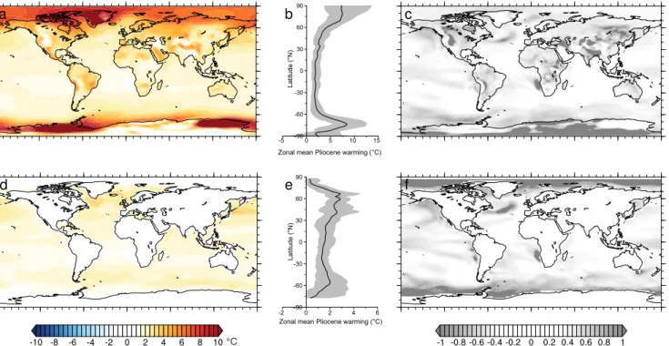
Overall the PlioMIP models simulate mPWP annual mean global surface air temperature (SAT) increases of 1.8–3.6◦C (Table 2). Tropical temperatures increased by only 1.0– 3.1◦C, while in the Arctic surface air temperatures increased by 3.5–13.2◦C (Fig. 1). Sea surface temperatures (SSTs) fol-low a similar pattern, but with a reduced magnitude of global warming and significantly greater warming in the North Pa-cific (Fig. 1d). The patterns of warming in the northern mid-latitudes and southern high mid-latitudes are much more variable between the different models. Relative variation between the models is largest in the North Atlantic, midlatitude mountain regions and central Antarctica for SATs (Fig. 1c) and in the North Atlantic, North Pacific and sea ice areas of the Arctic and Southern oceans for SSTs (Fig. 1f).
The warming of the PlioMIP simulations is accompanied by increased precipitation (Haywood et al., 2013) and mon-soonal activity (Zhang et al., 2013) and reductions in sea ice (Clark et al., 2013), although the Atlantic Meridional Overturning Circulation shows little response (Zhang et al., 2013b). Global mean temperature response (Table 2), as well as polar amplification (Salzmann et al., 2013), do not show a strong correlation to either the use of preferred or alter-nate boundary conditions or to the initial conditions of the ocean. Although land-sea masks vary between the different models in the Hudson Bay and West Antarctic region, they do not show the largest relative variance, suggesting that the alternatives used in PlioMIP Experiment 2 do not introduce significant biases.
5 Energy balance approach
Energy balance analyses have been used in many palaeocli-mate simulations and ensembles to understand the simulated temperature changes (e.g. Donnadieu et al., 2006; Murakami et al., 2008). The results from each of the GCMs can be bro-ken down in to the various components in the energy balance of each individual simulation. The approach taken builds on the energy balance modelling of Heinemann et al. (2009) and Lunt et al. (2012), where globally averaged temperatures are approximated using planetary albedoαand the effective longwave emissivityε.
S0
4 (1−α)=ε σ T 4,
(1) whereS0 is the total solar irradiance (1367 Wm−2) and σ is the Stefan–Boltzmann constant (5.67×10⁻⁸Wm−2K−4). Planetary albedo is the ratio of outgoing (↑) to incoming (↓) shortwave radiation at the top of the atmosphere (TOA) and effective longwave emissivity the ratio of TOA to surface (SURF) upward longwave radiation,
α= SW
↑
TOA
SW↓TOA
, ε = LW
↑
TOA
LW↑SURF
a b c
e f
d
°C
Fig. 1.Multi-model mean PlioMIP Experiment 2 warming between mid-Pliocene and pre-industrial simulations.(a)Annual mean surface air temperature (SAT) warming,(b)zonal mean SAT warming (solid line), with shading showing the range of model simulations, and (c)relative variance between the PlioMIP Experiment 2 simulations (σ/1SAT).(d)Annual mean sea surface temperature (SST) warming, (e)zonal mean SST warming and(f)relative variance of SSTs.
This can be expanded to approximate the one dimensional, zonally averaged temperatures at each latitude of the model grid by including a component for the implied net meridional heat transport divergence (H).
SW↓TOA(1−α)+H =ε σ T4, (3) where
H = −SW↓TOA−SWTOA↑ −LW↑TOA. (4) Thus the temperature at each latitude in a GCM experiment is given by
T = SW
↓
TOA(1−α)−H ε σ
!1/4
≡T (ε, α, H ). (5)
By applying the notation of Lunt et al. (2012) to denote the pre-industrial control experiment as a second experiment rep-resented by an apostrophe, the Pliocene surface air tempera-ture warming (1T) can be calculated by
1T =T (ε, α, H )−T (ε′, α′, H′). (6) Due to their small changes relative to their absolute values, Pliocene warming can be approximated by a linear combi-nation of changes in emissivity (1Tε), albedo (1Tα) and heat transport (1TH). However, these components can be
further broken down into the changes in the impact of at-mospheric greenhouse gases (1Tggε), clouds (via impacts on both emissivity, 1Tcε, and albedo, 1Tcα; see Sect. 6 for discussion) and clear sky albedo (1Tcsα; generally dom-inated by changes in surface albedo, but including atmo-spheric absorption and scattering components). In experi-ments and latitudes where changes in topography occur be-tween the Pliocene and pre-industrial times, the impact of these changes in surface altitude (1Ttopo) must also be ac-counted for.
1T ≈1Tggε+1Tcε+1Tcα+1Tcsα+1TH+1Ttopo (7) Each of these components can be calculated from various combinations of Pliocene and pre-industrial albedos, emis-sivities and implied heat transports, although to differentiate between cloud and clear sky components some must be cal-culated in the clear sky case (denoted with a subscript cs). 1Tggε =T (εcs, α, H )−T (ε′cs, α, H )−1Ttopo (8) 1Tcε =(T (ε, α, H )−T (εcs, α, H ))
− T (ε′, α, H )−T εcs′ , α, H
(9) 1Tcα =(T (ε, α, H )−T (ε, αcs, H ))
− T (ε, α′, H )−T ε, αcs′ , H
(10) 1Tcsα =T (ε, αcs, H )−T ε, αcs′ , H
Changing the topography within a climate model can have many effects on the energy balance of the model, including changing circulation patterns, heat transport, surface condi-tions, cloud formation, storm generation, etc. Most of these features cannot be properly quantified without performing further simulations. However, a simple lapse rate correc-tion will remove the direct impact on surface temperatures of changing the height of the surface. Although lapse rates vary over time and space, the impact of changing the topog-raphy in the Pliocene simulations (1Ttopo) can be approxi-mated by multiplying the change in topography (1h) by a constant atmospheric lapse rate (γ≈5.5 K km−1; Yang and Smith, 1985).
1Ttopo =1h·γ (13)
6 Treatment of clouds within the energy balance calculations
The energy balance calculations presented here split the plan-etary albedo and emissivity impacts into a component due to clouds and a clear sky one. In order to do this the clear sky radiation fluxes, which are the radiation fluxes that would have occurred had there not been any clouds, are used within the calculations. The cloud components are then the global temperature change due to the impact of clouds on planetary albedo and emissivity. If all else in the climate system re-mained the same except for the surface albedo then the clear sky albedo would show a change in temperature, but so also would the cloud albedo. This is because the impact of iden-tical clouds on the total planetary albedo have changed due to the surface which they are covering being different. Simi-larly an increase in highly reflective cloud types would have a greater impact on temperature over the dark oceans than over a high albedo land surface.
A more thorough methodology for calculating the cloud and clear sky components would be to incorporate cloudi-ness into the calculations and thereby remove the reliance of cloud impact on the surface conditions. This requires an un-derstanding of the impact of different modelled cloud types on the energy balance and, as we are considering a multi-model ensemble, the consistent application of this across all the simulations within the ensemble. Total cloud fractions are produced by each model, but these use different overlap functions, all of which are simplifications of the observed de-pendencies of cloud overlap on atmospheric dynamics (Wang and Dessler, 2006; Naud et al., 2008). Therefore, the total cloud fractions of the models are not only incomparable, but may also not be the best representation of cloud impacts on energy balance.
The impact of using the pragmatic methodology outlined above can be approximated using the surface downward shortwave radiation to approximate the impact of clouds. Figure 2 shows the albedo components of Pliocene warming in the HadCM3 model, using both this approximation and the
Fig. 2.Comparison of the impact on Pliocene warming of the com-ponents of planetary albedo under different formulations for the HadCM3 model. The grey lines are the formulations presented in this Sect. 5, while the black lines represent an altered calculation of the albedo components approximating the impact of clouds us-ing the difference between the incomus-ing radiation at the top of the atmosphere and the modelled downward shortwave radiation at the surface.
methodology outlined in Sect. 5. Although using the outlined energy balance approach produces greater magnitudes of im-pacts from clear sky and cloud albedo, as would be expected, the overall structure and the conclusions that would be drawn from these calculations remain.
7 Energy balance results for individual simulations
Antarctic continents, from prescribed changes to the Antarc-tic ice sheets.
8 PlioMIP Experiment 2 energy balance
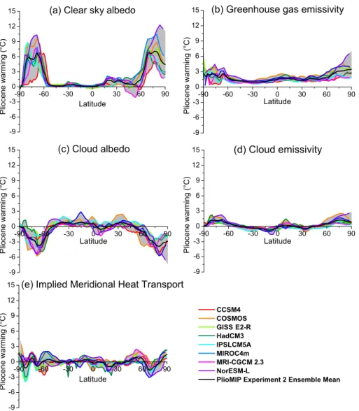
In order to evaluate the simulation of warm climates of the Pliocene in general, a simple mean of the energy bal-ance components from each of the individual simulations within the PlioMIP Experiment ensemble has been per-formed. When combined with the range of values within the ensemble this allows an assessment of the general cause of warming within the PlioMIP simulations and the robustness of any conclusion that can be drawn. Figure 4 shows the ensemble mean of the various energy balance components along with the range from the eight simulations, while Fig. 5 shows the individual energy balance components for each of the PlioMIP simulations.
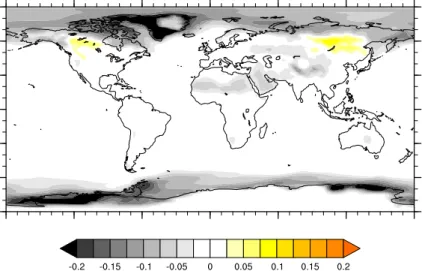
Clear sky albedo includes contributions from surface albedo changes and atmospheric absorption and scattering. The latter could become important, even in models with no mechanisms for changing atmospheric transparency, as atmospheric thickness can increase due to changes in sur-face altitude. In the PlioMIP simulations clear sky albedo shows little contribution to warming in the tropics and South-ern Hemisphere midlatitudes. In the NorthSouth-ern Hemisphere midlatitudes most models show a warming due to clear sky albedo, apart from the MRI-CGCM 2.3 simulation that shows a cooling (Fig. 5a). In the polar regions, all the simu-lations show a strong warming signal from clear sky albedo, although the range in the magnitude of this warming is large. Changes in clear sky albedo mostly reflect changes on Earth’s surface. Vegetation, snow and ice (both terrestrial ice masses and sea ice) are generally the main contributors to these changes. The warming found in the Northern Hemi-sphere, from 15–60◦N is largely being driven by changes in the vegetation boundary conditions, particularly over the Sa-hara, Arabia and central Asia (Fig. 6). In the Arctic, warm-ing due to clear sky albedo is primary driven by changes in ice sheet boundary conditions (reduced Greenland Ice Sheet) and changes in the predicted sea ice, but also by the pole-ward shift of the Arctic tree line (Salzmann et al., 2008). In the Southern Ocean and Antarctica the warming due to clear sky albedo has a double peak in most models, reflect-ing a reduction in the simulated Southern Ocean sea ice and a reduction in the prescribed Antarctic Ice Sheet (Fig. 7). Most models show reductions in sea ice coverage across the whole range of latitudes in which sea ice is modelled, except for the highest Northern Hemisphere latitudes and in CCSM close to Antarctica (Fig. 7c). The simulated changes in total cloud are relatively small and inconsistent between the mod-els (Fig. 7e), so do not appear to introduce systematic biases. All the simulations show a warming due to greenhouse gas emissivity of around 1–2◦C. These impacts are largely con-stant across latitudes, but with a slight polar amplification,
Fig. 4.Summary of the PlioMIP Experiment 2 energy balance anal-ysis. Solid line shows the multi-model mean warming for each com-ponent, with the associated shading representing the range. These values have been interpolated onto a 1◦latitude grid for compari-son purposes.
especially in the Arctic (Fig. 5b). This is consistent with the prescribed increases in CO2 (at 405 ppm for the mid-Pliocene, as opposed to 280 ppm in the pre-industrial sim-ulations). The amplified high-latitude response is due to in-creases in the atmospheric water vapour predicted by the models. Differences in the simulation of this water vapour increase between different models explain why the range of temperature increases due to greenhouse gas warming is much higher in the polar regions.
The changes in the impact of clouds on planetary albedo are small in the tropics and midlatitudes. Different models seem to produce significantly different responses making the signal particularly noisy (Fig. 5c). However, the multi-model mean cloud albedo impact on warming appears to reflect some of the large-scale features of the PlioMIP simulations (Haywood et al., 2013). Between the Equator and∼45◦there is a general warming due to a reduction in the impact of cloud albedo, interrupted by a cooling in the Northern Hemisphere tropics. This cooling is due to an increase in cloud cover re-sulting from a northward shift of the Inter-Tropical Conver-gence Zone (Kamae et al., 2011). In the high latitudes the increased impact of clouds on planetary albedo, partly due to changes in the underlying surface albedo, leads to a signif-icant cooling, peaking at between 3 and 6◦C in both
hemi-spheres. Cloud emissivity shows a similar pattern of impacts, but in the opposite direction. However, the response is gen-erally of a smaller magnitude (Fig. 5d).
Fig. 5.Breakdown of the energy balance components,(a)clear sky albedo,(b)greenhouse gas emissivity,(c) cloud albedo,(d)cloud emissivity and(e)implied meridional heat transport. Solid black line shows the multi-model mean, range is shown by the grey shading and each of the individual model results is shown by the coloured solid lines.
one region where all of the simulations show a temperature change of the same direction suggests that the only robust conclusion that can be drawn about heat transport is a re-duction of overall transport into the Arctic (Fig. 5e). This would be an expected result of reduced thermal gradients due to polar amplification in the Arctic region under climate warming. These energy balance calculations support analy-sis of the Atlantic Meridional Overturning Circulation in the PlioMIP ensemble, which shows that there is little change in the northward heat transport in the North Atlantic (Zhang et al., 2013b). This calls into question the role of ocean heat transport in the general warming of the mid-Pliocene. How-ever, it may be important in the Pliocene variability of sea surface temperatures, which is particularly high in the North Atlantic (Dowsett et al., 2012).
9 Conclusions
Fig. 6.Spatial distribution of multi-model mean changes in the clear sky albedo between mid-Pliocene and pre-industrial simulations. This primarily shows changes due to specified vegetation and global ice sheets and modelled sea ice and snow cover, although it includes an atmospheric component. Greyscale shows reductions in albedo, generally associated with warming and yellow shading indicates increases in albedo that would generally cause a reduction in surface air temperature. Increases in albedo closely follow the northward expansion of grassland imposed on the simulations (Haywood et al., 2010).
hampered by differing experimental designs (Haywood et al., 2009). For the first time a robust analysis of the causes of warming in Pliocene climate models is possible.
Energy balance calculations show that the tropical warm-ing seen in all the models is primarily caused by green-house gas emissivity, with specified increases in atmospheric CO2 concentration being the most important factor. Along with different sensitivity to the imposed CO2concentrations, changes in warming due to the cloud impact on planetary albedo drive differences between the models in the tropics. At polar latitudes all the energy balance components become important, but clear sky albedo is the dominant driver of the high levels of warming and polar amplification. This is largely due to reductions in the specified ice sheets and sim-ulated sea ice, but in the Northern Hemisphere also reflects a northward shift in the treeline. The models show a very different response in the midlatitudes of the Northern Hemi-sphere, with large uncertainties in the relative contributions of the different energy balance components. This is partic-ularly true for the North Atlantic and Kuroshio Current re-gions, where intermodel variability is highest and warming is simulated very differently (Haywood et al., 2013). A more complete picture of these currents, their strength and variabil-ity within the Pliocene, would enable a much better analysis of the skill of the models in these key regions.
Atmospheric CO2concentrations remain a significant un-certainty in Pliocene climate, with different proxy techniques producing values between pre-industrial levels and double pre-industrial levels (Kürschner et al., 1996; Seki et al., 2010; Pagani et al., 2010; Bartoli et al., 2011). As tropical warming is largely driven by this factor, simulations with accurate rep-resentation of low latitude clouds could provide some new
insight into the levels of CO2 required to produce Pliocene climates (for example in a similar way to Lunt et al., 2012, for the Eocene). Alternatively, accurate reconstructions of sur-face temperatures and atmospheric CO2in combination with modelling studies could reveal the extent of changes to trop-ical cloud cover in the warmer Pliocene world.
(a) Warming impact of clear sky albedo
(b) Surface albedo change
(c) Sea ice change
(d) Imposed snow free albedo change
(e) Change in modelled total cloud
Fig. 7.Zonal mean of a series of factors that contribute to the clear sky albedo and its impact on Pliocene warming.(a)The total Pliocene warming and the clear sky albedo component of this (black and green respectively; see Fig. 4).(b)Total zonal surface albedo change in each of the 8 models.(c)Zonal mean sea ice percent coverage in the models, solid line is the Pliocene total and the dashed line is the change between Pliocene and pre-industrial experiments.(d)Imposed snow free albedo change, as calculated from the observed and reconstructed Pliocene mega-biomes, which include vegetation and ice sheet changes (Salzmann et al., 2008; Haywood et al., 2010).(e)Change in modelled total percent cloud cover for each model. These are calculated by each of the models using their own algorithm and cloud parameterizations, so are indicative rather than directly comparable.
Acknowledgements. D. J. Hill acknowledges the Leverhulme Trust
for the award of an Early Career Fellowship and the National Centre for Atmospheric Science and the British Geological Survey for financial support. A. M. Haywood and S. J. Hunter acknowledge that the research leading to these results has received funding from the European Research Council under the European Union’s Seventh Framework Programme (FP7/2007-2013)/ERC grant agreement no. 278636. A. M. Haywood acknowledges funding received from the Natural Environment Research Council (NERC Grant NE/I016287/1, and NE/G009112/1 along with D. J. Lunt). D. J. Lunt and F. J. Bragg acknowledge NERC grant NE/H006273/1. D. J. Lunt acknowledges Research Councils UK for the award of an RCUK fellowship and the Leverhulme Trust for the award of a Phillip Leverhulme Prize. The HadCM3
thank the Japan Society for the Promotion of Science for financial support and R. Ohgaito for advice on setting up the MIROC4m experiments on the Earth Simulator, JAMSTEC. The source code of the MRI model is provided by S. Yukimoto, O. Arakawa, and A. Kitoh of the Meteorological Research Institute, Japan. Z. Zhang acknowledges that the development of NorESM-L was supported by the Earth System Modelling (ESM) project funded by Statoil, Norway. Two anonymous reviewers are thanked for the improvements to the manuscript they inspired. Aisling Dolan is acknowledged for a beautiful title for this paper.
Edited by: C. Brierley
References
Bartoli, G., Hönisch, B., and Zeebe, R. E.: Atmospheric CO2 decline during the Pliocene intensification of North-ern Hemisphere glaciations. Paleoceanography, 26, PA4213, doi:10.1029/2010PA002055, 2011.
Bragg, F. J., Lunt, D. J., and Haywood, A. M.: Mid-Pliocene cli-mate modelled using the UK Hadley Centre Model: PlioMIP Experiments 1 and 2, Geosci. Model Dev., 5, 1109–1125, doi:10.5194/gmd-5-1109-2012, 2012.
Chan, W.-L., Abe-Ouchi, A., and Ohgaito, R.: Simulating the mid-Pliocene climate with the MIROC general circulation model: experimental design and initial results, Geosci. Model Dev., 4, 1035–1049, doi:10.5194/gmd-4-1035-2011, 2011.
Chandler, M., Rind, D., and Thompson, R.: Joint investigations of the middle Pliocene climate II: GISS GCM Northern Hemisphere results, Global Planet. Change, 9, 197–219, 1994.
Chandler, M. A., Sohl, L. E., Jonas, J. A., Dowsett, H. J., and Kelley, M.: Simulations of the mid-Pliocene Warm Period using two ver-sions of the NASA/GISS ModelE2-R Coupled Model, Geosci. Model Dev., 6, 517–531, doi:10.5194/gmd-6-517-2013, 2013. Clark, N. A., Williams, M., Hill, D. J., Quilty, P., Smellie, J.,
Za-lasiewicz, J., Leng, M., and Ellis, M.: Fossil proxies of near-shore sea surface temperature and seasonality from the late Neogene Antarctic shelf, Naturwissenschaften, 100, 699–722, 2013. Contoux, C., Ramstein, G., and Jost, A.: Modelling the
mid-Pliocene Warm Period climate with the IPSL coupled model and its atmospheric component LMDZ5A, Geosci. Model Dev., 5, 903–917, doi:10.5194/gmd-5-903-2012, 2012.
Conway, T. J., Lang, P. M., and Masarie, K. A.: Atmospheric carbon dioxide dry air mole fractions from the NOAA ESRL Carbon Cy-cle Cooperative Global Air Sampling Network, 1968–2011, Ver-sion: 2012-08-15, available at: ftp://ftp.cmdl.noaa.gov/ccg/co2/ flask/event/ (last access: 27 February 2013), 2012.
Donnadieu, Y., Pierrehumbert, R., Jacob, R., and Fluteau, F.: Mod-elling the primary control of paleogeography on Cretaceous cli-mate, Earth Planet. Sc. Lett., 248, 426–437, 2006.
Dowsett, H. J. and Poore, R. Z.: Pliocene sea surface temperatures of the North Atlantic Ocean at 3.0 Ma, Quaternary Sci. Rev., 10, 189–204, 1991.
Dowsett, H. J., Cronin, T. M., Poore, R. Z., Thompson, R. S., What-ley, R. C., and Wood, A. M.: Micropaleontological evidence for increased meridional heat transport in the North Atlantic Ocean during the Pliocene, Science, 258, 1133–1135, 1992.
Dowsett, H. J., Robinson, M. M., and Foley, K. M.: Pliocene three-dimensional global ocean temperature reconstruction, Clim. Past, 5, 769–783, doi:10.5194/cp-5-769-2009, 2009.
Dowsett, H. J., Robinson, M., Haywood, A. M., Salzmann, U., Hill, D. J., Sohl, L., Chandler, M. A., Williams, M., Foley, K., and Stoll, D.: The PRISM3D Paleoenvironmental Reconstruc-tion, Stratigraphy, 7, 123–139, 2010.
Dowsett, H. J., Haywood, A. M., Valdes, P. J., Robinson, M. M., Lunt, D. J., Hill, D. J., Stoll, D. K., and Foley, K. M.: Sea surface temperatures of the mid-Piacenzian Warm Period: A comparison of PRISM3 and HadCM3, Palaeogeogr. Palaeocl., 309, 83–91, 2011.
Dowsett, H. J., Robinson, M. M., Haywood, A. M., Hill, D. J., Dolan, A. M., Stoll, D. K., Chan, W. L., Abe-Ouchi, A., Chan-dler, M. A., Rosenbloom, N. A., Otto-Bleisner, B. L., Bragg, F. J., Lunt, D. J., Foley, K. M., and Riesselman, C. R.: Assessing confidence in Pliocene sea surface temperatures to evaluate pre-dictive models, Nat. Clim. Change, 2, 365–371, 2012.
Haywood, A. M., Valdes, P. J., and Sellwood, B. W.: Global scale palaeoclimate reconstruction of the middle Pliocene climate us-ing the UKMO GCM: initial results, Global Planet. Change, 25, 239–256, 2000.
Haywood, A. M., Chandler, M. A., Valdes, P. J., Salzmann, U., Lunt, D. J., and Dowsett, H. J.: Comparison of mid-Pliocene cli-mate predictions produced by the HadAM3 and GCMAM3 Gen-eral Circulation Models, Global Planet. Change, 66, 208–224, doi:10.1016/j.gloplacha.2008.12.014, 2009.
Haywood, A. M., Dowsett, H. J., Otto-Bliesner, B., Chandler, M. A., Dolan, A. M., Hill, D. J., Lunt, D. J., Robinson, M. M., Rosen-bloom, N., Salzmann, U., and Sohl, L. E.: Pliocene Model Inter-comparison Project (PlioMIP): experimental design and bound-ary conditions (Experiment 1), Geosci. Model Dev., 3, 227–242, doi:10.5194/gmd-3-227-2010, 2010.
Haywood, A. M., Dowsett, H. J., Robinson, M. M., Stoll, D. K., Dolan, A. M., Lunt, D. J., Otto-Bliesner, B., and Chandler, M. A.: Pliocene Model Intercomparison Project (PlioMIP): experi-mental design and boundary conditions (Experiment 2), Geosci. Model Dev., 4, 571–577, doi:10.5194/gmd-4-571-2011, 2011. Haywood, A. M., Hill, D. J., Dolan, A. M., Otto-Bliesner, B. L.,
Bragg, F., Chan, W.-L., Chandler, M. A., Contoux, C., Dowsett, H. J., Jost, A., Kamae, Y., Lohmann, G., Lunt, D. J., Abe-Ouchi, A., Pickering, S. J., Ramstein, G., Rosenbloom, N. A., Salz-mann, U., Sohl, L., Stepanek, C., Ueda, H., Yan, Q., and Zhang, Z.: Large-scale features of Pliocene climate: results from the Pliocene Model Intercomparison Project, Clim. Past, 9, 191–209, doi:10.5194/cp-9-191-2013, 2013.
Heinemann, M., Jungclaus, J. H., and Marotzke, J.: Warm Pale-ocene/Eocene climate as simulated in ECHAM5/MPI-OM, Clim. Past, 5, 785–802, doi:10.5194/cp-5-785-2009, 2009.
Hill, D. J., Dolan, A. M., Haywood, A. M., Hunter, S. J., and Stoll, D. K.: Sensitivity of the Greenland Ice Sheet to Pliocene sea sur-face temperatures, Stratigraphy, 7, 111–122, 2010.
Hill, D. J., Haywood, A. M., Lunt, D. J., Otto-Bliesner, B. L., Har-rison, S. P., and Braconnot, P.: Paleoclimate modelling: an inte-grated component of climate change science, PAGES Newsletter, 20, 103, 2012.
Kamae, Y. and Ueda, H.: Mid-Pliocene global climate simula-tion with MRI-CGCM2.3: set-up and initial results of PlioMIP Experiments 1 and 2, Geosci. Model Dev., 5, 793–808, doi:10.5194/gmd-5-793-2012, 2012.
Kamae, Y., Ueda, H., and Kitoh, A.: Hadley and Walker circulations in the mid-Pliocene Warm Period simulated by an Atmospheric General Circulation Model, J. Meteorol. Soc. Jpn., 89, 475–493, 2011.
Kaplan, J. O.: Geophysical applications of vegetation modeling, PhD thesis, Lund University, Lund, 2001.
Kürschner, W. M., van der Burgh, J., Visscher, H., and Dilcher, D. L.: Oak leaves as biosensors of late Neogene and early Pleistocene paleoatmospheric CO2 concentrations, Mar. Mi-cropalaeontol., 27, 299–312, 1996.
Lunt, D. J., Haywood, A. M., Schmidt, G. A., Salzmann, U., Valdes, P. J., and Dowsett, H. J.: Earth system sensitivity inferred from Pliocene modelling and data, Nat. Geosci., 3, 60–64, 2010. Lunt, D. J., Dunkley Jones, T., Heinemann, M., Huber, M.,
LeGrande, A., Winguth, A., Loptson, C., Marotzke, J., Roberts, C. D., Tindall, J., Valdes, P., and Winguth, C.: A model– data comparison for a multi-model ensemble of early Eocene atmosphere–ocean simulations: EoMIP, Clim. Past, 8, 1717– 1736, doi:10.5194/cp-8-1717-2012, 2012.
Murakami, S., Ohgaito, R., Abe-Ouchi, A., Crucifix, M., and Otto-Bliesner, B. L.: Global-scale energy and freshwater balance in glacial climate: A comparison of three PMIP2 LGM simulations, J. Climate, 21, 5008–5033, 2008.
Naud, C. M., Del Genio, A., Mace, G. G., Benson, S., Clothiaux, E. E., and Kollias, P.: Impact of dynamics and atmospheric state on cloud vertical overlap, J. Climate, 21, 1758–1770, 2008. Pagani, M., Liu, Z. H., LaRiviere, J., and Ravelo, A. C.: High
Earth-system climate sensitivity determined from Pliocene car-bon dioxide concentrations, Nat. Geosci., 3, 27–30, 2010. Raymo, M. E., Grant, B., Horowitz, M., and Rau, G. H.:
Mid-Pliocene warmth: Stronger greenhouse and stronger conveyor, Mar. Micropalaeontol., 27, 313–326, 1996.
Rosenbloom, N. A., Otto-Bliesner, B. L., Brady, E. C., and Lawrence, P. J.: Simulating the mid-Pliocene Warm Period with the CCSM4 model, Geosci. Model Dev., 6, 549–561, doi:10.5194/gmd-6-549-2013, 2013.
Salzmann, U., Haywood, A. M., Lunt, D. J., Valdes, P. J., and Hill, D. J.: A new global biome reconstruction and data-model comparison for the Middle Pliocene, Global Ecol. Biogeogr., 17, 432–447, 2008.
Salzmann, U., Dolan, A. M., Haywood, A. M., Chan, W.-L., Voss, J., Hill, D. J., Abe-Ouchi, A., Otto-Bliesner, B. L., Bragg, F. J., Chandler, M. A., Contoux, C., Dowsett, H. J., Jost, A., Ka-mae, Y., Lohmann, G., Lunt, D. J., Pickering, S. J., Pound, M. J., Ramstein, G., Rosenbloom, N. A., Sohl, L., Stepanek, C., Ueda, H., and Zhang, Z.: Challenges in quantifying Pliocene terrestrial warming revealed by data-model discord, Nat. Clim. Change, 3, 969–974, 2013.
Seki, O., Foster, G. L., Schmidt, D. N., Mackensen, A., Kawa-mura, K., and Pancost, R. D.: Alkenone and boron based PliocenepCO2records, Earth Planet. Sc. Lett., 292, 201–211, doi:10.1016/j.epsl.2010.01.037, 2010.
Sloan, L. C., Crowley, T. J., and Pollard, D.: Modeling of middle Pliocene climate with the NCAR GENESIS general circulation model, Mar. Micropaleontol., 27, 51–61, 1996.
Sohl, L. E., Chandler, M. A., Schmunk, R. B., Mankoff, K., Jonas, J. A., Foley, K. M., and Dowsett, H. J.: PRISM3/GISS topographic reconstruction, US Geol. Surv. Data Series 419, US Geological Survey, Reston, VA, USA, 2009.
Stepanek, C. and Lohmann, G.: Modelling mid-Pliocene cli-mate with COSMOS, Geosci. Model Dev., 5, 1221–1243, doi:10.5194/gmd-5-1221-2012, 2012.
Wang, L. and Dessler, A. E.: Instantaneous cloud overlap statistics in the tropical area revealed by ICESat/GLAS data, Geophys. Res. Lett., 33, L15804, doi:10.1029/2005GL024350, 2006. Yang, S.-K. and Smith, G.L.: Further studies on atmospheric lapse
rate regimes, J. Atmos. Sci., 42, 961–965, 1985.
Zhang, R., Yan, Q., Zhang, Z. S., Jiang, D., Otto-Bliesner, B. L., Haywood, A. M., Hill, D. J., Dolan, A. M., Stepanek, C., Lohmann, G., Contoux, C., Bragg, F., Chan, W.-L., Chandler, M. A., Jost, A., Kamae, Y., Abe-Ouchi, A., Ramstein, G., Rosen-bloom, N. A., Sohl, L., and Ueda, H.: Mid-Pliocene East Asian monsoon climate simulated in the PlioMIP, Clim. Past, 9, 2085– 2099, doi:10.5194/cp-9-2085-2013, 2013.
Zhang, Z. S., Nisancioglu, K., Bentsen, M., Tjiputra, J., Bethke, I., Yan, Q., Risebrobakken, B., Andersson, C., and Jansen, E.: Pre-industrial and mid-Pliocene simulations with NorESM-L, Geosci. Model Dev., 5, 523–533, doi:10.5194/gmd-5-523-2012, 2012.
Zhang, Z.-S., Nisancioglu, K. H., and Ninnemann, U. S.: In-creased ventilation of Antarctic deep water during the warm mid-Pliocene, Nat. Commun., 4, 1499, doi:10.1038/ncomms2521, 2013a.