Linkages between pro-poor growth, social programmes and labour market : the recent Brazilian experience

;

FUNDAÇÃO GETULIO VARGAS

ｾＤ＠

FGV

SEMINÁRIOS DE ALMOÇO

DA

EPGE

Linkages between pro-poor growth,

social programmes and labour

market: lhe recent Brazilian

.

expenence

NANAK KAKWANI

(International Poverty Center / UNDP)

Data: 09/06/2006 (Sexta-feira)

Horário: 12 h 15 min

Local:

Praia de Botafogo, 190 - 110 _andar Auditório nO 1

Coordenação:

..

Linkages between Pro-Poor Growth, Social Programmes and Labour ｾｬ｡ｲｫ･ｴＺ＠

The Recent Brazilian Experience"

Nanak Kakwani

UNDP. Intemational Poverty Centre. Brazil

Marcelo Neri

FGV. Centre for Social PolicieslIBRE and EPGE

Hyun H. Son·

UNDP. Intemational Poverty Centre. Brazil

June

Abstract: From a methodological point of view, this paper makes two contlibutions to the literature. One contribution is the proposal of a new measure of pro-poor growth. This new measure provides the linkage between growth rates in mean income and in income inequality. In this context, growth is defined as pro-poor (or anti-poor) if there is a gain (or loss) in the growth rate due to a decrease (or increase) in inequality. The other contribution is a decomposition methodology that explores linkages between three dimensions: growth pattems, labour market performances. and social policies. Through the decomposition analysis, growth in per capita income is explained in terms of four labour market components: the employment rate. hours of work, the labour force participation rate. and productivity. We also assess the contribution of different non-labour income sources to growth patterns. The proposed methodologies are then applied to the Brazilian National Household Survey (PNAD) covering the period 1995-2004. The paper analyzes the evolution of Brazilian social indicators based on per capita income exploring links with adverse labour market performance and social policy change, with particular emphasis on the expansion of targeted cash transfers and devising more pro-poor social security benefits.

Keywords: Inequality; Poverty: Growth; Pro-Poor Growth: labour Market: Social Policy

JEL Classificatioll: D31; 132; N36: 015: J21; 138

.. This paper is written for a keynole address at lhe 5th General Meeting of the Poverty and Ecollomic Policy Research Network. which is lo be held June 18-22. 2006 in Addis Ababa. Ethiopia .

I. Introduction

The Brazilian experience has been quite peculiar in the sense that stmctural reforms. and

in particular trade liberalization. started comparatively late. only a few years ago.

\Vhereas other countries in Latin America started opening their economies in the early or

mid-1980s. the same process sta11ed in Brazil only in the early 1990s. The same

happened with inflation controI: while Mexico started its stabilization process in the

mid-80s and Argentina in the early 1990s. Brazil achieved successful price stabilization

only after 1994.

Brazil is the country in the world that presented the highest inflation in the period

1960-1995. From at least the beginning of the 1980s. curbing inflation became the focus of

public policy in Brazil. Successive macroeconomic packages and three major

stabilization efforts have been attempted since then: the ｃｲｵｾ｡､ｯ＠ Plan in 1986. the Collor

Plan in 1990 and the Rea! Plan in 1994. Only the Rea! Plan was successful in bringing

down and controlling inflation. The Rea! plan belongs to the 'exchange-rate based

stabilization' type of plans that led to consumption booms instead of recessions but the

need to support an overvalued exchange rate for stabilization purposes increased the

fragility of the Brazilian economy to the waves of externaI shocks that hit it such as

Mexican (1995), Asian (1997) and Russian (1998) crises.

The 1999 Brazilian devaluation crisis triggered important changes in the macroeconomic

and social policies that can be stilI observed today. such as: i) the adoption of t10ating

exchange rates: ii) the adoption of inflation targets; iii) the implementation of the Fiscal

Responsibility Lav,! binding alI govemment leveIs and state enterprises alike1 _{but with an}

increase in the size of the tax burden of about 10 percentage points of GDP from 1995

onwards. reaching around 38 percent in the end of 2005. One also has to bear in mind

that there was very high real interest rates and an expansion of public expenditure that

I The Lei de RespolIsabi/idUlle Fiscal represents a milestone in the new public finallce regime at the

different leveis af the state. It constitutes a key element in accomplishing endllrillg fiscal adjustment by restricting Pllblic expenditure to the blldget approved for the year in questiono

contributed to the rise in the Brazilian public debt that reached more than 50 percent of

GDP and to the slo\'\' growth trend assumed.

On the social frone minirnurn wages rose 75 percent in real terms from the beginning of

1995 to 2004 - and 100 percent until 2006. The minimum wage is also the numéraire of

several cash transfers policies indexing benefits and eligibility criteria, in particular

social security benefits. In 1995, social security expenditure already accounted for 50

percent of Brazilian social expenditure and Ii percent of GDP. In 1998. there was a

change in social security income policies with progressive benefits adjustments but it

was not particularly noticed because it did not require any reform or constitutional

change. From 2000 onwards. with the creation of the Poverty Eradication Fund. there

was gradual adoption of programmes emanating from central government to

municipalities which had lower Human Development lndex leveIs. The expansion of

,

targeted and conditional cash transfers such as the Bolsa-Escola, and now the Bolsa

Família, aimed to combine compensatory and structural components. The availability

and expansion of safety nets from 2001 onwards generated a pro-poor impact in many

instances. The social effects of the new generation of income policies were not fully

assessed because changes in social security benefit passed largely unnoticed and the

diffusion of targeted cash transfers was gradual and relatively recent.

During the 1ast 25 years, changes in social indicators based on per capita incorne such as

inequality, povel1y and social welfare have reflected the marked volatility of the

Brazilian macroeconomic environment: until 1994 the source of instability was the rise

and failure of successive stabilization attempts. while from 1995 onwards the main

source of instability was the arrival (and the departure) of externaI crisis. but at the same

time increasingly expanding and targeted cash transfers cushioned the social

consequences of the high instability and low growth trends observed.

As is generally claimed, there is a strong association between growth and poverty

reduction in Brazil. Whether growth translates into significant poverty reduction depends

wages. social programmes etc. One of the most important factors influenced by all others

is the degree of inequality in the country. Studies have found that poverty is more

responsive to growth when the distribution of income and assets is more equa1. In this

context, a more equal society will grow faster. Brazil has been notoriously known as one

of the countries with the highest income inequality in the world (DFID 2003, Li et aI

1998. Psacharopoulos 1991). After its steep rise in the 1960s, Brazilian income

inequality has been high and stable between 1970 and 2000 (Langoni 1973, Bacha and

Taylor 1978. Hoffman 1989. Bonelli et aI. 1989, Barros et a1. 1992. Ramos 1993. Banos

et aI. 2000). In recent years. however, inequality has been on the decline. High inequality

in the country would have prevented the economy from growing faster. It is imperative to

emphasize that a combination of economic growth and income distribution would lead to

a more rapid and effective solution to povelty reduction.

This paper proposes and applies to Brazil a growth and a pro-poor growth account

methodology that explains how intense and regressive were the changes observed in

labour market factors such as participation rates. employment. underemployment,

productivity and returns to education. We measure how each of these factors affects the

growth patterns which are characterized by the growth in the leveI and in the distribution

of per capita income. The methodology also assesses the growth patterns of different

income sources found in the Brazilian National Household Survey (PNAD). with

particular emphasis on social security benefits and conditional cash transfers. We

calculate the ratio between the additional fiscal cost and the benefit in ternlS of pro-poor

growth of expanding the main public cash transfer programmes in the period studied at.

The final objective is to reveal the contribution of each labour and non-labour component

discussed above to total per capita growth and to pro-poor growth.

We focus our empirical analysis on the period ofrelative price stability but frequent

externaI crisis from 1995 to 2004, whose results - we believe - are more structural, less

explored in the literature and more reliable. The deflation process of nominal incomes

during a sharp inflationary transition such as those frequently observed before 1995 is

rather complex and uncertain. the choice of specific price indexes and associated weights

and lags involves arbitrary decisions that affect the average levei of real incomes. Since

incomes are nominally adjusted, received and spent at different moments. inflation also

affects inequality measures in spurious ways. In other words. it is not only causality that

explains lhe coincidence between the peaks of inflation and inequality that happened in

Brazil in 1989 and 1994 but measurement error as well (see section V).

The period starting in 1995 misses out the labour market boom and poverty reduction

that were both observed after the Real plan stabilization (Neri 1996. Rocha 2003, Barros

et aI. 2000). On the other hand, it captures the income inequality reduction of the

2001-2004 peliod which brought Brazilian inequality to its lowest leveIs in the last 25 years

(Neri 2005, Fen"eira et aI. 2006. Soares 2006). After the peak of the so-called

unemployment crisis of the second half of the nineties. there was some recovery of the

labour market, specifically in terms of formal employment. The role played by different

labour market variables on changes observed in the leveI and distribution of per capita

income wiU be studied !ater in this paper. Another key factor to be studied is the adoption

and expansion of a new regime of income policies without dismantling the old regime

-based on the expansion of new targeted cash transfer programmes financed by the central

govemment.

This paper is organized in the following manner. Section II is devoted to the derivation

of pro-poor growth rate that adjusts for inequality. Section III outlines empirical aspects

of calculating the pro-poor growth rate using household surveys. Section IV develops a

decomposition methodology to link pro-poor growth with labour market characteristics.

While section V describes trends in growth. inequality and poverty, section VI discusses

economic. institutional and social fluctuations in BraziI. Sections VII and VIII present

the empirical results for pro-poor growth rates and the decomposition method,

respectively. Based on a Shapely decomposition, section IX looks at the contribution of

main components to growth pattems. Similarly, section X investigates the contributions

of different non-Iabour income sources to growth. While section XI discusses

11. Pro-poor growth rate

Suppose x is the real income of an individual. which is a random variable with density

"

function

fer).

aS-f.1

=

f-t:f

o

A countis performance in average standard of living can be measured by the growth rate

r

r

=

(2)

Economic growth has an impact on each individual in a different manner. Following

Kakwani and Pemia (2000). growth can be defined as pro-poor (or anti-poor) if the

benefits of growth go to the poor proportionally more (or less) than to the non-poor.

Thus, a pro-poor growth decreases inequality whereas an anti-poor growth increases

inequality. The pattem of growth can be described by two factors: (i) the growth rate in

mean income defined by

r

poverty reduction policies. it is important to look at the distributive pattem of economic

growth and not just at the growth rate in mean income.

To understand the pattem of economic growth. we have to link econornic growth with

changes in income distribution. To achieve this objective. we need to specify a social

welfare function, which gives a greater weight to utility enjoyed by the poor compared to

utility enjoyed by the non-poor. Suppose u(x) is the utility function. which is increasing

in x and concave. then we can define a general class of social welfare function as

c The real income is the nominal income adjusted for prices. The prices can vary across regions and over time. The determination 01' real income will depend on both regional price indices and consumer prices indices, which vary over time.

x

W

fl/(

x

kb.-I)

(3)

where lV(X) is the weight given to the utility of the individual with income x. The main

problem with this social welfare function is that it is not invariant to the positive linear

transformation of the utility function. Following Atkinson' s (1970) idea of equally

distributed equivalent leveI of income, we can get a money-metric social welfare

function denoted by :/ from (3) as

W =

lI(x')=

fu(x)l1'(x)f(x)dx

(4)

o

where x * is the equally distributed equivalent levei of income which. if given to every

individual in the society results in the same social welfare leveI as the actual distribution

ofincome.

To make pro-poor growth operational, we need to specify u(x) and w(x). The most

popular form of the utility function is the logarithmic utility function which. giveh by

u(x)

=

function not only because of its popularity but aIs o because of its attractive features such

as decomposability of growth rate in terms of some labour market characteristics, \Ve

\vill discuss this decomposition methodology in the next section.

The weighting function ll/(X) should capture the relative deprivation that is suffered by

the poor relative to the non-poor in society: the greater the deprivation suffered by an

individual with income x. the greater should be H/(X). Thus. w(x) should be a decreasing

function of x. Further. total weight given to alI individuaIs should add up to unity, which

implies

ｾ＠

jW(x)!(x)dx

=

A simple way to capture relative deprivation is to assume that an individuar s

deplivation depends on the number of persons who are better off than himlher in society.

Such a weighting scheme is given by

\\'(x)

=

(6)

where F(x) is the distribution function. This function implies that the relative deprivation

suffered by an individual with income x is proportional to the proportion of individuaIs

who are richer than this individual. It can be verified that w(x) in (6) is a decreasing

function of x and satisfies equation (5).3

Substituting u(x)

=

ｾ＠

log(x*)

=

J[1-

(7)

o

which provides the basis for empirical analysis presented in this paper. It wiU be useful

to write (7) as

(8)

where

ｾ＠

log(l)

=

f[l-

(9)

o

where 1 is a new measure of inequality. Taking first difference in (8) gives

3 Note that this weighting scheme is also implicit in the Gini indexo which is the most popular measure of

inequality.

y:::o;y-g (10)

where y

］ｾＯ｡ｧＨｸｾＩ＠

x'.

is the growth rate of mean income fi and g

=

measured by J. This equation describes a growth pattem which provides the linkage

between growth rates in the mean income and income inequality.

y' is the proposed measure of pro-poor growth rate. If g is positive. then growth is

accompanied by an increase in inequality. In this case. we have

i

a loss of growth rate due to the increase in inequality. If g is negative, this implies that

growth is accompanied by a decrease in inequality. In this case, y- > y. which suggests

that there is a gain in growth rate due to the decrease in inequality. Growth is defined as

pro-poor (or anti-poor) if there is a gain (or loss) in growth rate.

111. Calculating pro-poor growth rate from household surveys

This study utilizes the Pesquisa Nacional por Amostra de Domicilios (PNAD, the

Brazilian Annual National Household Survey) from 1995 to 2004. Each household

survey contains a variable called the weighting coefficient (WT A), which is the number

of population households represented by each sample household. The sum of the WT As

for ali sample households provides the total number of households in the country. A

population weight variable (POP) can be constructed by multiplying the weighting

coefficient (WT A) by lhe household size. The sum total of the (POP) variable for ali

sample households provides an estimate of the total population in lhe country. The total

population estimate for Brazil was calculated as equal to 148.11 million for 1995. which

increased to 173.71 million in 2004.

Using the (POP) variable, one can easily calculate the relative frequency that is

with the jth household at year t. If xj1 is the per capita real income of the jth household at

year t. then the mean income of all individuaIs in the country at year t can be estimated as

11

f.1r

=

I

;=1

which was estimated for every year between 1995 and 2004. We then estimate the

growth rate of the mean income at year t as

(12)

To compute the social weIfare function defined in (7). we need an estimate of the

probability distribution function Ex). An unbiased estimate of Ex) for the jh househÇlld

at year t is given by"

P p

=

I

i=1

when households are arranged in ascending order of their per capita real income Xli .

Substituting (13) into (7) gives a consistent estimate of money-metric social welfare

.<

as given by

log (xr'

)=

I

;=1

which gives an estimate of pro-poor growth rate at year t as

(15)

.j This equation makes a continuity correction. which is estimated by obtaining an unbiased estimate of

Ex).

Growth will be pro-poor (anti-poor) at year t if

r,

r, .

IV. Linking pro-poor growth with labour market characteristics

The PNAD provides labour market characteristics of individuaIs. From the individual

information. we can calculate the following variables at household leveI.

Per capita reallabour income ( .Y; )

Per capita non-labour income (

::,,1 )

Per capita employed persons in the household ( e )

Per capita labour force participation rate (f. )

Per capita hours of work in the labour market ( h )

Per capita years of schooling in the household (s )

Using these variables we calculate the following variables of interest:5

Employment rate: e,

=

Hours worked per employed person: li"

=

Productivity:

ç

=

Using these variables in the places of per capita real income in (lI), (12), (14) and (15),

we can calculate growth rates in mean values and pro-poor growth rates for each of the

above variables. These growth rates wiU allow us to judge whether individuaIs' labour

market characteristics are pro-poor or anti-poor. For instance. we can answer questions

such as: does the employment generated by the growth process favour the poor more than

the non-poor? is the growth process increasing or decreasing the leveI of

underemployment (in terms of work hours) between the poor and the non-poor? is

gro\\'th illcreasing or decreasing the productivity differences betv·:een the poor and the

non-poor? and are the differences in labour force participation rates between the poor

and the non-poor increasing or decreasing over time?

We may provide the linkage between growth rate of per capita labour income and growth

rates of the labour market characteristics. This linkage is provided through the following

definition:

II1(.\',

)

=

In(e,

)

In(h"

)

ln({)

In(ç)

Using this definition it is casy to show that growth rate in per capita labour income is

related to labour market charactelistics in an additive fashion. Thus

(17)

This equation shows that growth in per capita labour income can be explained by four

factors relating to labour market. Each of these factors can be either positive or negative.

The first factor is the employment rate. If this factor is positive. this suggests that the

employment rate has improved in the economy. contributing positively to economic

growth. A similar interpretation can be given to the other factors. The last factor is the

contribution of change in productivity to growth rate of per capita labour income.

Again using the identity in (16) in (14), it is easy to show that the pro-poor growth rate of

per capita labour income is also related with pro-poor growth rates of labour market characteristics in an additive fashion as shown in6

(18)

6 J\'ote that the pro-poorness of labour income is measured with respect to the total per capita income.

\vhich explains the poor growth rate in per capita labour income in terms of the

pro-poor grO\vth rates of four labour market characteristics. Subtracting (17) from (18) gives

the decomposition of the growth rate of inequality in total income in telms of four factors

as

(19)

The growth rate of labour income is pro-poor (or anti-poor) if g'

(y/)

than O. This equation provides the contributions of various labour market characteristics

to a gain (or 10ss) of growth rate due to changes in the pattern of per capita labour

income.7 If. for instance. g + (e,) is positive (or negative). it means that employment

generated in the economy contributes to a decrease (or increase) in inequality in per

capita income. A similar interpretation applies to the other factors.

Schooling is a major factor that has an impact on productivity. It is genera1Jy true that the

higher the leveI of schooling an individual possesses, the greater is hislher productivity

(or labour earnings per hour). Thus. an increase in amount of schooling should lead to an

increase in productivity. But the relationship between schooling and productivity is not

that simple. The changes in amount of schooling are also accompanied by the changes in

returns from schooling. The returns from schooling also vary from one household to

another depending on hosts of factors such as age. location. occupation and so on. AIso

growth rates of returns are also not uniform across households.

Productivity of the jth household denoted by

ç

(20)

where

y/

hours of work in the labour market provided by the jth household. Suppose

r

average hourly return from per year of schooling of all working population and

r

average return (per hour) from per year of schooling of the jth household. Then the

productivity of the jth household can be wlitten as

(21)

where

ｲｊ］ｾｊＯｳｪ＠ (22)

Taking logarithm in both sides of equation (21). we obtain

(23)

which on utilizing the averages of the variables and taking first differences gives

ｲＨｾＩ＠

=

+

which shows that growth rate in the mean productivity can be decomposed into two

components. The first component is the growth rate of mean years of schooling. and the

second component is the growth rate of average returns from per year of schooling.8

Applying the identity (23) in (14). it can be easily shown that the pro-poor growth rate of

productivity is related to three factors in an additive fashion as

(25)

R Changes in relative rates of returns from schooling do not affect the growth rate of productivity but wiU

have an impact on the pro-poor growth rate of productivity through changes in the distribution.

Subtracting (24) from (25) gives the decomposition of the growth rate of inequality in

productivity in terms of three factors:

(26)

The first telm in (26) relates to how growth in years of schooling is distributed among

the poor and the non-poor. The schooling wiU be pro-poor (or anti-poor) if g'(S) is

greater (or less) than zero. The second term in (26) wiU be always zero, because ris the

same for all households. The third tenn measures the impact of redistribution of the rates

of returns among households. lf g'

(r

r)

of returns from schooling favour poor (or non-poor) households more than non-poor (or

poor) households. This decomposition is useful in understanding the impact of schooling

on growth and inequality.

v.

For this study, we have chosen per capita real income as a welfare indicator. Per capita

real income is defined as per capita nominal income adjusted for prices, which vary

across regions and over time. This is achieved by dividing the per capita nominal income

by the per capita poverty line expressed as a percentage. The poverty line used in this

paper takes into account regional costs of living (Ferreira et a!. 2003, Neri 2001).

Figure 1 presents the estimates of per capita real income and money-metric social

welfare for the period, 1995-2004. The per capita social welfare indicator shows the per

capita income that takes inequality into account. When accounting for inequality, the per

capita iI1come shows a marked reductioI1. The sharp disparity between per capita real

mean iI1come and per capita social welfare reflects a high leveI of inequality in Brazil

over the período However. the good news is that the disparity between the two indicators

has nalTowed in the recent years. This indicates a fall in inequality in Brazil over the past

Figure 1 : Per capita real income and social welfare

400

•

•

.----•

•

_ｾ＠

350

--_.

...

3J0

-250

-1

3)0 - - - -

-l

150 - - -

-l

100

•

•

..

....

-•

•

•

50

19Y5 L<J<J6 lli li7 lY'!S 1Y 9<) 2001 2002 2003 2004

- Percapita ｲ･｡ｬｩｮ｣ｯｭ･ｾ＠ Percapita ｳＨＩ｣ｩ｡ｬ｜｜･ｬｦｾ｜ｲ･＠

Source: authOl"; calculation based on PNAD

Table 1 presents growth rates of per capita real income and per capita social welfare. The

results reveal that the trend in per capita real income has been declining at an animal rate

of 0.63 percent over 1995-2004. Hence. the actual growth rate of per capita real income

has been almost stagnant. This unimpressive performance in per capita real income

worsened even further in the second period 2001-2004. when per capita real income fell

at an annual rate of 1.35 percent.

Table 1: Growth rates of per capita real income and social welfare

Period Actual growth rate Pro-poor growth rate Gain( + )/Ioss( -) or growth

1995-96 1.59 -5.95 -7.54

1996-97 0.65 4.42 3.77

1997-98 0.97 5.07 4.10

1998-99 -5.15 -2.53 2.63

1999-2001 0.76 -2.17 -2.94

2001-2002 0.11 8.98 8.87

2002-2003 -6.12 -9.64 -3.52

200.3-2004 3.56 14.11 10.55

1995-2004 -0.63 0.73 1.36

1995-2001 -0.30 0.10 0.40

200l-2(1)4 -1.35 3.07 4.42

Source: authors' calculation based on PNAD

Figure 2: Growth rates of per capita real income and social welfare

15 ____________________________________________________

! ___ _

10 5

-5 -10

-15

1995-95 1996-97 1997-00 1900-99 1999-:!l01 :!l01--02 :!l(I2-!X3 :!l!X3-04

• Adual growth rale • Pro-poor growth rale

This pessimistic picture. however. tends to disappear if growth is evaluated in terms of

social welfare adjusted for inequality. which is called the pro-poor growth'rate in the

table. This is a more relevant concept for evaluating a country' s pelforrnance in relation

to its standard of living. In the first period (1995-2001). the trend in the pro-poor growth

rate, although positive. was only 0.10 percent. which cannot be regarded as a good

performance but the trend in the growth rate in the second period (2001-2004) increased

to 3.07 percent. which is an exceptíonally good performance.

The last column of Table 1 is obtained by subtracting the actual growth rate from the

pro-poor growth rate. Gains in growth rates imply a decline in inequality, while losses in

growth rates imply an increase in inequality. Substantial gains in growth raLes are quite

noticeable in the second period. 2001-2004. There have been gains in growth rates

equivalent to 4.42 percent per annum because of falling inequality in the 2000s. B y

contrast. the gains had been merely 0.40 percent per year in the first period, 1995-2001.

Thus. in the second period. the poor were able to benefit proportionally much more from

growth than in the fírst período This growth pattem has led to an unprecedented reduction

in inequality in Brazil.

Having examined the trends in growth and inequality. we now go on to analyze the

gap ratio and the severity of poverty are presentedin Table 2. The results show a

significant increase in the proportion of the population crossing the poverty line between

1995 and 1998.

Table 2: Poverty estimates

Period Headcount ratio Poverty gap ratio Severit) or poverty

1995 29.37 12.80 7.69

1996 29.23 13.31 8.26

1997 29.24 13.00 7.98

1998 27.83 12.28 7.40

1999 28.81 12.58 7.53

2001 28.28 12.75 7.84

2002 27.39 11.78 6.95

2003 28.19 12.32 7.51

2004 26.04 10.87 6.36

Allnl/al grml"tlz rales

1995-2001 -0.68 -0.54 -0.50

2001-2004 -2.20 -4.32 -5.52

1995-2004 -1.00 -1.46 -1.76

Source: authors' calculatiol1 based on PNAD

The Asian crisis had a negative impact on poverty through the pressure on the currency

and higher interest rates. For Brazil, the percentage of the poor increased from 27 .83

percent in 1998 to 28.81 percent in 1999. Since 1999. poverty had been on decline. Note

that the real minimum wage had increased to its highest point during the period

2000-2001, 9.1 percent. It appears that raising the minimum wage is an important measure that

reduces poverty in Brazil as a whole. It should be highlighted. however, that the positive

impact of a higher minimum wage rate can be reduced with a rising unemployment rate,

due to higher costs. In Brazil, the annual growth rale of the minimum wage has been

increasing over time and the unemployment rate has been on the rise as welI. The

unemployment rate has recently reached almost 10 percent in 2001 (WDI 2004). This

indicates that the positive impact of the increasing minimum wage on poverty reduction

could ha\'e been mitigated by the rising unemployment rate in the 19905.

All in alI. the Brazilian experience exhibits an interesting pattem between growth in per

capita real income and poverty: while per capita real income has declined over the

period. poverty has also fallen. This is an interesting case that does not support a priori

the notion that a positive (or negative) growth leads to a decrease (or increase) in

poverty. More importantly. the negative growth dming the period. 1995-2004. was

pro-poor in the sense that the pro-poor made positive gains in their incomes despite the fact that

average incomes declined. Thus. there was a sharp decline in inequality over the period

which offset the adverse effect of the negative growth on poverty.

VI. Economic, Institutional and Social Fluctuations

We decided to restrict the analysis to the 1995-2004 period in order to avoid the

imprecision associated with the deflation process during the sharp inflationary transitions

often observed before this period. The problem is not only that the choice of a specific

price index involves arbitrary decisions that affect the average leveI of real incomes.

Fluctuations in inflation also introduce problems in the measurement of inequality firstly.

because nominal incomes are received at different time periods. Secondly, since real

incomes are not alI spent at payments dates. it in volves the incidence of inflation tax paid

on cash holdings specifical1y by the poor who do not have access to indexed financiaI

accounts, yet this effect is not captured in standard household surveys. Finally, :md most

importantly, when nominal income adjustments are not synchronized. inequality of

monthly eamings (an indicator traditionally used in Brazil) is biased upward in an

inflationary spira1.9 For ali these reasons, we decided to start the empirical analysis after

1994 but it is worth describing the socio-economic context at the time.

After the launch of the Real Plan, inflation dropped instantaneously from about 45

percent per month to less than 1 percent per month. The Real Plan differed from previous

plans in at least two major ways. First, it encompassed a very successful 'de-indexation'

process, which was based on the establishment of a transitory unit of account fully

indexed to inflation. Second, it unfolded in a considerably more open economic

Y Cardoso et a!. (1995). 1\eri (995) and Ferreira et a!. (2006) discuss lhe impacts of innation on inequalily

environment with a somewhat overvalued currency. The Real Plan belongs to the

'exchange-rate based stabilization' type of plans that led to consumption booms. instead

of recessions. The exchange rate plays the role of an anchor on the prices of tradable

goods. Hence. there was a change in relative prices against tradable sectors and in favour

of non-tradable sectors - which benefited low-income workers, notably in personal and

social services lO but the need to support an overvalued exchange rate for stabilization

purpose made the Brazilian economy more fragile to the waves of externaI shocks that hit

the Brazilian economy such as the Mexican (1995), Asian (1997), Russian (1998) and

Brazilian (1999) crises.

Between 1996 and 1999. household per capita income from labour decreased at an

average of 4.5 percent per al1l111m in metropolitan areas. while remaining stable in the

rest of the country. Unemployment rates (specificallymetropolitan long-run

unemployment) rase more than two percentage points in December 1997 after the sharp

interest rate hike. which would be reinstated after each crisis in order to avoid capital

outflows. Unemployment rates remained at an average annual rate of 8. percent until the

very end of 2000 - the infamous 'Unemployment Crisis' (Neri 2000. Ramos and Brito

2003). Although there was a decrease in average total incomes. national poverty felI; the

labour market performed negatively between 1996 and 1999: while the social safety nets

softened the clises' effects (and that of the 1998 drought in the Northeast) on the poorest.

The 1999 Devaluation crisis triggered important changes in the macroeconomic and

social regimes that can be stilI observed today, such as: i) the adoption of floating

exchange rates: ii) the adoption of inflation targets; iii) the implementation of the Fiscal

Responsibility Law (Lei de Responsabilidade Fiscal (LRF» binding all government

leveIs and state enterprises alike: iv) on the social front. we observe a change in social

security income policies with progressive benefits adjustments since 1998; and v)

10 Neri et aI. (1996) and Rocha (2003) present a detailed descriptioll of the impact of the Real plan on

poverty and inequality.

ｾｾｾｾａￇￃｏ＠

aIBLIO l.ECA MAHLO HENRIQUE SlMONSEN

expansion of targeted and conditional cash transfers such as the Bolsa-Escola among

other programmes.

ln 2000, the labour market experienced a blief recovery. In this peliod, contrary to the

Real plan' s initial boom, the exchange rate devaluation favoured export sectors and

formal employment rates started to increase. In April 2001. a new crisis suddenly broke

out, liquidating GDP growth, reportedly up to 4 percent. This crisis was a result of three

new adverse shocks: the electrical energy rationing, the Argentinean economic collapse,

and the American recession. In 2002, it was possible to observe a decrease in poverty

rates despite the macroeconomic instability, triggered perhaps by fears of

macroeconomic policy changes.

The new administration gave a 'confidence shock' to the market at the beginning of

2003, mainly keeping the three main features of the macroeconomic regime, whilst

fighting inflation and exchange rate depreciation. resorting once again to very high real

interest rates. The launching of the F ame Zero (Zero Hunger) programme at the

beginning of the new administration meant an initial rupture with the cash transfer

policies that were graduaIly being implemented. The net resuIt of what may be perceived

as a lack of adjustment in social policy. combined with the social costs of the

macroeconomic adjustment, resulted in stagflation in 2003 and an increase in poverty.

In October 2003. the govemment adopted a new programme called the Bolsa-Família

(Family Grant) foIlowing the same lines as the previous administration programmes.

expanding the number of beneficiaries and the average size of the benefit with several

upgrades, namely: it provides higher benefits to the poorest; it also attempts to integrate

different programmes, unify the beneficiary registration system, if and it provides greater

transparency and accountability to society. In 2004, the Brazilian economy presented

brighter prospects. with GDP growing at 4.5 percent and poverty falling. It is important

to notice that despite the instability in GDP growth in the 2001-2004 period, inequality

VII. Patterns of Pro-Poor Growth

In this section. aur concem is with explaining the pro-poor growth in terrns of factors

relating mainly to lhe labour market. Per capita total income can be derived from both

labour and non-Iabour income sources. To begin with, Table 3 shows growth rates of per

capita labour income during 1995-2004. Consistent with the growth rate in per capita

total income, eamings from the labour market have not performed well over the period.

Per capita reallabour income declined at an annual rate of 1.49 percent between 1995

and 2004. The second period was even worse, when the growth rate in labour income

became -2.05 percent per annum. However, the per capita growth rate in social welfare

became positive. with an annual rate of 0.97 percent in the second period. Thus, there

was gain of 3.02 percent in growth rate, which is attributed to a decline in inequality.

This indicates that in the 2000s, lhe labour market conditions became better for the poor

re1ative to the non-poor. Figure 4 shows that labour income had benefited the poor

proportionally more than the non-poor in the latest period. 2003-04. in particular. It will

be interesting to find out what factors of the labour market - such as employment and

productivity among others - play a major role in explaining this pro-poor growth pattem

in this period. This task is taken up in section VIII.

Table 3: Growth rates of per capita labour income

Period Actual growth rate Pro-poor growth rate Gain( + )floss( -) of growth

1995-96 1.16 -7.21 -8.37

1996-97 0.33 3.71 3.38

1997-98 -1.66 3.97 5.63

1998-99 -6.23 -3.38 2.84

1999-2001 0.39 -3.54 -3.93

2001-2002 -0.58 7.24 7.82

2002-2003 -7.15 -15.20 -8.05

2003-2004 3.28 16.24 12.97

1995-2004 -1.49 -0.73 0.76

1995-2001 -1.30 -0.97 0.32

2001-2004 -2.05 0.97 3.02

Source: authors' ca\culation based on PNAD

Figure 4: Actual and pro-poor growth rates of per capita labour income

15

10 !

ｾＭＭＭＭＭＭＭＭＭＭＭＭＭＭＭＭＭＭＭＭＭＭＭＭＭＭＭＭＭＭＭＭＭＭＭＭＭＭ

5

ｏｾｩｾｾｾｾｾｾｾｾ＠

--5 L.. _ _ _ _ _ _ _ _ _ _ _ _ _ _ _ _ _ _ _ _ _ _ _ _ _ _ _ _ _ _ _ _ _ _ _ _ _ _ _ _ _ _ _ _

-10

.... - - - {

-15

_20 • • • • • • • • • • • • • • • • • • • •

r

1995-00 1900-97 1997-$ 19$-99 1999-2>01 aJ01--02 2>02-03 2>03-M

• Adual growth rate • Pro-poor growth rate

Next we look at the aggregate picture of non-labour income in Brazil over the peliod,

1995-2004. The results emerging from non-labour income are in contrast with those fram

labour income. which we have just discussed. The story of non-labour income can be

told with the help of Table 4. According to the table. per capita non-labour income has

been growing at an annual rate of 2.64 percent between 1995 and 2004. Non-labour

income had grown much faster in the first período 1995-2001. compared to the second

períod when its growth rate has slowed down to 1.02 percent per annum.

Table 4: Growth rates of per capita non-labour income

Period Actua! growth rate Pro-poor growth rate Gain(+)!!oss(-) 01' growth

1995-96 3.56 0.95 -2.61

1996-97 2.10 7.63 5.53

1997-98 11.77 11.66 -0.11

1998-99 -1.13 1.01 2.14

1999-2001 2.09 3.42 1.33

2001-2002 2.51 14.53 12.02

2002-2003 -2.69 5.06 7.76

2003-2004 4,48 9.18 4.71

1995-2004 2.64 6.30 3.66

1995-2001 3.69 5.20 1.51

2001-2004 1.02 9.14 8.12

Figure 5: Actual and pro-poor growth rates of per capita non-labour income

15

10

5

ｏｾﾷＭＭＭＭＭＭＭＭＭＭＭＭＭＭＭＭＭＭＭＭｾｾｾＭＭＭＭＭＭＭＭＭＭｾｾｾｾｾＭＭＭＭＭ

.5---..

• Adual groYfth rcie • Pro-poor growth rale

In view of the pro-poor growth. the non-Iabour income has perfonned even ｾ･ｴｴ･ｲ＠ than

the actual growth. lnterestingly, when the non-Iabour income is adjusted for inequality,

the growth rate becomes much higher for the second period than for the first period. This

is suggested by the fact that the annual pro-poor growth rates are 5.20 and 9.14 percent

for 1995-2001 and 2001-2004, respectively. Hence, the growth in non-labour income has

been much more poor in the period of 2001-2004. More importantly. the high

pro-poorness of non-labour income is the factor that underpins the falI in inequality duríng

the second período It can be seen c1early from Figure 5 that the gap between the pro-poor

growth rate and the actual growth rate has opened up in the second period compared to

the first período In sections IX and X, we examine what income components in particular

have played a significant role in explaining the high pro-poorness of the total non-labour

income over the período

In summary. growth in total income has been much more pro-poor in the second period

than in the first período This is due mainly to the non-labour income that has benefited

the poor proportionally more than the non-poor. Compared to the non-labour income, the

pro-poorness of the labour income has been rather small over the period. Figure 6 sums up these fíndings.

<}

8

7 6 5 4

3

2

o

Figure 6: Gains and losses of growth rates

Labour income Nm-hbour irrome Teta I income

• 1995-200 I • 200 1-2004 • 1995 -2CXJ4

VIII. Linkages between labour market and pro-poor growthll

In this section. we look into the role that labour market characteristics play in determining pro-poor growth in Brazil. With reference to the decomposition

methodology we proposed in the earlier section, our focus will be on factors including the labour force participation rate. the employment rate. hours of work per employed person, and productivity. These factors will be discussed in tum before we present the results of the decomposition methodology.

VIII. 1 Labour force participation

The labour force participation rate is defined as the proportion of population who are either employed or unemployed. The labour force participation rate is then adjusted by the size of household to obtain per capita labour force participation rate. Thus, the per capita labour force participation rate will differ across households. Results shown in Table 5 suggest that Lhe actual growth in per capita labour force pmticipation rate has been quite slow over the decade. growing at an annual rate of just 0.73 percent. The

11 Barros and Camargo (1992) and Barros et a!. (2004) develop an alternative decompositioll methodology

situation has becn much better in the second period, 2001-2004. compared to the earlier

period.

Not only did the second period perform relatively better in terms of the actual growth

rate. bul it a1so did much better than the first period in terms of the growth rate of the per

capita 1abour force participation rate for the poor. Neverthe1ess. while the labour force

participation rate overall has been anti-poor it has shown a slight improvement in the

2000s. When the economy is not dynamic enough to absorb the labour forces in the

market. people such as unskilled labour are likely to be discouraged from participating in

the labour market. Yet when there is a sign of economic recovery. the labour force

participation rate also tends to rise. This might explain the trend in the labour force

participation rate among the poor in Brazil.

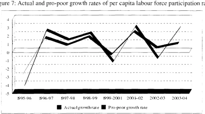
In addition. Figure 7 makes an interesting point. What emerges from the figure is that the

pro-poor growth rate for labour force participation is more volatile than the actual or

market growth rate for the same variable. This suggests that labour force participation

among the poor is affected more by the business cycle of the economy. When the

economy is in recession, the labour force participation rate for the poor tends to fall

sharply more than the national average. When the economy is in recovery. the labour

force participation for the poor tends to rise much faster than the national average.

Tab1e 5: Growth rates of per capita labour force par1icipation rate

Period Actual growth rate Pro-poor growth rate Gain( + )floss( -) 01' growth

1995-96 -2.66 -4.28 -1.62

1996-97 1.75 2.39 0.63

1997 -98 0.86 1.22 0.35

1998-99 1.83 2.03 0.20

1999-2001 -0.33 -1.50 -1.17

200 1-2002 2.48 2.82 0.34

2002-2003 0.53 -1.02 -1.55

2003-2004 1.06 2.69 1.63

1995-2004 0.73 0.41 -0.32

1995-2001 0.48 0.19 -0.29

2001-2004 1.27 1.24 -0.03

Source: authors' calculation based on Pl\'AD

Figure 7: Actual and pro-poor growth rates of per capita labour force participation rate

-'

U ｾＭＭＭＭｾｉＭＭＭＭＭＭＭＭＭＭＭＭＭＭＭＭＭＭＭＭﾭ

-1

-3

J- _________________________________________________________ _

-5

t... _ _ _ _ _ _ _ _ _ _ _

..

B95-96 B96-97 B97 -98 P98-99 P99-2OO I 200 ｾＰＲ＠ 2002-03 2003-04

• Actualgn:1\\thrate • Pm-poor gro\\th r,He

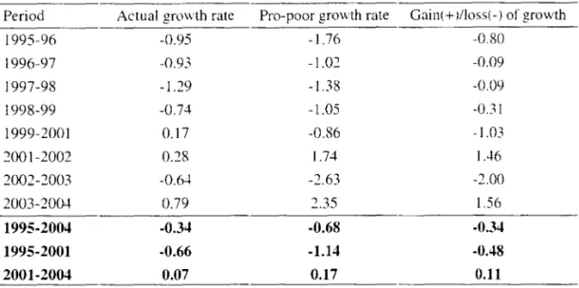
VIII.2 Employment

The employment rate is defined as the ratio of per capita employment to per capita labour

force participation rate.12 As indicated by Table 6. overall employment growth has been

negative over 1995-2004. The job growth rate of -0.66 percent per annum in the first

period has become positive in the second period, at 0.07 percent per annum. This

suggests that overall job growth in the labour market has been rather sluggish for the

period. 1995-2004. As far as employment growth for the poor is concemed, it has been

pessimistic in the entire period. anti-poor in general. However. employment among the

poor has become pro-poor in the second period. As shown in Figure 8. employment

growth was strongly in favour of the poor in 2001-02 and also in 2003-04 but highly

against the poor in 2002-03.

12 l\'ote that this is the usual definition of the employment rate: the percentage of labour force that is

Table 6: Growth rates of per capita employment rate

Period Actual growth rate Pro-poor growth rate Gain( + J/loss( -) 01' growth

1995-96 -0.95 -1.76 -0.80

1996-97 -0.93 -1.02 -0.09

1997-98 -1.29 -1.38 -0.09

1998-99 -0.74 -l.05 -0.31

1999-2001 0.17 -0.86 -1.0.3

2001-2002 0.28 1.74 IA6

2002-2003 -0.64 -2.63 -2.00

2003-2004 0.79 2.35 1.56

1995-2004 -0.34 -0.68 -0.34

1995-2001 -0.66 -1.14 -0.48

2001-2004 0.07 0.17 0.11

Source: authors' calculatioll based 011 PKAD

Figure 8: ActuaI and pro-poor growth rates of per capita employment rate

ＯｾＭＭＭＭＭＭＭＭＭＭＭＭＭＭＭＭＭＭＭＭＭＭＭＭＭＭＭＭＭＭＭＭＭＭＭＭＭＭＭＭＭＭＭＭＭＭＭＭＭＭＭＭＭＭＭＭ

3

2

1 _____________________________________ _

'I

11

_ _ _ _ _ _ _ _ ....J

-I i

-2 I -3

1995-96 1996-97 l'}97-9S 1998-99 1999-2001 2001--02 2002-03 2003-04

• !\ctualgmwhratc • Pro-poor gmv.th rate

VIII.3 Hours of work per employed person

The hours of work per employed person refers to the ratio of hours worked per person to

per capita employed persons in the household. Table 7 presents both actuaI and pro-poor

growth rates of hours of work per employed person. The results reveaI that while the

number of weekly hours per employed person has reduced over time. it has been

poor in general. These findings suggest that there has been a problem with

underemployment in the economy during the period 1995-2004. This underemployment

problem has become more serious in the second period (2001-2004) relative to the first

period (1995-2001). This has also happened to the poor. On lhe whole. while both

employment and labour force participation rales for the poor have improved in the period

2001-2004, the number of their working hours have declined in the same period.

Table 7: Growth rates of hours of work per employed person

Period Actual growth rale Pro-poor gnm·th rate Gain( + )/Ioss( -) of growth

1995-96 2.12 2.59 0,47

1996-97 -l.21 -1.75 -0.54

1997-98 -0.05 -0.07 -0.02

1998-99 -1.51 -2.35 -0.84

1999-2001 0.78 1.08 0.29

2001-2002 -1.56 -1.82 -0.26

2002-2003 -0.30 -1.50 -1.19

2003-2004 -0.43 0,44 0.87

1995-2004 -0.25 -0.41 -0.17

1995-2001 -(l.()7 -0.21 -0.14

2001-2004 -0.72 -1.01 -0.29

Source: authors' caIculation based on P!,;AD

Figure 9: Actual and pro-poor growth rates of hours of work per employed person

ＬｾＭＭＭＭＭＭＭＭＭＭＭＭＭＭＭＭＭＭＭＭＭＭＭＭＭＭＭＭＭＭＭＭＭＭＭＭＭＭＭＭＭＭＭＭＭＭＭＭＭＭ

ＭＭＭＭＭＭＭＭＭＭＭＭＭＭＭＭＭＭＭＭＭＭＭＭＭＭＭＭＭＭＭＭＭＭＭＭＭＭＭＭＭＭＭＭＭＭＭＭＭｾ＠

2

-I

2

-3

1995-96 1996-97 1997-98 199X-99 1999-2m] 2001--02 2oo2-D3 2lXB-D4

VIII.4 Productivity

In this study. per capita productivity is defined as per capita labour income per hour

worked. According to Table 8. per capita productivity has been declining over time.

Productivity deteriorated sharply in the second period in particular. However. per capita

producti vity has been pro-poor, improving from 0.18 percent per annum in the first

period to 0.56 percent per annum in the second period. The pro-poorness of productivity

has made a positive contribution to a reduction in inequality over the period. in particular

the second period. 2001-04. As Figure 10 illustrates. per capita productivity was highly

pro-poor in 2003-04.

Table 8: Growth rates of per capita productivity

Period Actual growth rate Pro-poor growth rate Gain( + )!Ioss( -) or growth

1995-96 2.65 -3.77 -6.41

1996-97 0.71 4.09 3.38

1997-98 -1.18 4.20 5.39

1998-99 -5.80 -2.01 3.79

1999-2001 -0.23 -2.26 -2.02

200 1-2002 -1.78 4.50 6.28

2002-2003 -6.74 -10.04 -3.31

2003-2004 1.86 10.76 8.90

1995-2004 -1.63 -0.05 1.58

1995-2001 -1.05 0.18 1.23

2001-2004 -2.67 0.56 3.23

Source: author,' caJculation based on PNAD

Figure 10: Actual and pro-poor growth rates of per capita productivity

.

ｌｾ＠

i U

-5

-lO

'! - - - - --- - -- - --- -- ---- -- -- - --- -- -- --- -- - -- - - - -.

-15

lY95-96 19%-97 1997-98 1998-99 1999-200 1 2001-02 2002-03 2003-04

• Actual growth rat. Pro-poor growth rate

People acquire human capital through schooling, It is general1y beIieved that an increase

in human capital improves people's earning potentiaI. As can be seen from Table 9, that

per capita schooling of working members within household had increased at an annual

rate of 2.34 percent in the first period. 1995-2001. In the subsequent period (2001-2004).

the growth rate in the years of schooling has been 4.04 percent per ami.um. Thus, in the

2000s there has been a dramatic improvement in education among working population in

BraziI. More importantly, the growth rate of social weIfare calcuIated from the years of

schooling has been 6.47 percent per annum during the same period. This suggests that

the expansion of education has been pro-poor. In other words. inequaIity in schooling has

been on the decline. This pro-poor expansion of education is generally expected to result

in a higher productivity in the economy. particularIy among the poor.

There exists no monotonic relationship between productivity and leveI of schooling. If an

expansion of schooling is accompanied by a reduction in returns from education. then

productivity in the economy may even falI. This is exactly happening in BraziI. It is

evident from Figure 11 that average returns from per year of schooling have been falling

monotonical1y since 1996. The fall in educational returns has offset the increase in the

average years of schooling. The fall in returns from schooling can be expIained in terms

Another factor that can impact productivity is changes in relative returns from education.

All households do not enjoy the same rates of returns for the same leveI of schooling.

Changes in relative retums over time have also effects on both growth rate in the mean

income and income inequality. The impact of changes in relative retums on growth and

inequality is measured in the next section.

Table 9: GrO\\!th rates of per capita years of schooling. \\!orking members

Period Actual growth rate Pro-poor growth rate Gain( + )/Ioss( -) of growth

1995-96 l.09 -1.30 -2 . .38

1996-97 2.03 2.52 0.49

1997-98 2.26 4.49 2.24

1998-99 2.5.3 4.68 2.15

1999-2001 2.96 2.03 -0.93

200l -2002 5.25 8.75 3.50

2002-2003 2.81 3.96 1.16

2003-2004 4.49 7.54 3.05

1995-2004 2.99 3.95 0.97

1995-2001 2.34 2.80 0.46

2001-2004 4.04 6.47 2.43

Source: authors' ca1culation based on PNAD

Figure 11: A verage Rate of Retums from per year of schooling. working members

15 ｲＭＭＭＭＭＭＭＭＭＭＭＭＭＭＭＭＭＭＭＭＭＭＭＭＭＭＭＭＭＭＭＭＭＭＭＭＭＭＭＭＭＭＭＭＭＭＭＭＭＭＭＭＭｾ＠

1-l - - - -I

C{j

,.. 12 -E

ｾ＠ 11

---0.9 L---_ _ _ _ _ _ _ _ _ _ _ _ _ _ _ _ _ _ _ _ _ _ _ _ _ - - - - _

li 95 fl97 li98 2001 2(X)2 2003

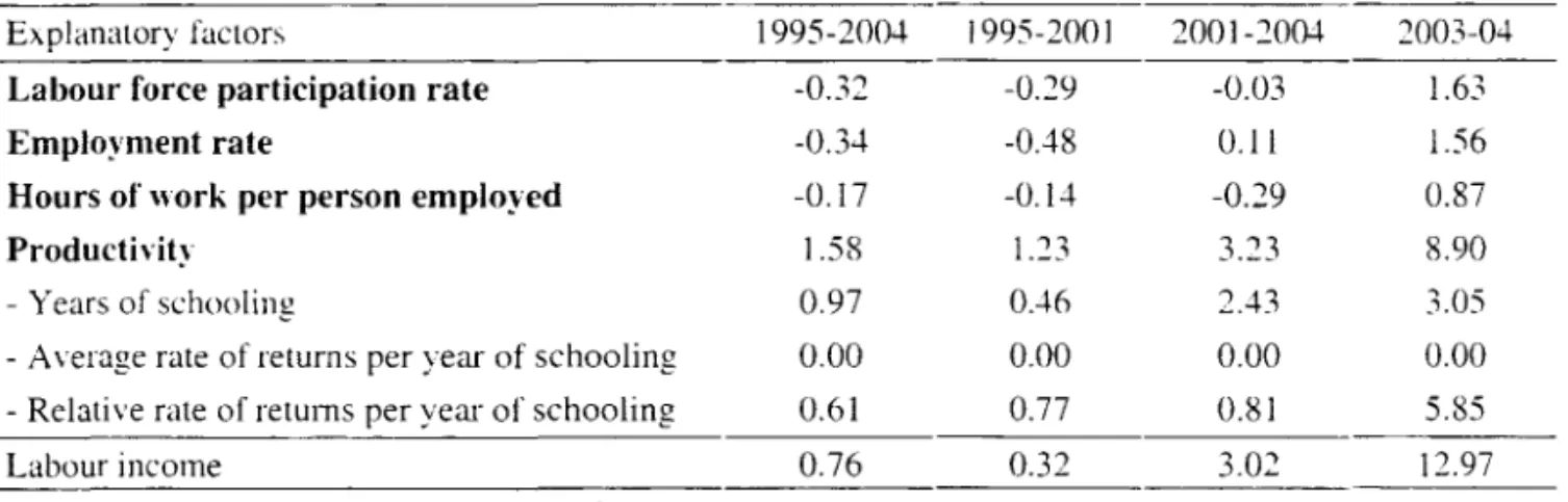
VIII. 6 Decomposition analysis

50 faL \ve have examined four factors in tum that have impacts on the pro-poor grmvth

rate of per capita labour income. These factors are now put together by means of lhe ne\\'

decomposition methodology we are proposing in this study. The decomposition reslllts

are presented in Tables 11-13.

Table 11: Explaining growth rates of per capita real income

Explanatory factors 1995-2004 1995-2001 ＲＰＰＱＭＲＰＰｾ＠ ＲＰＰＳＭＰｾ＠

Labour force participation rate 0.73 0.48 1.27 1.06

ｅｭｰｬｯｾＧｭ･ｮｴ＠ rate -0.34 -0.66 0.07 0.79

Hours of work per person employed -0.25 -0.07 -0.72 -0,43

Productivity -1.63 -1.05 -2.67 1.86

- Years af schooling 2.99 2.34 ｾＮＰＴ＠ ｾＬＴＹ＠

- A verage rate of retums per year 01' schaoling ＭｾＮＶＲ＠ -3.38 -6.71 -2.63 - Relative rale of retums per year of schooling -0.00 0.00 0.00 -O .e)O

Totallabour income -1,49 -1.30 -2.05 3.28

Source: authors' ca1culatiol1 based 011 PNAD

The per capita labour income declined at an annual rate of 1.49 percent in the entire

period from 1995 to 2004. The factors contribllting to this decline are employment rate.

hours of work and productivity. The employment rate and hours of work contribllted to a

decline in growth rate by 0.34 and 0.25 percent. respectively. The decline in prodllctivity

was the major factor that contributed to a decline of growth rate by 1.63 percent. Despite

the weak labour market. the labour force participation rate increased at an annual rate of

0.73 percent, which made a positive contribution to growth by the same magnitude.

It is also evident that the work force in Brazil is getting more educated. The years of

schooling of the labollr force increased at an annual rate of 2.99 percent during the

1995-04 period, which contributed to an increase in prodllctivity by the same rate (2.99

percent). The expansion of education has been accompanied by a decline in the average

rates of retum from schooling at an annual rate of 4.62 percent. This suggests that the

demand in the labour market has been sluggish and that growth in wage rates has 110t

A similar story emerges when we look at the sub periods: 1995-0 I and 2001-04.

However. the story changes when we look at the changes occuned during 2003-04, when

the per capita labour income increased by 3.28 percent. Again. productivity was the

major factor contributing to the growth. but in this case it contributed a positive rate of

1.86 percent. The labour force participation rate increased by 1.06 percent, while the

employment rate increased by 0.79 percent. This implies that per capita employment rate

(i.e. the sum of the labour force participation rate and the employment rate) increased by

1.85 pcrcent. From these observations. we can conclude that the labour market turned

around very strongly in the 2003-04 period. The rate of return from schooling declined at

much slower rate of only 2.63 percent despi te the fact that years of schooling of the work

force increased at a faster rate of 4.49 percent.

Table 12: Explaining pro-poor growth rate of money-metric social welfare

Explanator)' factor, 1995-2004 1995-2001 2001-2004 2003-04

Labour force participation rate OAI 0.19 1.24 2.69

Employment rate -0.68 -1.14 0.17 2.35

Hours of work per person employed -OAI -0.21 -1.01 OA4

Productivity -0.05 0.18 0.56 10.76

- Years of schooling 3.95 2.80 6A7 7.54

- A verage rate of returns per year 01' schooling -4.62 -3.38 -6.71 -2.63 - Relative rate of returns per year of schooling 0.61 0.77 0.81 5.85

TOlallabour income -0.73 -0.97 0.97 16.24

Source: authors' calculation based on PKAD

Table 12 presents the growth rates of money metric social welfare. The growth rate of

per capita social welfare is -0.97 percent in the first peliod (1995-01) but increases to

0.97 in the second period (2001-02). The factors that are contributing positively to

growth in the second period are labour force pat1icipation rate, employment rate and

productivity. The productivity growth rate of 0.56 percent is further decomposed into

three factors: (i) years of schooling, which contributes to an increase in the growth rate of

productivity by 6.47 percentage points: (ii) average rate of return which contributes to a

decline in productivity by 6.71 percentage points: and (iii) relative rate of returno which

contributes to an increase in the growth rate of productivity by 0.81 percentage points.

Different households enjoy different rates of rctum from per year of schooling. These

differences may be caused by a host of variables including age and gender of eamers in

household. number of eamers in household. sectors of employment by workers in

household. educationallevels of working members and so on. Thus. relative rates of

retums will also change due to a multitude of factors. The changes in relative rates of

return will not affect the growth rate of the mean labour income but they will affect the

social welfare. which is sensitive to changes in relative distribution. Our empilical results

show that the changes in relative rates of retum have contributed to the increase in the

growth rate of social welfare by 0.81 percentage points. This is a small contribution

compared to the decline in welfare that is caused by the average rate of retum from

schooling.

Table 13 presents gains (and losses) of growth rates due to pro-pOOl' (and anti-poor)

growth. The labour income has become highly pro-poor in the 2001-04 period

contributing to gains in the growth rate of 3.02 percent. In 2003-04. the gain in growth

rate increased to 1 2.97 percent. which indicates a large reduction in inequality. Thus. the

Brazilian labour market has become highly pro-poor in 2003-04. Productivity is the most

important factor contributing to gains in the growth rate of 8.9 percent. Schooling

conuibutes to gains in the growth rate of about 3 percent. The relative rates of retums

from schooling have beco me highly favourable to the poor contributing to gains in the

growth rate of 5.8 percent.

Table 13: Explaining gains and losses in growth rates

Explanatory factor, 1995-2004 1995-2001 2001-2004 2003-04

Labour force participation rate -0.32 -0.29 -0.03 1.63

Employment rate -0.34 -0.48 0.11 1.56

Hours of work per person employed -0.17 -0.14 -0.29 0.87

ｐｲｯ､ｵ｣ｴｩ｜Ｇｩｴｾ＠ 1.58 1.23 3.23 8.90

- Years of schooling 0.97 0.46 2.43 3.05

- A verage rate of returns per year of schooling 0.00 0.00 0.00 0.00 - Relative rate of retu1l1s per year 01' schooling 0.61 0.77 0.81 5.85

Labour income 0.76 0.32 3.02 12.97

Apart from productivity. the other labour market characteristics sllch as the labour force

participation rate. the employment rate and work hours per employed person have also

contribllted to a large reduction in inequality during 2001-04.

IX. Contribution of Income Sources to Growth

The separation of per capita total income into labour and non-labour components allO\vs

us to capture the main sources of the total growth patterns assumed. As we have

previously seen for the 1995-2004 period, total income average growth was -0.63 percent

while labour income grew at an average rate of -1.49 percent; ando non-Iabour income

grew at an average rate of 2.64 per annum. However. in order to see the contribution of

different income sources to total income - as we have done for the labour market

components - it is not sufficient to gauge the growth rates of different component ratios,

but also to take into aceount the relati ve weights of each income source in total income.

This point also applies to pro-poor growth and to the inequality aspects of social welfare.

The interaction between the high non-linearity ofthese last two concepts and the additive

nature of income sources create some difficulties. As a resulto a Shapely decomposition

was used to obtain each income source contribution to pro-poor growth. which is

explained in the Appendix. In general, the contribution of a given source to the total

growth of a particular social welfare concept is positively related to its initial weight and

to its relative rate of growth in the same period. In Table 14. we present the rates of

growth and the contributions to the rates of grO\vth of total income. together with its

labour and non-Iabour components.

In 1995. labour income amounted to 82.1 percent of total income. while the remaining

17.9 percent referred to non-Iabour. However. the main sources of growth, and in

particular pro-poor growth sources. relied on the latter. As shown in Table 14, the fall of

total income of -0.63 percent per year in the overall 1995-2004 period can be

decomposed into the adverse labour income contribution of -1.17 percent per year and the contribution of non-labour income of 0.54 percent per year.