TESE
apresentada como requisito para a obtenção do título de Doutor da Universidade Federal de Minas Gerais e da Université d’Avignon et des Pays de Vaucluse
(Cotutella)
Composition, phenology and restoration of campo rupestre
mountain grasslands - Brazil.
Composição, fenologia e restauração dos campos rupestres - Brasil.
Soizig Le Stradic
A tese foi defendida dia 14 de dezembro de 2012 perante a seguinte banca:
William J. Bond Professor
University of Cape Town, South Africa Relator Grégory Mahy Professor
Université de Liège Belgium Relator
Gerhard E. Overbeck Dr., Professor Adjunto
Universidade Federal do Rio Grande do Sul, Brazil Examinador Giselda Durigan Dr., Pesquisadora
Instituto Florestal do Estado de São Paulo, Brazil Examinador J.-P. de Lemos-Filho Professor
Universidade Federal de Minas Gerais, Brazil Examinador Elise Buisson Dr., Professor Adjunto, H.D.R.
Université d’Avignon et des Pays de Vaucluse, France Orientadora
Geraldo W. Fernandes Professor
Universidade Federal de Minas Gerais, Brazil Co-orientador
Essa tese foi preparada no Institut Méditerranéen de Biodiversité et d’Écologie e no Laboratório de Ecologia Evolutiva e Biodiversidade
Université d’Avignon et des Pays de Vaucluse
École doctorale 536 «Sciences et Agrosciences»
THESE
présentée pour l’obtention du grade de Docteur de l’Universidade Federal de Minas Gerais & de l’Université d’Avignon et des Pays de Vaucluse
(Cotutelle)
Composition, phenology and restoration of campo rupestre
mountain grasslands - Brazil.
Composition, phénologie et restauration de pelouses d’altitude, les
campos rupestres - Brésil.
Soizig Le Stradic
La thèse a été soutenue le 14 Décembre 2012 devant le jury composé de:
William J. Bond Professeur
University of Cape Town, South Africa Rapporteur Grégory Mahy Professeur
Université de Liège Belgium Rapporteur
Gerhard E. Overbeck Docteur, Maître de Conférences
Universidade Federal do Rio Grande do Sul, Brazil Examinateur Giselda Durigan Docteur et chargé de recherche
Instituto Florestal do Estado de São Paulo, Brazil Examinateur J.-P.de Lemos-Filho Professeur
Universidade Federal de Minas Gerais, Brazil Examinateur Elise Buisson Maître de Conférences, H.D.R.
Université d’Avignon et des Pays de Vaucluse, France Directrice
Geraldo W. Fernandes Professeur
Universidade Federal de Minas Gerais, Brazil Co-directeur
Thèse préparée au sein de l’Institut Méditerranéen de Biodiversité et d’Écologie et du Laboratório de Ecologia Evolutiva e Biodiversidade
École doctorale 536 «Sciences et Agrosciences»
Chego à sacada e vejo a minha serra, a serra de meu pai e meu avô,
de todos os Andrades que passaram e passarão, a serra que não passa.
Era coisa dos índios e a tomamos
para enfeitar e presidir a vida neste vale soturno onde a riqueza
maior é a sua vista a cotemplá-la.
De longe nos revela o perfil grave. A cada volta de caminho aponta uma forma de ser, em ferro, eterna,
e sopra eternidade na fluência.
Esta manhã acordo e não a encontro.
Britada em bilhões de lascas
deslizando em correia transportadora
entupindo 150 vagões
no trem-monstro de 5 locomotivas
- trem maior do mundo, tomem nota - foge minha serra, vai
deixando no meu corpo a paisagem mísero pó de ferro, e este não passa.
Remerciements
7 Août 2012: j’attends le bus de Belo Horizonte au bord de la route, c’était mon dernier jour de terrain dans la Serra do Cipó. Une fois n’est pas coutume, je me décide à prendre un peu
d’avance et je commence à faire la liste des personnes qui ont participé de près ou de loin à la
réalisation de cette thèse.
La veille de rendre ce manuscrit: pour ne pas déroger à la règle, je finis cette section de remerciements au dernier moment.
Je tiens tout d’abord à adresser un énorme merci à Elise qui m’a permis de traverser l’Atlantique pour la première fois il y a presque 5 ans, d’avoir eu confiance en moi pour réaliser cette thèse, d’avoir dépensé une énergie folle à la recherche de financements, pour les innombrables relectures de projets/CV/lettres de motivation, pour avoir su garder le moral et remonter le mien, pour son enthousiasme, pour m’avoir fait partager ses connaissances en écologie et en restauration, pour l’aide sur le terrain, pour l’encadrement même à distance, pour m’avoir hébergé quand je descendais à Avignon et claro pour m’avoir fait partager son goût pour le Brésil, les pães de queijos et la samba, muito obrigada mesmo;
Quero também agradecer a Geraldo (o Geraldinho!), que aceitou que eu fizesse meu doutorado no LEEB, que me apoiou e acreditou nesse projeto, me dando liberdade para a realização de minhas ideias, por sempre apresentar um novo ponto de vista (ou dar mil ideias para um novo projeto) e transmitir sua alegria e seu entusiasmo pela pesquisa. Muito obrigada Ge;
I am grateful to Pr. William J. Bond, from the University of Cape Town (South Africa), Pr. Grégory Mahy, from the Gembloux Agro-Bio Tech, Université de Liège (Belgium), Dr. Gerhard E. Overbeck from the Universidade Federal do Rio Grande do Sul (Brazil), Dr. Giselda Durigan from the Instituto Florestal do Estado de São Paulo (Brazil), Pr. Jose Pires de Lemos Filho from the Universidade Federal de Minas Gerais (Brazil) and Dr. José Eugênio Côrtes Figueira from the Universidade Federal de Minas Gerais (Brazil) who have accepted to review this work and evaluate the oral defense;
Financial support for this thesis was provided by the French Ministry of Foreign affair (EGIDE: bourse Lavoisier & Collège doctoral franco-brésilien), the CNPq, the CNRS and the CEMAGREF/IRSTEA, the University of Avignon (Programme Perdiguier), the Federal University of Minas Gerais & the US Fish & Wildlife Service, the SFE;
Quero agradecer aos membros da banca de qualificação na UFMG: José Eugênio Côrtes Figueira, Yumi Oki e Frederico Neves, que ajudaram com correções e sugestões a esse trabalho; agradeço também ao programa de Pos-graduação ECMVS e a todos os professores que me mostraram um jeito de ensinar diferente da França e que avaliaram esse trabalho durante os seminários de avaliação; agradeço também a Frederico e a Cristiane da Secretaria que sempre responderam às minhas perguntas diversas e variadas ;
Muito obrigada a Patricia Morellato por acolher a Swanni e a mim em Rio Claro, por ter nos ajudado a descobrir o que tinha por trás dessas tabelas de fenologia, além de todas as discussões a esse respeito.Obrigada também a todo o laboratório de fenologia pela alegria ambiente e Alessandra Fidelis para todos os conselhos; meus agradecimentos também a Alan, sua família e Rafael por nos acolher na casa dele durante nossa estadia em Rio Claro; sua companhia foi ótima;
Agradeço também aos botanistas que colocaram nome nas minhas plantas (même si Erioc. petit pompom c’était aussi sympa): Benoit Loeuille (Asteraceae), Pedro Lage Viana (Poaceae), Renato de Mello-Silva (Velloziaceae), Livia Echternacht (Eriocaulaceae), Nara de O. Mota Furtado (Xyridaceae) & Fernando A. O. Silveira (Melastomataceae); quero agradecer também ao professore Alexandre Salino e Bruno por se disponibilizarem para que eu pudesse usar o herbário da UFMG;
I am also grateful to Alice N Endamne, Kolo D Wamba and Viviane Ramos who revised and improved greatly the english of this thesis;
Meus agradecimentos especiais para a Jucelino e Elena pela ótima companhia durante esse tempo todo na Serra do Cipó (aprendi português assistindo ao Jornal Nacional na casa de vocês), pelas comidas deliciosas, pelas noites de cinema no meio de nada, pelos churrascos que tinham que fazer quando a energia acabava ; quero agradecer também a Wellington que tentou me ensinar a jogar truco mas já esqueci as regras, tentou também me ensinar gírias malucas, por sua ótima companhia (raramente conheci alguém que falasse tanto héhé), foram muitas risadas e tempos bons com você; além disso agradeço a todo mundo com quem convivi na Serra : Cláudio, Wemerson, Evaldo, Ronaldo, Toni, Genário (ou Genimar !); o que seria de mim sem incentivo pra ir ao campo, guardarei para sempre lembranças dos pães de queijo com lingüiça de Chapéu do sol ;
la fonction pyrolyse de votre four);
Obrigadão Daniel N., você foi o primeiro a me fazer descobrir os campos rupestres. Me lembro ainda do dia em que você me mostrou seus campos rupestres de “sonho” ! Obrigada por compartilhar seu amor por essas plantas, muito obrigada mesmo por sempre se entusiasmar com esse projeto e compartilhar tudo que você sabe, e por todas as releituras que você fez dessa tese. Um super obrigada também para Lêle (Pr. Fernando agora), pela ajuda no campo, pela ajuda com a germinação, com as releituras das partes dessa tese, por dar idéias ótimas, por ser muito e sempre entusiasmado e por sua alegria contagiante. Muito obrigada também à Vanessa por sua amizade, sua inestimável ajuda e sua disponibilidade para cuidar e contar tantas sementes! (inclusive durante Natal!).
Un grand merci également à Kevin, pour toutes les petites graines que tu as dû couper, les centaines de données de phénologie que tu m’a aidée à rentrer, les plats du chef préparé dans la Serra, les nombreux coups de bêches, toutes ces touffes qu’on a transplantées et les feuilles qu’on a comptées.... bon au final j’ai quand même réussi à te convaincre de ne pas faire de terrain pendant le doctorat, j’ai peut être abusé! Merci à Pauline pour le terrain, il y a eu beaucoup d’attaque de mouches mordeuses mais nous sommes restées fermes, et aussi pour les pauses petits gateaux et bière : je me sens moins coupable comme ça.
Um carinho muito especial para meus colegas do LEEB: a Renata que carregou pra mim muito solo pra lá e pra cá na Serra e que ficou firme no episódio da Jibóia, para a amizade, as baladas, o metrô às 6h da manhã em SP e as cervejas. A Cris e a Camila porque diversão é bom, mesmo se a gente demora 6 meses para se encontrar às vezes, o importante é continuar a se encontrar; o Marcelzinho, que me agüentou durante todo esse tempo que passamos juntos na salinha do fundo; mesmo se seus gostos musicais duvidosos me dão medo às vezes e mesmo sem camaro amarelo : você é doce!; meus colegas da famosa salinha do fundo que colocaram muita alegria nesses 4 anos: Miltinho que já virou Lord, Newtinho (vou ter que pegar dicas para conseguir ficar calma igual você!), Fernando, Manu, Tate e as famosas meninas do A2: Yumi (obrigada mesmo por sua disponibilidade imensa para sempre ajudar qualquer um dentro nós), Carol, Fabíola, Ana, Barbara, Leandra e me perdoem se me esquecer de um monte de gente, mas tem tanta gente!!
terrain pendant les vacances), Anlor, Max, Clem, Eric, Noum, Tristan, Antho,
Nico, Marie, pour leur amitié (il y a 25 ans nous étions déjà ensemble dans les bacs à
sable), parce que d’avoir toujours eu un comité d’accueil à la descente de l’avion ça n’a pas de prix surtout quand il est question de victuailles tels que du pâté, du saucisson, du vin et des projections de sylvain Mirouf, pour aider à porter les valises jusqu’au RER dans l’autre sens, et aussi pour les messages de soutien quand y’a eu besoin ; un énorme merci également à Estelle, Maria et Aurélie pour leur amitié, leur soutien, les messages d’encouragement ; un grand merci également à Tony qui m’a apportée tout son soutien et m’a encouragée quand j’ai fait mes premiers pas au Brésil.
Enfin, et surtout, je remercie toute ma famille (Sébastien inclu bien sur !), mon parrain et ma marraine, pour leur soutien, les messages d’encouragement, les Noëls au mois d’Août, pour le ravitaillement en mets gastronomiques divers et variés qui ont mis un peu de Bretagne sous mes tropiques (sauté de veau, palets bretons, paté henaff, foie gras, rillettes, St Emilion, Gewurztraminer); plus particulièrement mes parents, Gaëlle et Renan qui m’ont toujours soutenue et encouragée, et ont accepté mon absence, pour les nombreux dimanches aprés-midi sur skype, pour être devenue ce que je suis aujourd’hui; partir n’est jamais une chose facile mais nécessaire pour gouter au plaisir de revenir.
Merci aussi à Daniel T., pelo apoio e pela compreensão, pela música (inclusive Roberto Carlos domingo de manhã), pela poesia (que seja Hölderlin ou Anderson Silva), pelas viagens, por agüentar de mim (sic) inclusive na fase final da redação, por aceitar que eu coloque bagunça na vida dele, para a confitura, as courbaturas e as dezenas de palavras que so existem entre a gente, por ser meu guichet de reclamações preferido, por ser o ombro onde podia chorar quando a saudade apertava, por corrigir meus textos em português à 1h da manhã, por fazer buracos na serra do Cipó até acabar com nossas mãos, por mais que tudo.
Merci à la Serra do Cipó, pour tous les bons moments que j’y ai passés, j’avais 22 ans quand j’ai débarqué là-haut, et, d’une certaine façon cet endroit m’a vu grandir. Une bonne BO est toujours utile, alors merci aussi à Radiohead, M.I.A, Seu Jorge, Chico Science et tant d’autres, écoutés en boucle et qui m’ont accompagnée quand il fallait grimper la montagne à 6h du matin. Hommage également à mes 3 pantalons de terrain dont il a fallu se séparer, mes dizaines de tee-shirts usés par le soleil, la douzaine de crayons et de gommes perdue dans les campos, mes chaussures de terrain mortes pour la recherche et la caravane qui est partie en cendre.
Index
Acknowledgements, Agradecimentos & Remerciements ... ix
Index ... xiv
List of Tables ... xviii
List of figures ... xxii
Introduction ... 1
1. Context ... 1
2. Objectives ... 4
3. Restoration ecology ... 7
3.1. Definitions ...7
3.2. Goals & Reference Ecosystem ...8
3.3. Type of intervention ...9
3.4. Legislation ... 10
3.5. Restoration Ecology & Community Ecology ... 10
4. Community Theory ... 11
4.1. Ecological community ... 11
4.2. Community ecology ... 12
4.3. Disturbance & Resilience ... 13
4.4. Succession: How do ecosystems change following a disturbance? ... 15
4.5. Assembly rules: How do species assemble into communities? ... 16
5. Biological model ... 18
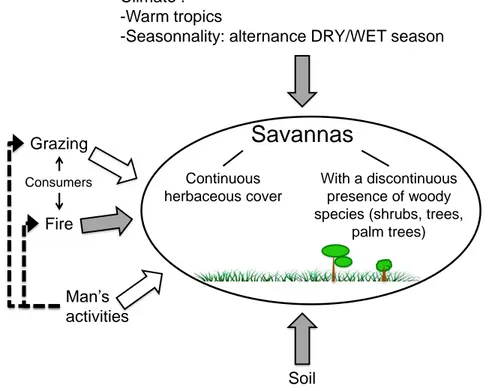
5.1. Savanna ecosystems ... 18
5.1.1. Definition ... 18
5.1.2. Geographic distribution ... 19
5.1.3. Main processes controlling savannas... 20
5.2. Cerrado ... 22
5.2.1. What is the Cerrado? ... 22
5.2.2. The controversial Cerrado ... 23
5.2.3. Brief history of the evolution of the Cerrado ... 25
5.3. Campos rupestres ... 26
5.3.1. Definition ... 26
5.3.2. Espinhaço range ... 26
5.3.3. Characteristics of the campos rupestres ... 28
5.3.4. What about the terminology? ... 31
5.3.5. Are campos rupestres included in the Cerrado? ... 32
5.4. Current Threats on Mountains ecosystems: focus on the campos rupestres .. 33
6. Study areas: Serra do Cipó campos rupestres ... 34
6.1. Geographic situation ... 34
6.2. Climate ... 35
6.3. Study sites ... 35
Chapter 1 - Baseline data for the conservation of campos rupestres: Vegetation
heterogeneity and diversity. ... 41
1. Introduction ... 43
2. Material and Methods ... 46
2.1. Study area and sites ... 46
2.2. Soil analyses ... 46
2.3. Plant survey ... 47
2.4. Statistical analyses ... 48
3. Results ... 50
3.1. Soil analyses ... 50
4.2. Similarities between the two grassland types ... 60
4.3. Differences between the two grassland types... 61
5. Conclusions ... 63
Transition to Chapter 2 ... 65
Chapter 2 - Reproductive phenological patterns of two Neotropical mountain
grasslands... 67
1. Introduction ... 69
2. Material & Methods ... 71
2.1. Study area... 71
2.2. Plant survey ... 72
2.3. Statistical analyses ... 73
3. Results... 74
3.1. Flowering, fruiting and dissemination patterns in sandy and stony grasslands. . ... 75
3.2. Flower and fruit production among grassland types and among families ... 80
3.1. Phenology and fruit production of species co-occurring in both grassland types. ... 81
4. Discussion ... 83
4.1. Flowering, fruiting and dissemination patterns in sandy and stony grasslands. . ... 84
4.2. Flower and fruit production in sandy and stony grasslands. ... 87
4.3. Comparison between sandy and stony grasslands. ... 87
5. Conclusion ... 87
Transition to Chapter 3 ... 89
Chapter 3 - Degradation of campos rupestres by quarrying: impact, resilience &
restoration using hay transfer... 93
1. Introduction ... 95
2. Material and Methods ... 98
2.1. Study area... 98
2.2. Resilience of the campos rupestres ... 99
2.2.1. Vegetation ... 99
2.2.2. Soils ... 99
2.2.3. Seed banks ... 100
2.3. Restoration using hay transfer ... 100
2.4. Statistical analysis ... 103
2.4.1. Resilience ... 103
2.4.2. Restoration using hay transfer ... 104
3. Results... 105
3.1. Resilience of the campos rupestres ... 105
3.2. Vegetation establishment limitation ... 106
3.2.1. Site limitation ... 106
3.2.2. Few viable seeds in the soils ... 108
3.3. Restoration using campo rupestre hay transfer ... 110
3.3.1. Vegetation cover ... 110
3.3.2. Effect of substrate on the number of seedlings ... 111
3.3.3. Effect of the type of hay on the number of seedlings ... 112
3.3.4. Limitation ... 114
4. Discussion ... 114
4.1. Resilience of campos rupestres ... 114
4.2. Restoration using campo rupestre hay transfer ... 117
forb species of campos rupestres. ... 121
1. Introduction ... 123
2. Material and methods ... 125
2.1. Seed collection ... 125
2.2. Germination experiments ... 127
2.3. Pre-fire vs. post-fire germination ... 128
2.4. Evolutionary ecology of seed dormancy ... 129
2.5. Statistical analyses ... 129
3. Results... 131
3.1. Intraspecific patterns of seed germination requirements ... 131
3.2. Effects of fire-related cues ... 135
3.3. Viability ... 135
3.4. Pre-fire vs. post-fire germination ... 135
3.5. Evolutionary ecology of seed dormancy ... 138
4. Discussion ... 140
5. Conclusion ... 146
Transition to Chapter 5 ... 148
Chapter 5 - Restoration of campos rupestres: species and turf translocation as
techniques for restoring highly degraded areas. ... 150
1. Introduction ... 152
2. Material and Methods ... 155
2.1. Study area... 155
2.2. Species translocation ... 155
2.3. Turf transfer... 157
2.4. Statistical analysis ... 158
2.4.1. Species translocation... 158
2.4.2. Turf translocation ... 158
3. Results... 159
3.1. Species translocation ... 159
3.1.1. Effect of substrate type (natural VS. degraded substrate) and nutrient supply ... 159
3.1.2. Effect of the translocation period ... 161
3.1.3. At the species level: cases of Paspalum erianthum and Tatianyx arnacites... 162
3.2. Turf transplantation ... 162
3.2.1. Effects of the turf size ... 163
3.2.2. Effects of the turf origin ... 164
3.2.3. Effects of the substrate of the degraded area. ... 166
3.2.4. Reference grassland regeneration ... 167
4. Discussion ... 168
5. Conclusion ... 171
General Discussion ... 173
1. What do we want to restore? ... 173
1.1. Composition and structure of herbaceous communities of campos rupestres .... ... 173
1.2. From the regional species pool to the external species pool: patterns of reproduction in campos rupestres ... 175
2. Plant community dynamics after disturbance ... 176
2.1. Regeneration after a natural disturbance ... 176
2.2. Campos rupestres are not resilient to a strong disturbance ... 176
2.3. Drivers of plant community recovery ... 177
2.3.1. Dispersal filter ... 178
4. From restoration ecology to community ecology ... 185
Main considerations of this thesis ... 188
Perspectives ... 189
1. To increase studies at large scale and use functional traits ... 189
2. Effect of fire on reproductive phenology ... 190
3. Understanding regeneration after natural disturbance ... 190
4. Germination ... 192
5. Looking for new restoration techniques ... 192
Conclusion ... 193
References... 194
Appendix Chapter 1 ... 227
Appendix Chapter 2 ... 240
Appendix Chapter 3 ... 252
1. Introduction ... 252
2. Material and methods ... 253
2.1. Study site ... 253
2.2. Seed bank analysis ... 254
2.3. Statistical analysis ... 254
3. Results... 254
4. Discussion ... 256
5. References ... 258
Appendix Chapter 4 ... 261
RESUME ... 263
RESUMO ... 264
List of Tables
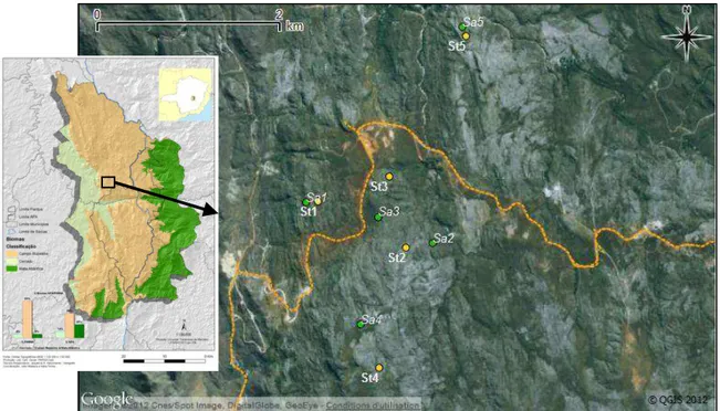
Table 1: Geographic coordinates of the 10 reference sites of campos rupestres. Florictic and phenological survey were realized on the 10 sites (Chapter 1 & 2); Sa1, Sa2, Sa3, St1, St2 & St3 were used as the references in the Chapter 3. ... 35
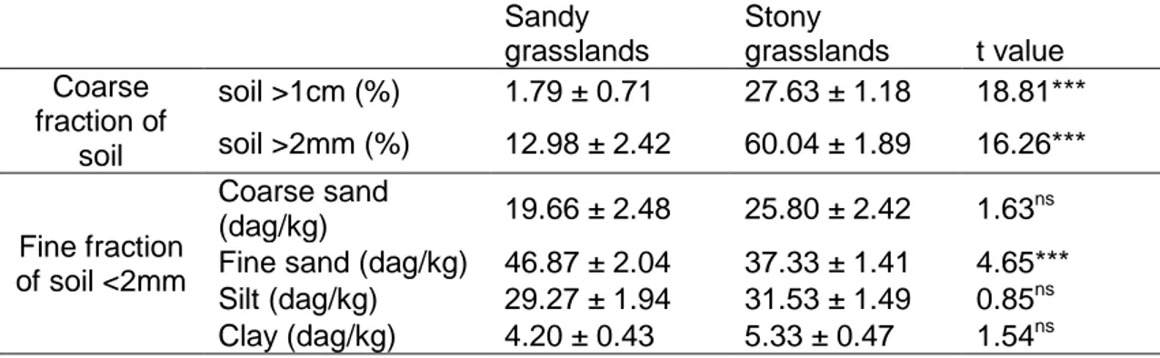
Table 2: Mean and standard error values of granulometric soil parameters, from soils collected in 5 sandy and 5 stony grasslands (3 samples / site , n=30). T-tests were run using separate variance estimates for the coarse fraction. ns: non-significant difference, *** :significant difference with P<0.001. ... 51
Table 3: Results of the two-way ANOVAs performed for chemical soil parameters, from soils collected in 5 sandy and 5 stony grasslands (3 samples / site / season, n=60. ns: non-significant difference, *: significant difference with P<0.05, ***: significant difference with P<0.001. ... 51
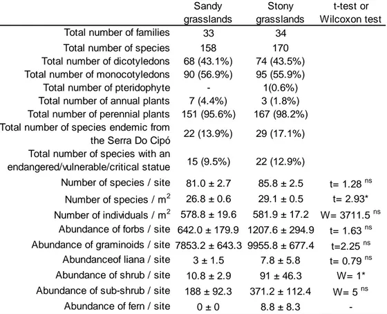
Table 4: Family and species distribution between sandy (5 sites, 15 quadrats / site, n=75) and stony grasslands (5 sites, 20 quadrats / site, n=100). ns: non significant difference, *:significant difference with P<0.05. ... 56
Table 5: Total number of species surveyed in both grassland-types, with number and percentage of perennial and annual species in each one and number and percentage of species participating in the reproductive phenology (flower, fruit and/or dissemination). ... 75
Table 6: Flowering, fruiting and dissemination data of sandy (Sa) and stony (St) plant communities at Serra do Cipó. Circular statistics (µ: mean vector, and r: parameter of concentration, Rao's spacing test: test of unimodality and Rayleigh tests). ... 76
Table 7 : Number and percentage of species according to the timing of flowering, fruiting and dissemination in sandy (Sa) and stony (St) grasslands. Pearson χ2 tests were performed, data marked with « ◊ » were not used in tests, species with continuous and sub-annual frequency patterns were not taken into account for the tests. ... 78
Table 8: Number of species and percentage according to the timing of flowering and phenological frequency in sandy (Sa) and stony (St (grasslands). A: annual frequency and SP: supra-annual frequency. Only A and SP species participating in the flowering phenophase were taken into account. ... 79
Table 9 : Number and percentage of species with long or short flowering (Fl.), fruiting (Fr.) and dissemination (Diss.) duration in sandy (Sa) and stony (St) grasslands. Long cycle is considered with a phenophase duration > 2 months and short cycle with a phenophase duration < or = 2 months. Species with continuous and sub-annual frequency patterns were not taken into account. w indicated that the χ2 tests
were realized without the data from transition season Dry/Rainy due to the low number of species. *: p-value<0.05 and **: p-value<0.01, ***:p-value <0.001. ... 80
Table 11: Average fruit production by site and number of fruits per individual for the 31 selected species. z indicates the result of GLM procedures with a quasibinomial error distribution and logit link function. * indicates significant differences with p<0.05. T-tests were performed using numbers of fruits per individual as dependent variables and grassland-types as categorical predictors, * indicates p<0.05. ... 83
Table 12: Dissimilarity matrix (Bray-curtis indices) of the plant composition between the degraded areas: with Latosol substrate (DL), stony substrate (DSt) and sandy substrate (DSa) and the reference grasslands: the sandy (Sa) and the stony (St) grasslands, based on species percent cover data (n=3 sites x 5 types of areas). . 105
Table 13: Mean and standard error values of soil texture, from soils collected in reference grasslands: 3 sandy, and 3 stony grasslands, and in degraded areas: 3 latosol, 3 sandy and 3 stony (3 samples x 3 sites x 5 types of areas, n=45). Kruskal-Wallis test were run for the coarse fraction and one-way nested ANOVA for the fine fraction. NS: non-significant difference, *significant difference with P<0.05, *** significant difference with P<0.001. ... 107
Table 14: Result of the one-way nested ANOVAs run on chemical soil parameters, from soils collected in reference grasslands: 3 sandy, and 3 stony grasslands, and in degraded areas: 3 latosol, 3 sandy and 3 stony (3 samples x 3 sites x 5 types of areas: n=45). NS: non-significant difference, * significant difference with P<0.05, *** significant difference with P<0.001. See Figure 4 for values. ... 107
Table 15: Number of germinated seeds and number of species found in the seed banks of the reference grasslands (sandy (Sa) and stony (St) grasslands) and of the three types of degraded areas (with latosol substrate (DL), stony substrate (DSt) and sandy substrate (DSa)) (n= 5 samples x 3 sites x 5 types of areas). Letters indicate significant differences according to the result of the GLM procedures (family: Poisson, link: log). ... 109
Table 16:: Dissimilarity matrix (Jaccard indices) of the seed bank composition between the degraded areas with latosol substrate (DL), stony substrate (DSt) and sandy substrate (DSa) and reference grasslands: the sandy (Sa) and the stony (St) grasslands based on presence-absence data (n=3 sites x 5 types of areas). ... 109
performed for Aristida torta, Lessingianthus linearifolius, Vellozia caruncularis,
Vellozia epidendroides, Vellozia resinosa, Vellozia variabilis, Xyris obtusiuscula and Xyris pilosa. ... 132
Table 19: Mean germination time MGT in days (mean with standard error) for each species according to each treatment. GLM procedures (with Gamma distribution) were performed for Aristida torta, Lessingianthus linearifolius, Vellozia caruncularis,
Vellozia epidendroides, Vellozia resinosa, Vellozia variabilis, Xyris obtusiuscula and Xyris pilosa. ... 133
Table 20: Germination synchrony (mean and standard error). Low values indicate more synchronized germination and high values indicate asynchronous germination. .. 134
Table 21: Viable, empty and dormant seeds (mean percentage and standard error) for each species. Dormant seeds were calculated as the final germination percentage over the total number of viable seeds. ND: non-dormant seeds. ... 138
Table 22: Number of individuals translocated in March 2011 (T0) and still surviving 3 months later in June 2011 (T3) with percent survival. Individuals were translocated to a degraded sandy area (DSa) and to a reference sandy grassland (RSa), broken into two groups, one with and added nutrient supply (N) and one without (n). To test the effect of nutrient supply and substrate type, GLM procedures were run with a binomial family distribution and logit link function. ns: non significant. ... 160
Table 23: Number and percentage survival of translocated individuals in December 2011 (T9) and in March 2011 (T12). Individuals were translocated to a degraded sandy area (DSa), and to a reference sandy grassland (RSa) broken into two groups, one with an added nutrient supply (N) and one without (n). To test the effect of nutrient supply and substrate type, GLM procedures were run on data recorded in March 2012, with a binomial family distribution and logit link function. ns: non significant. ... 161
Table 24: Number and percentage of surviving translocated individuals 3 months after the translocation, in June 2011 for individuals translocated in March 2011 and in February 2012 for individuals translocated November 2011. Individuals were translocated to a degraded sandy area (DSa) and to a reference sandy grassland (RSa) without added nutrients. 10 individuals for each species were translocated to DSa in March 2011, and for the other treatments, 5 individuals per species were translocated. To test the effect of the period of transplantation and substrate type GLM procedures were run with a binomial family distribution and logit link function. ns: non significant. ... 162
Table 25: Average number of individuals in 20x20cm and 40x40cm turfs translocated to degraded sandy substrate at T0 and T14 according to plant form: graminoids, forbs and sub-shrubs. Results of the LMER procedures are shown. ... 164
Eriocaulaceae species. There was no difference in sub-shrub number between TSa and TSt at T0, and their number increased with time in both kinds of turfs (Table 26).Table 26: Average number of individuals in 20x20cm turfs from sandy grasslands (TSa) and stony grasslands (TSt), translocated on degraded stony substrate at T0 and T14 according to plant form: graminoids, forbs and sub-shrubs. Results of the LMER procedures are shown. ... 165
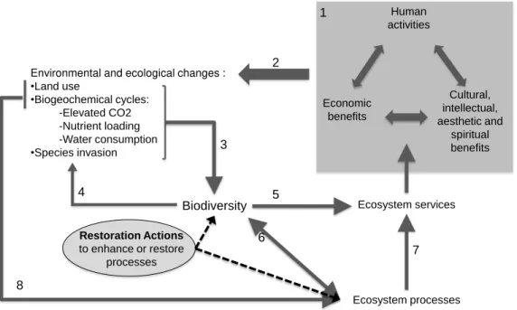
Figure 1: The role of biodiversity and restoration activities in global change. Human activities (1) are now causing environmental and ecological changes of global significance (2). Through a variety of mechanisms, these global changes contribute to changing biodiversity (3), and changing biodiversity feeds back on susceptibility to species invasions (4). Changes in biodiversity, can have direct consequences for ecosystem services impacting human economic and social activities (5). In addition, changes in biodiversity can influence ecosystem processes and feedback to further alter biodiversity (6). Altered ecosystem processes can thereby influence the ecosystem services that benefit humanity (7). Global changes may also directly affect ecosystem processes (8). Restoration actions are represented by dashed lines. (Adapted from Chapin et al. 2000, Palmer & Filoso 2012, Le Stradic unpublished)... 2
Figure 2: General overview of the organization of this thesis highlighting the steps recommended by the SER primer (SER 2004). Pale grey boxes correspond to the different steps developed in the thesis’s chapters, dark grey boxes represent the filters structuring the community (see section 4.5 Assembly rules: How do species assemble into communities?). Full black arrows: studies related to the reference ecosystem; full grey arrow: disturbance which destroyed pristine campos rupestres; dashed black arrows: we have assessed if degraded campos rupestres are resilient to strong disturbance from the external or internal species pool; dashed grey arrows: restoration techniques we have tested, act on different filters. ... 4
Figure 3: Schematic representation of the trajectory of a natural or semi-natural ecosystem over time. Full lines correspond to trajectories resulting from restoration interventions (reference ecosystem trajectory, rehabilitation or failure); dashed lines represent natural processes, or trajectories observed without interventions, and grey lines, the functions evolving in a third dimension, ASS (Alternative stable state). (Modified from Hobbs & Norton 1996, Prach & Hobbs 2008, Buisson 2011). ... 8
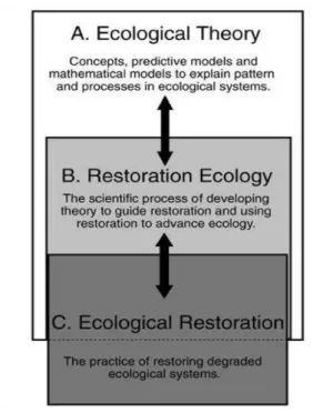
Figure 4: The relationship between ecological theory, restoration ecology, and ecological restoration can be viewed in a hierarchical fashion (Palmer et al. 2006)... 11
Figure 5: The theory of community ecology (from Vellend 2010) ... 13
Figure 6: The main processes / filters that structure a plant community. Each process/filter is represented by a pair of horizontal lines. Solid arrows depict the movement of species through the filters. Grey boxes indicate how ecosystem degradation may affect the different levels (inspired by Lortie et al. 2004, Fattorini & Halle 2004, Belyea 2004, Buisson 2011, Le Stradic unpublished). ... 17
Figure 7: Map of the tropical savannas according Bourlière 1983 ... 20
refer to Brazilian states: B=Bahia; DF=Federal District; GO=Goias; MA= Maranhão; MG=Minas Gerais; MS=Mato Grosso do Sul; MT=Mato Grosso; PA=Pará; PI=Piaui; RO=Rondônia; SP= SãoPaulo; TO=Tocantins. From Furley (1999). ... 22
Figure 10: Simplified structural gradient of Cerrado ecosystems (modified from Coutinho 1978) and representation of the ideology developed by some authors on the concept of Cerrado (Le Stradic unpublished)... 24
Figure 11: Campos rupestres considered as a physiognomy of the Cerrado (Le Stradic unpublished) ... 28
Figure 12: Map of the Espinhaço range showing the protected areas (Unidade de Concervação de Proteção integral). Number 1 is the Serra do Cipó National park where this study was realized Map from Biodiversitas fundation. ... 30
Figure 13: Map of the 10 study sites on the two main grassland-types of campos
rupestres: sites with the sandy substrate located on flatted areas (Sa) and sites with
stony substrate on slopes (St). The dashed line represents the highway MG-010. The inset shows a map of the environmental Protected Area (Area de Proteção Ambiental in Portuguese) Morro da Pedreira, which includes the Serra do Cipó National Park. (Map realized using Plano de manejo do PARNA Serra do Cipó
(2009), Google Earth image and QGIS). ... 36
Figure 14: Photographs of the campos rupestres from the Serra do Cipó, the general view a) during the dry season, b) during the wet season, c) sandy grasslands and d) stony grasslands. Photo credit S. Le Stradic ... 37
Figure 15: Map of the 9 degraded sites on three kinds of substrate: sites located on degraded latosol substrate (DL), on degraded sandy substrate (DSa) and on degraded stony substrate (DSt). The dashed line represents the highway MG-010. The inset shows a map of the environmental Protected Area (Area de Proteção Ambiental in Portuguese) Morro da Pedreira, including the Serra do Cipó National Park. (Map realized using Plano de manejo do PARNA Serra do Cipó (2009),
Google Earth image and QGIS)... 38
Figure 16: Degraded areas with a) degraded latosol substrate, b) degraded sandy substrate, c) degraded stony substrate. Photo credit S. Le Stradic. ... 39
Figure 17: Mean and standard error values of chemical soil parameters, from soils collected in sandy and stony grasslands (3 samples / 5+5 sites / 2 seasons, n=60). Open circles represent dry season and full circles rainy season. See Table 2 for two-way ANOVA results. ... 52
Figure 18: Ward clustering of a matrix of chord distances among sites (species data). . 54
Figure 19: Correspondence Analysis run on the matrix of plant percent cover in 1m² quadrats in the 5 sandy (Sa) and 5 stony (St) grasslands [175 points x 222 species]. Projection of the two first axes, axis 1 (29%) and axis 2 (18%). Inertia= 0.19,
Figure 21: Percentage of species according to plant forms. Sandy grasslands (black columns) and stony grasslands (grey columns) χ2=27.3, P<0.001 in sandy
grasslands and χ2=27.0, P<0.001 in stony grasslands. Lower-case letters indicate
differences between forms within sandy grasslands and capital letters between forms within stony grasslands (Multiple comparisons made using the Bonferroni correction). ... 57
Figure 22: Percentage of species according to life forms. Life-form: CH = Chamaephytes, GE= Geophytes, HE= hemicryptophytes, HL= hemicryptophyte lianas, NA= Nano-phanerophytes, TH = therophytes. Sandy grasslands (black columns) and stony grasslands (grey columns). χ2=24.25, P<0.001 in sandy
grasslands and χ2=25.96, P <0.001 in stony grasslands. Lower-case letters indicate
differences between forms within sandy grasslands and capital letters between forms within stony grasslands (Multiple comparisons made with the Bonferroni correction), * indicates differences between groups (t-test with unequal variances). ... 58
Figure 23: Number of species from the most-represented families in sandy grasslands (black columns) and stony grasslands (grey columns). (5 sites of each physiognomy, 15 1 m2 quadrats in sandy grasslands and 20 1m2 in stony grasslands). ... 58
Figure 24: Co-inertia results: a) Representation of the sites, arrow heads indicating floristic data and arrow tails indicating environmental data, b) Representation of the environmental data: soil composition and granulometry [10 points x 18 variables], c) Representation of the floristic data [10 points x 222 species]. Projection of the top two axes of the co-inertia: axis 1: 79.4%, axis 2: 10.5%. RV test observations= 0.61, P<0.01 (Monte-Carlo permutations). ... 59
Figure 25: The theoretical objective of the second chapter is to describe the phenological patterns of two herbaceous communities; the applied objective of the second chapter is to identify the species which produce seeds and thus might potentially colonize degraded areas. ... 66
Figure 26: Distribution of mean monthly temperatures (T°C) at 6h00 (open square) and 13h00 (full square), and cumulative rainfall (mm) between November 2009 and October 2011. Temperature data provided by G.A. Sanchez-Azofeifa, Enviro-Net project, University of Alberta. Rainfall data obtained by INMET (2012). ... 72
Figure 27: Flowering pattern in sandy (a) and stony (b) grasslands, fruiting pattern in sandy (c) and stony (d) grasslands and dissemination pattern in sandy (e) and stony (f) grasslands. These patterns were defined according to the number of species in each phenophase (based on the peak). Each species occurs only once. Arrows represented µ and the black circle the significant threshold. ... 77
donor sites, h: control without hay, G: with geotextile, w: without geotextile. Each treatment was replicated four times at each site in blocks. ... 102
Figure 30: Correspondence analysis on the matrix of species percent cover in 40cmx40cm quadrats in January 2010, in references areas: 3 stony (St) and 3 sandy grasslands (Sa) and in degraded areas: 3 with latosol substrate (DL), 3 with sandy substrate (DSa) and 3 with stony substrate (DSt) [288 points x 178 species]. Projection of the two first axes, axis 1 (17.2%) and axis 2 (16.4%). Inertia=0.17, p<0.001, Monte-Carlo permutations. ... 106
Figure 31: Mean and standard error values of chemical soil parameters, from soils collected in 3 sandy grasslands (Sa) and 3 stony grasslands (St), 3 degraded areas with latosol substrate (DL), 3 degraded areas with stony substrate (DSt), 3 degraded areas with sandy substrate (DSa) (3 samples / site / season, n=90). Full circles rainy season. See Table 3 for one-way nested ANOVA results. ... 108
Figure 32: Mean vegetation percent cover per 40cmx40cm quadrat according 5 types of areas: degraded areas with latosol substrate (DL), with sandy substrate (DSa), with stony substrate (DSt), reference sandy grassland (Sa) and reference stony grassland (St), and 2-3 level of 2 treatments: with hay from sandy grassland (HSa) / with hay from stony grassland (HSt) / without hay (h), and with geotextile (clear grey) / without geotextile (dark grey). Letters according the result of one-way nested ANOVAs, followed by Tukey post-hoc tests. ... 110
Figure 33: Correspondence analysis run on the matrix of the species abundance in February 2012 in 40cmx40cm quadrat after hay transfer in reference grasslands: 2 stony (St) and 2 sandy grasslands (Sa) and in degraded areas: 3 with latosol substrate (DL), 3 with sandy substrate (DSa) and 3 with stony substrate (DSt) [232 points x 161 species]. Some quadrats received hay and some not and some had geotextile and some not. Projection of the two first axes, axis 1 (17.2%) and axis 2 (14.2%). Inertia=0.23, p<0.001, Monte-Carlo permutations. ... 111
Figure 34: Mean number of seedlings occurring per 40cm×40cm quadrat on reference sandy grasslands (Sa) and on the 3 types of degraded areas: with latosol substrate (DL), with sandy substrate (DSa) and with stony sustrate (DSt) and 2 levels of 2 treatments: with hay (HSa) / without hay (h) and with geotextile (in clear grey) / without geotextile (dark grey). Letters indicate significant differences according to the result of the LMER procedures (family: Poisson, link: log), *: indicate difference between with and without geotextile. ... 112
without fire. Letters indicate significant difference according (a) GLM procedure (quasibinomial error distribution and logit link function) with F=25.43, p<0.001, (b) GLM procedure (Gamma error distribution and inverse link function) with F=52.78, p<0.001, (c) simple ANOVAs, followed by post-hoc tests (Tukey's “Honest Significant Difference”) F=31.70, p<0.001). ... 137
Figure 37: Reconstructed phylogenetic tree of the fifteen species studied, species with dormant seeds are underlined. ... 139
Figure 38: The objective of the fifth chapter is to test whether species and turf translocation are efficient techniques to restore campos rupestres. Both techniques aimed to overcome the dispersal filter. Using species translocation we expected to overcome the critical phase of the establishment in the degraded areas and to improve environmental conditions bringing together soil and translocated plant. Using turf translocation, we aimed to bring to the degraded areas i) a pool of target species, ii) soil of the reference ecosystem and iii) possible associated microorganisms (Carvalho et al. 2012); overcoming therefore the environmental filter and a part of the biotic filter... 149
Figure 39: Experimental design of species translocation. Experiment 1A was carried out in March 2011 at the end of the rainy season, while Experiment 1B was carried out in November 2011 at the beginning of the rainy season. ... 156
Figure 40: Experimental design of turf translocation carried out in March 2011 at the end of the rainy season. Experiment 2A was carried out in degraded sandy substrate DSa, while Experiment 2B was carried out in degraded stony substrate DSt. ... 157
Figure 41: Average vegetation cover (%) (mean ± standard error) on 40x40cm TSa (black squares with dashed line), on 20x20cm TSa (black squares with solid line) translocated in DSa and on 20x20cm TSt (black triangles and dashed line) and TSa (open squares and solid line) translocated in DSt over time (in months). ... 163
Figure 42: a) Average number of individuals and b) plant species richness in 40x40cm (dashed lines) or 20x20cm (solid line) translocated turfs in DSa over time (in months). Means within size were significantly different in May 2012 (T 14) (P <0.001) in both number of individuals and species richness. ... 164
Figure 43: a) Average number of individuals and b) plant species richness in 20x20cm TSt (dashed lines) and TSa (solid line) translocated in DSt over time (in months). Means within origin of turfs were similar in May 2012 (T 14) (P >0.05) in both number of individuals and species richness. ... 165
Figure 44: a) Average number of individuals and b) plant species richness in 20x20cm TSa transplanted in DSa (full squares) and in DSt (open squares) over time (in months). Means within each substrate were significantly different in May 2012 (T 14) in number of individuals (P <0.001) but similar in species richness (p=0.6). ... 167
disturbance; 3) Dispersal limitation did not allow the seed bank re-composition; 4) Hay transfer, which allows overcoming the dispersal filter, was not efficient to initiate vegetation establishment on degraded areas; 5) Some species among them Poaceae & Cyperaceae failed to germinate, other germinated well like Xyridaceae or Velloziaceae but were not able to establish on degraded areas, due to unfavorable germination conditions or because hay did not contain these species; 6) Probable root damages impede species establishment, just one species Paspalum
erianthum was reintroduce on degraded areas; 7) turf translocation was the most
successful restoration method allowing to introduce native species on degraded areas, but it was also the technique which most impacted the reference grasslands. ... 187
Figure 46: a) Bulbostylis paradoxa flowering a few days after a fire, and b) on sandy grasslands, lot of species flowering after a fire. (Photos S. Le Stradic) ... 190
Introduction
1.Context
In recent decades, the relationship between human society and the environment have been highlighted and have resulted in increasing awareness of the importance of
ecosystems in maintaining and improving the collective well-being of humanity, particularly because the world is now changing rapidly. Current economic development
and its impact on the environment are unsustainable: degradation of remaining natural habitats is decreasing long-term human welfare in favor of short-term economic gain.
Obviously this kind of development does not deliver human benefits in the way that it should: it increases the vulnerability of some of human populations and creates large
disparities around the world while the level of poverty remains high (Balmford et al. 2002, MEA 2005, Carpenter et al. 2006). Humans have already greatly altered Earth’s surface, especially through land-use changes, which are responsible for about half of terrestrial ecosystem transformations (Daily 1995, Vitousek et al. 1997, Chapin et al. 2000, Klink & Moreira 2002, Sala et al. 2005, Steffen et al. 2007), leading to the current Anthropocene
epoch (Steffen et al. 2007, Zalasiewicz et al. 2010).
Ecosystem services are the human benefits provided directly or indirectly by ecosystem
functions (i.e., the properties or processes of ecosystems) (Costanza et al. 1997). These services, such as climate stabilisation, drinking water supply, flood alleviation, crop
pollination, and recreation opportunities, among others (Osborne & Kovacic 1993, FAO 1998, Chapin et al. 2000, Balmford et al. 2002, MEA 2005, Sala et al. 2005), depend to
some extent on biodiversity (Rands et al. 2010) (Figure 1). However, many recent human activities have led to biodiversity erosion (Rands et al. 2010, Barnosky et al.
2011), altering functional diversity and modifying ecosystem properties (Loreau et al. 2001) (Figure 1). The Millennium Ecosystem Assessment (MEA 2005) report indicates
that 12–16% of the world’s species will be lost over the period of 1970 to 2050 due to habitat loss alone (Sala et al. 2005) and that currently approximately 60% of the ecosystem services are being degraded (MEA 2005). Biodiversity responses to
environmental changes (land use and climate changes) are likely to be complex (Chazal
further environmental changes (Chapin et al. 2000, Figure 1). According the
stability-diversity hypothesis, biostability-diversity should promote resistance and resilience to disturbance (McNaughton 1977, Pimm 1984, Tilman & Downing 1994, Chapin et al. 2000, McCann
2000, Loreau et al. 2001). This implies that ecosystem stability depends on the ability of communities to harbor species or functional groups that can respond to disturbances in
myriad ways. In this sense, biodiversity provides a kind of “insurance” against environmental fluctuations (Chapin et al. 2000, McCann 2000, Loreau et al. 2001).
Human activities Economic benefits Cultural, intellectual, aesthetic and spiritual benefits Ecosystem services Ecosystem processes Environmental and ecological changes :
•Land use
•Biogeochemical cycles: -Elevated CO2 -Nutrient loading -Water consumption
•Species invasion
1 2 Biodiversity 3 4 5 6 7 8 Restoration Actions
to enhance or restore processes
Figure 1: The role of biodiversity and restoration activities in global change. Human activities (1) are now causing environmental and ecological changes of global significance (2). Through a variety of mechanisms, these global changes contribute to changing biodiversity (3), and changing biodiversity feeds back on susceptibility to species invasions (4). Changes in biodiversity, can have direct consequences for ecosystem services impacting human economic and social activities (5). In addition, changes in biodiversity can influence ecosystem processes and feedback to further alter biodiversity (6). Altered ecosystem processes can thereby influence the ecosystem services that benefit humanity (7). Global changes may also directly affect ecosystem processes (8). Restoration actions are represented by dashed lines. (Adapted from Chapin et al. 2000, Palmer & Filoso 2012, Le Stradic unpublished).
Effective conservation of biodiversity is fundamental to maintaining ecosystem
processes, but the traditional arguments in support of ecosystem conservation alone are insufficient (Turner & Daily 2008, Rands et al. 2010). Marked economic benefits
preserve nature (Balmford et al. 2002, Ring et al. 2010, Nahlik et al. 2012). However
conservation in certain locales can be limited because the areas in question are either too small, too few, or too degraded to preserve biological processes and diversity
(Anderson 1995; Hobbs & Norton 1996). In this context, ecological restoration can be a viable strategy for enhancing biodiversity and improving ecosystem services
(Hilderbrand et al. 2005, Rey-Benayas et al. 2009, Bullock et al. 2011, Schneiders et al. 2012), especially with the development of Payment for Ecosystem Services (PES)
schemes, which are designed to compensate actions that maintain, improve, and provide some ecosystem services (Turpie et al. 2008, Farley et al. 2010, Farley &
Contanza 2010). The Strategic Plan for Biodiversity specifies that at least 15% of degraded ecosystems must be restored by 2020 (CBD 2011). Roberts et al. (2009)
emphasize that “our planet’s future may depend on the maturation of the young discipline of ecological restoration”. However, focusing ecological restoration on ecosystem services should not come at the expense of biodiversity conservation, and
damage prevention should always be considered first because restoration possibilities cannot be an excuse for ongoing damage or destruction of ecosystems (Young 2000,
Hobbs 2007, Hobbs & Cramer 2008). Young (2000) highlights the important points that 1) restoration can improve conservation efforts but has to remain a secondary resort to
the preservation of habitats and 2) the use of ex-situ “restoration”, such as mitigation, will never produce an outcome resembling the perfect reversal of habitat and population
2.Objectives
This thesis contributes both to 1) an improved theoretical understanding of the
functioning of a type of neotropical mountain grasslands, the campos rupestres and their dynamics following strong disturbances and 2) novel insights into the implementation of
restoration techniques for such environments (Figure 2).
Like all research in restoration ecology and ecological restoration projects, this thesis
follows the three steps outlined in the SER primer (SER 2004) (Figure 2):
1) Identify the reference ecosystem & gather information on it (Chap 1, 2 & 4); 2) Identify the disturbance, its effects and assess resilience (Chap 3);
3) Identify which restoration methods can provide an efficient means of initiating the resilience of degraded areas (Chap 3, 4 & 5.
external SP (Chap. 2)
Dispersal filter Community Environmental filter Biotic filter
What do we want to restore?
I
Identify the
Reference Ecosystem
(Chap. 1, 2 & 4)
III
Identify efficient
restoration
techniques (Chap. 3 & 5)
II
Identify the
disturbance &
its effects (Chap. 3)
Germination (Chap. 4)
Is the system resilient? (Chap. 3) Road construction
?
internal SP (Chap. 3 seedbank)
Species pool
As indicated, the first objective of this thesis is to identify and describe the reference
ecosystem (Chapters 1, 2 & 4) (Figure 2) and to answer the question, what do we want to restore? A clear definition of the restoration target is essential to developing a basis
for monitoring progress and for assessing restoration success. Fulfilling this first objective comes down to demonstrating that campos rupestres are a mosaic of
grasslands with at least two distinct plant communities (i.e. sandy and stony grasslands), each having specific compositional, structural and phenological patterns. One of our
goals in performing the phenological study is to define the local species pool, which means assessing global flower and fruit production and determining what species can
potentially contribute to recolonisation via their seeds.
The second objective is to identify the main effects of a strong disturbance on soil and
seed bank composition and to assess the resilience of campos rupestres (Chapter 3) (Figure 2); in other words, are campos rupestres resilient to strong disturbances? Land-use changes provide an opportunity to study vegetation recovery and community
assembly (Prach & Walker 2011). According to theoretical models, three main filters, which, when applied to the global species pool determine the ultimate community
structure. These are the dispersal, environmental and biotic filters (Keddy 1992, Lortie et al. 2004) (Figure 2). In order to establish whether restoration is actually necessary, we
surveyed plant community characteristics, chemical and physical soil properties, and seed banks, in the areas that were first degraded eight years ago by the harsh but
common activity of road construction-related quarrying. Our objective was to determine how this type of degradation modifies soil properties, and whether or not the internal
species pool recomposed itself with target species following the degradation. The main questions addressed in the third part of this thesis are (Chapter 3, 4 & 5) (Figure 2): Can we restore campos rupestres? By using restoration experiments, we identified the
factors that limit resilience by acting first on the dispersal filter, then we aimed to
overcome the dispersal filter and the germination and to improve environmental
conditions, and finally we aimed to overcome the dispersal, the abiotic and part of the biotic filters. Our ultimate aim was to identify efficient techniques for restoring these
species-rich grasslands along with, hopefully, some services they once provided. Some
evidence has shown that restoration actions that focus on biodiversity are also effective
even where it is incorrect to assume that restoring biodiversity must inevitably enhance
ecosystem services, or vice versa (Bullock et al. 2011).
The ecosystem in the present study is the campos rupestres, or tropical mountain
grasslands located into the Cerrado domain, or Brazilian savanna. We chose to work with herbaceous species because the herbaceous stratum is the quintessence of these
grasslands and regulates fundamental processes, such as post-fire recovery, water balance, annual productivity or mineral cycling (Sarmiento 1984). Moreover, in recent
decades, herbaceous ecosystems, which represent more than 31% of world vegetation, have been drastically damaged and fragmented throughout the world (Green 1990,
Hoekstra et al. 2005, Gibson 2009). Biodiversity scenarios indicate that grassland ecosystems, and tropical ecosystems in general, are expected to be the most strongly
impacted by land-use changes in the future (Chapin et al. 2000, Sala et al. 2000, 2005); in this context, the Cerrado has already been classified as a priority area for conservation due to the anthropogenic pressures that it faces (Myers et al. 2000,
Mittermeier et al. 2004, Hoekstra et al. 2005). It is therefore important to preserve and restore diverse grasslands since it can aim at conserving both biodiversity and locally
important ecosystem services, and this is particularly true of mountain grasslands (CBD 2004, MEA 2005).
3.Restoration ecology
3.1.
Definitions
Ecological restoration is the practice of restoring ecosystems and restoration ecology
is the science upon which this practice is based (SER 2004). Restoration ecology is
intended to offer clear concepts, models, methodologies and tools for practitioners. As will be discussed later, restoration ecology also plays an important role in ecological
theory.
Ecological restoration is also the process of intentionally aiding in the recovery of an
ecosystem that has been degraded, damaged, or destroyed (SER 2004). Ecological
restoration sensu stricto, is an intentional activity that initiates or accelerates
ecosystem recovery in order to re-establish all of the attributes of the reference ecosystem: its biotic integrity in terms of species composition and community structure, its functional processes, its sustainability in terms of overall resilience and resistance to
disturbances, its productivity, and its services (SER 2004, Clewell et al. 2005) (Figure 3). This objective is theoretical and often unrealistic: it is very difficult to achieve complete
restoration of an ecosystem back to its original state (Lockwood and Pimm 1999, Palmer et al. 2006, Choi et al. 2008, Hobbs et al. 2011). Alternative, less ideal ecological
restoration activities can also be carried out, and these usually fall under the designation ecological restoration sensu lato (SER 2004). Examples include such activities as
rehabilitation or reclamation (SER 2004) (Figure 3). Rehabilitation, in which
pexisting ecosystems are also taken as models, places its emphasis on the
Complex ity or fu nctio n Time St ro ng ant hr opo ge ni c di s tur ba nce Little anthropogenic disturbance Restoration Spontaneous succession
No restoration / no resilience Decline
Failure
Rehabilitation
Reference
ecosystem Successful restoration
Natural resilience ASS
Reclamation Other
functions
To do nothing / natural processes Restoration interventions
3rddimension
Figure 3: Schematic representation of the trajectory of a natural or semi-natural ecosystem over time. Full lines correspond to trajectories resulting from restoration interventions (reference ecosystem trajectory, rehabilitation or failure); dashed lines represent natural processes, or trajectories observed without interventions, and grey lines, the functions evolving in a third dimension, ASS (Alternative stable state). (Modified from Hobbs & Norton 1996, Prach & Hobbs 2008, Buisson 2011).
3.2.
Goals & Reference Ecosystem
In each restoration project, the fundamental starting point is to define realistic and
achievable goals based on a reference ecosystem, and to plan the restoration process and measure its success accordingly (SER 2004, Hobbs 2004, Hobbs & Cramer 2008).
In setting goals and deciding what type of intervention, if any, is required, it is essential to identify a reference ecosystem i.e. to establish what we want to restore, and to
understand exactly how the reference works (Hobbs 2004, Hobbs & Cramer 2008). It is possible to use the pre-disturbance state as reference ecosystem, but only if enough is
known about historical conditions and/or if large areas of the pre-disturbance state are still found in the landscapes (Choi et al. 2008, Buisson 2011). The reference can also be
and reachable, goals should include multiple endpoints of functional or structural
equivalence (Hilderbrand et al. 2005). Indeed, if reference ecosystems are dynamically resilient to stresses or endogenous disturbances, they may occur in a number of
alternative states (Aronson et al. 1995, Suding & Hobbs 2009). Restoration therefore attempts to bring an ecosystem to its reference trajectory so that it may evolve normally
along its appropriate successional pathway, and this allows it to synchronize with any potential variations of the natural ecosystem (Figure 3).
Restoration goals are obviously subjective because they are determined by humans, although there may be significant reference to nature (Choi et al. 2008). Setting
restoration goals involves a set of values, including the ethical and philosophical bases for our actions, concepts of “good” restoration, humanity’s place in nature, the influence of indigenous peoples on the environment, and local popular support, which is often closely linked with socio-economic sustainable development (Hobbs 2004, Aronson et al. 2006, Hobbs 2007, Choi et al. 2008). Finally, economic feasibility will determine the level
and extent of intervention that can be considered (Hobbs 2007).
3.3.
Type of intervention
The assessment of current, degraded conditions, relative to the reference ecosystem, is
followed by considerations of which intervention possibilities are likely to improve the situation (Hobbs & Cramer 2008). There are three approaches to restoring a disturbed site: (1) to rely completely upon spontaneous succession: the “do nothing” approach, (2) to exclusively adopt technical measures: interventionist approaches, and (3) to combine
both previous approaches by manipulating spontaneous succession toward a target (Hobbs & Cramer 2008, Prach & Hobbs 2008, Hobbs et al. 2011). The “do nothing” approach could be as simple as removing of the cause of disturbance (Palmer et al. 2006, Hobbs & Cramer 2008), and is most effective in cases where the disturbance
intensity is low to moderate, e.g. in traditional land-use abandonment (Prach & Hobbs 2008). In case of harsh to extreme disturbances, intervention is often necessary: the recovery through natural processes either does not occur or does so too slowly (Palmer
et al. 2006, Hobbs & Cramer 2008, Prach & Hobbs 2008, Hobbs et al. 2011). It is
either abiotic or biotic factors) to recovery of degraded systems (Hobbs 2007, Hobbs &
Cramer 2008, Suding & Hobbs 2009).
3.4.
Legislation
Among the most drastic disturbances, quarrying and mining activities cause major soil
damage, leading to uncontrolled soil erosion and water quality alteration (Pimentel et al. 1995, Valentin et al. 2005). As a result, many countries have passed laws that require
the reclamation, rehabilitation, or restoration of quarries and mines once exploitation is over. Examples of such legislation include, in the US, the Surface Mining Control and
Reclamation Act of 1977; in Australia, the National Environment Protection Measures Act; in Canada, the Law for environment quality (L.R.Q., c. Q-2, a. 20, 22, 23, 31, 46, 70
& 87); in France, Décret n° 77-1133 du 21/09/77 pris pour l'application de la loi n° 76-663 relative aux ICPE; and in Brazil, Law 9605/1998, Law 9985 18/07/2000 (linked to
article 225, § 1°, paragraphs I, II, III and VII of the Federal Constitution (1988)), article 19 of Law 4771/65, the technical standard ABNT 13030, SMA 08/2008 legislation (Aronson
et al. 2011)).
3.5.
Restoration Ecology & Community Ecology
The study of ecological theory and the science of restoration are mutually beneficial.
This is because ecological restoration allows the implementation of restoration ecology experiments, which can form the basis of important experimental tests of ecological theory (Young 2005, Palmer et al. 2006). Bradshaw (1987) has even described
restoration a kind of acid test of our ecological understanding (Figure 4). To paraphrase, if the processes at work in an ecosystem are not understood, then reconstructing the
ecosystem is unlikely. Theoretical ecology thus provides fundamental knowledge that can serve as helpful guidance for restoration ecology. Conversely, restoration ecology
results and outcomes can help us to comprehend how natural communities work and can reveal the deficiencies in our theoretical understanding of such systems (Palmer et


![Figure 19: Correspondence Analysis run on the matrix of plant percent cover in 1m² quadrats in the 5 sandy (Sa) and 5 stony (St) grasslands [175 points x 222 species]](https://thumb-eu.123doks.com/thumbv2/123dok_br/14994384.11600/81.892.156.803.419.971/figure-correspondence-analysis-matrix-percent-quadrats-grasslands-species.webp)