Survey of Classification Techniques in Data Mining

Abstract— Classification is a data mining (machine learning) technique used to predict group membership for data instances. In this paper, we present the basic classification techniques. Several major kinds of classification method including decision tree induction, Bayesian networks, k-nearest neighbor classifier, case-based reasoning, genetic algorithm and fuzzy logic techniques. The goal of this survey is to provide a comprehensive review of different classification techniques in data mining.

keywords— Bayesian, classification technique, fuzzy logic

I. INTRODUCTION

Data mining involves the use of sophisticated data analysis tools to discover previously unknown, valid patterns and relationships in large data set. These tools can include statistical models, mathematical algorithm and machine learning methods. Consequently, data mining consists of more than collection and managing data, it also includes analysis and prediction. Classification technique is capable of processing a wider variety of data than regression and is growing in popularity.

There are several applications for Machine Learning (ML), the most significant of which is data mining. People are often prone to making mistakes during analyses or, possibly, when trying to establish relationships between multiple features. This makes it difficult for them to find solutions to certain problems. Machine learning can often be successfully applied to these problems, improving the efficiency of systems and the designs of machines.

Numerous ML applications involve tasks that can be set up as supervised. In the present paper, we have concentrated on the techniques necessary to do this. In particular, this work is concerned with classification problems in which the output of instances admits only discrete, unordered values.

Our next section presented Decision Tree Induction. Section 3 described Bayesian Network where as k-nearest neighbor classifier described in section 4. Finally, the last section concludes this work.

2. DECISION TREE INDUCTION

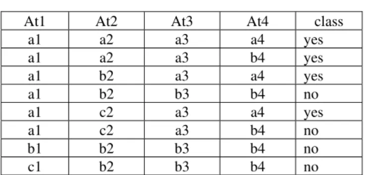
Decision trees are trees that classify instances by sorting them based on feature values. Each node in a decision tree represents a feature in an instance to be classified, and each branch represents a value that the node can assume. Instances are classified starting at the root node and sorted based on their feature values. An example of a decision tree for the training set of Table I.

Thair Nu Phyu is with University of Computer Studies, Pakokku, Myanmar (Email: Thair54@gmail.com)

Table I. Training set

At1 At2 At3 At4 class

a1 a2 a3 a4 yes

a1 a2 a3 b4 yes

a1 b2 a3 a4 yes

a1 b2 b3 b4 no

a1 c2 a3 a4 yes

a1 c2 a3 b4 no

b1 b2 b3 b4 no

c1 b2 b3 b4 no

Using the decision tree as an example, the instance At1 = a1, At2 = b2, At3 = a3, At4 = b4∗ would sort to the nodes: At1, At2, and finally At3, which would classify the instance as being positive (represented by the values “Yes”). The problem of constructing optimal binary decision trees is an NP complete problem and thus theoreticians have searched for efficient heuristics for constructing near-optimal decision trees.

The feature that best divides the training data would be the root node of the tree. There are numerous methods for finding the feature that best divides the training data such as information gain (Hunt et al., 1966) and gini index (Breiman et al., 1984). While myopic measures estimate each attribute independently, ReliefF algorithm (Kononenko, 1994) estimates them in the context of other attributes. However, a majority of studies have concluded that there is no single best method (Murthy,1998). Comparison of individual methods may still be important when deciding which metric should be used in a particular dataset. The same procedure is then repeated on each partition of the divided data, creating sub-trees until the training data is divided into subsets of the same class.

The basic algorithm for decision tree induction is a greedy algorithm that constructs decision trees in a top-down recursive divide-and-conquer manner. The algorithm, summarized as follows.

1. create a node N;

2. if samples are all of the same class, C then 3. return N as a leaf node labeled with the class C; 4. if attribute-list is empty then

5. return N as a leaf node labeled with the most common class in samples;

6. select test-attribute, the attribute among attribute-list with the highest information gain;

7. label node N with test-attribute; 8. for each known value ai of test-attribute

9. grow a branch from node N for the condition test-attribute= ai;

Survey of Classification Techniques in Data

Mining

10. let si be the set of samples for which test-attribute= ai;

11. if si is empty then

12. attach a leaf labeled with the most common class in samples;

13. else attach the node returned by

Generate_decision_tree(si,attribute-list_test-attribute) Fig.1 Algorithm for a decision tree

A decision tree, or any learned hypothesis h, is said to over fit training data if another hypothesis h2 exists that has a larger error than h when tested on the training data, but a smaller error than h when tested on the entire dataset. There are two common approaches that decision tree induction algorithms can use to avoid over fitting training data: i) Stop the training algorithm before it reaches a point at which it perfectly fits the training data, ii) Prune the induced decision tree. If the two trees employ the same kind of tests and have the same prediction accuracy, the one with fewer leaves is usually preferred. Breslow & Aha (1997) survey methods of tree simplification to improve their comprehensibility.

Decision trees are usually unvaried since they use based on a single feature at each internal node. Most decision tree algorithms cannot perform well with problems that require diagonal partitioning. The division f the instance space is orthogonal to the axis of one variable and parallel to all other axes. Therefore, the resulting regions after partitioning are all hyper rectangles. However, there are a few methods that construct multivariate trees. One example is Zheng’s(1998), who improved the classification accuracy of the decision trees by constructing new binary features with logical operators such as conjunction, negation, and disjunction. In addition, Zheng (2000) created at-least M-of-N features. For a given instance, the value of an at least M-of-N

representation is true if at least M of its conditions is true of the instance, otherwise it is false. Gama and Brazdil (1999) combined a decision tree with linear discriminate for constructing multivariate decision trees. In this model, new features are computed as linear combinations of the previous ones.

Decision trees can be significantly more complex representation for some concepts due to the replication problem. A solution is using an algorithm to implement complex features at nodes in order to avoid replication. Markovitch and Rosenstein (2002) presented the FICUS construction algorithm, which receives the standard input of supervised learning as well as a feature representation specification, and uses them to produce a set of generated features. While FICUS is similar in some aspects to other feature construction algorithms, its main strength is its generality and flexibility. FICUS was designed to perform feature generation given any feature representation specification complying with its general purpose grammar. The most well-know algorithm in the literature for building decision trees is the C4.5 (Quinlan, 1993). C4.5is an extension of Quinlan's earlier ID3 algorithm

(Quinlan, 1979). One of the latest studies that compare decision trees and other learning algorithms has been done by (Tjen-Sien Lim et al. 2000). The study shows that C4.5 has a very good combination of error rate and speed. In 2001, Ruggieri presented an analytic evaluation of the runtime behavior of the C4.5 algorithm, which highlighted some

efficiency improvements. Based on this analytic evaluation, he implemented a more efficient version of the algorithm, called EC4.5. He argued that his implementation computed the same decision trees asC4.5 with a performance gain of up to five times.

To sum up, one of the most useful characteristics of decision trees is their comprehensibility. People can easily understand why a decision tree classifies an instance as belonging to a specific class. Since a decision tree constitutes a hierarchy of tests, an unknown feature value during classification is usually dealt with by passing the example down all branches of the node where the unknown feature value was detected, and each branch outputs a class distribution. The output is a combination of the different class distributions that sum to 1. The assumption made in the decision trees is that instances belonging to different classes have different values in at least one of their features. Decision trees tend to perform better when dealing with discrete/categorical features.

3.BAYESIAN NETWORKS

A Bayesian Network (BN) is a graphical model for probability relationships among a set of variables features. The Bayesian network structure S is a directed acyclic graph (DAG) and the nodes in S are in one-to-one correspondence with the features X. The arcs represent casual influences among the features while the lack of possible arcs in S

encodes conditional independencies. Moreover, a feature (node) is conditionally independent from its non-descendants given its parents (X1 is conditionally independent from X2

given X3 if P(X1|X2,X3)=P(X1|X3) for all possible values of

X1, X2, X3).

Fig.2 The structure of Bayes network

Typically, the task of learning a Bayesian network can be divided into two subtasks: initially, the learning of the DAG structure of the network, and then the determination of its parameters. Probabilistic parameters are encoded into a set of tables, one for each variable, in the form of local conditional distributions of a variable given its parents. Given the independences encoded into the network, the joint distribution can be reconstructed by simply multiplying these tables. Within the general framework of inducing Bayesian networks, there are two scenarios: known structure and unknown structure.

Conditional Probability Tables (CPT) is usually solved by estimating a locally exponential number of parameters from the data provided (Jensen, 1996). Each node in the network has an associated CPT that describes the conditional probability distribution of that node given the different values of its parents. In spite of the remarkable power of Bayesian Networks, they have an inherent limitation. This is the computational difficulty of exploring a previously unknown network. Given a problem described by n features, the number of possible structure hypotheses is more than exponential in n. If the structure is unknown, one approach is to introduce a scoring function (or a score) that evaluates the “fitness” of networks with respect to the training data, and then to search for the best network according to this score. Several researchers have shown experimentally that the selection of a single good hypothesis using greedy search often yields accurate predictions (Heckerman et al. 1999), (Chickering, 2002).

The most interesting feature of BNs, compared to decision trees or neural networks, is most certainly the possibility of taking into account prior information about a given problem, in terms of structural relationships among its features. This prior expertise, or domain knowledge, about the structure of a Bayesian network can take the following forms:

1. Declaring that a node is a root node, i.e., it has no parents.

2. Declaring that a node is a leaf node, i.e., it has no children.

3. Declaring that a node is a direct cause or direct effect of another node.

4. Declaring that a node is not directly connected to another node.

5. Declaring that two nodes are independent, given a condition-set.

6. Providing partial nodes ordering, that is, declare that a node appears earlier than another node in the ordering.

7. Providing a complete node ordering.

A problem of BN classifiers is that they are not suitable for datasets with many features (Cheng et al., 2002). The reason for this is that trying to construct a very large network is simply not feasible in terms of time and space. A final problem is that before the induction, the numerical features need to be discredited in most cases.

4. K-NEAREST NEIGHBOR CLASSIFIERS Nearest neighbor classifiers are based on learning by analogy. The training samples are described by n dimensional numeric attributes. Each sample represents a point in an n-dimensional space. In this way, all of the training samples are stored in an n-dimensional pattern space. When given an unknown sample, a k-nearest neighbor classifier searches the pattern space for the k training samples that are closest to the unknown sample. "Closeness" is defined in terms of Euclidean distance, where the Euclidean distance, where the Euclidean distance between two points, X=(x1,x2,……,xn) and Y=(y1,y2,….,yn) is

d(X, Y)= 2

1

)

(

n

i

i

y

x

−

∑

=

The unknown sample is assigned the most common class among its k nearest neighbors. When k=1, the unknown sample is assigned the class of the training sample that is closest to it in pattern space.

Nearest neighbor classifiers are instance-based or lazy learners in that they store all of the training samples and do not build a classifier until a new(unlabeled) sample needs to be classified. This contrasts with eager learning methods, such a decision tree induction and backpropagation, which construct a generalization model before receiving new samples to classify. Lazy learners can incur expensive computational costs when the number of potential neighbors (i.e.,stored training samples)with which to compare a given unlabeled smaple is great. Therefore, they require efficient indexing techniques. An expected lazy learning methods are faster ata trainging than eager methods, but slower at classification since all computation is delayed to that time. Unlike decision tree induction and backpropagation, nearest neighbor classifiers assign equal weight to each attribute. This may cause confusion when there are many irrelevant attributes in the data.

Nearest neighbor classifiers can also be used for prediction, that is, to return a real-valued prediction for a given unknown sample. In this case, the classifier retruns the average value of the real-valued associated with the k neraest neighbors of the unknown sample.

The k-nearest neighbors’ algorithm is amongest the simplest of all machine learning algorithms. An object is classified by a majority vote of its neighbors, with the object being assigned to the class most common amongst its k

nearest neighbors. k is a positive integer, typically small. If k

= 1, then the object is simply assigned to the class of its nearest neighbor. In binary (two class) classification problems, it is helpful to choose k to be an odd number as this avoids tied votes.

The same method can be used for regression, by simply assigning the property value for the object to be the average of the values of its k nearest neighbors. It can be useful to weight the contributions of the neighbors, so that the nearer neighbors contribute more to the average than the more distant ones.

The neighbors are taken from a set of objects for which the correct classification (or, in the case of regression, the value of the property) is known. This can be thought of as the training set for the algorithm, though no explicit training step is required. In order to identify neighbors, the objects are represented by position vectors in a multidimensional feature space. It is usual to use the Euclidian distance, though other distance measures, such as the Manhanttan distance could in principle be used instead. The k-nearest neighbor algorithm is sensitive to the local structure of the data.

4.1 INSTANCE-BASED LEARNING

classification process. One of the most straightforward instance-based learning algorithms is the nearest neighbor

algorithm. Aha (1997) and De Mantaras and Armengol (1998) presented a review of instance-based learning classifiers. Thus, in this study, apart from a brief description of the nearestneighbor algorithm, we will refer to some more recent works. k-Nearest Neighbor (kNN) is based on the principle that the instances within a dataset will generally exist in close proximity to other instances that have similar properties (Cover and Hart, 1967). If the instances are tagged with a classification label, then the value of the label of an unclassified instance can be determined by observing the class of its nearest neighbors. The Knn locates the k nearest instances to the query instance and determines its class by identifying the single most frequent class label. In Figure 8, a pseudo-code example for the instance base learning methods is illustrated.

procedure InstanceBaseLearner(Testing Instances)

for each testing instance {

find the k most nearest instances of the training set according to a distance metric

Resulting Class= most frequent class label of the k nearest instances }

Fig.3 Pseudo-code for instance-based learners In general, instances can be considered as points within an

n-dimensional instance space where each of the

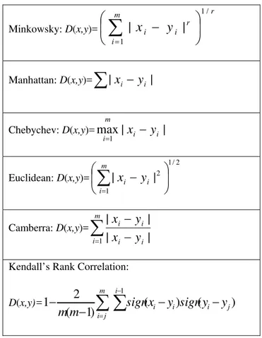
n-dimensions corresponds to one of the n-features that are used to describe an instance. The absolute position of the instances within this space is not as significant as the relative distance between instances. This relative distance is determined by using a distance metric. Ideally, the distance metric must minimize the distance between two similarly classified instances, while maximizing the distance between instances of different classes. Many different metrics have been presented. The most significant ones are presented in Table II.

For more accurate results, several algorithms use weighting schemes that alter the distance measurements and voting influence of each instance. A survey of weighting schemes is given by (Wettschereck et al., 1997). The power of kNN has been demonstrated in a number of real domains, but there are some reservations about the usefulness of kNN, such as: i) they have large storage requirements, ii) they are sensitive to the choice of the similarity function that is used to compare instances, iii) they lack a principled way to choose k, except through cross-validation or similar, computationally-expensive technique (Guo et al. 2003). The choice of k affects the performance of the Knn algorithm. Consider the following reasons why a knearest neighbour classifier might incorrectly classify a query instance:

฀ When noise is present in the locality of the query instance; the noisy instance(s) win the majority vote, resulting in the

incorrect class being predicted. A larger k could solve this problem.

When the region defining the class, or fragment of the class, is so small that instances belonging to the class that surrounds the fragment win the majority vote. A smaller k

could solve this problem.

Table II. Approaches to define the distance between instances (x and y)

Minkowsky: D(x,y)=

r m

i

r i

i

y

x

/ 1

1

|

|

⎟

⎠

⎞

⎜

⎝

⎛

₋

∑

=

Manhattan: D(x,y)=

∑

|

x

−

y

|

Chebychev: D(x,y)=

max

|

|

1 i i

m

i=

x

−

y

Euclidean: D(x,y)=

2 / 1 2

1

|

|

⎟

⎠

⎞

⎜

⎝

⎛

₋

∑

=

m

i

i i

y

x

Camberra: D(x,y)=

∑

=

−

−

m

i i i i i

y

x

y

x

1

|

|

|

|

Kendall’s Rank Correlation:

D(x,y)=

(

)

(

)

)

1

(

2

1

1

j i i i

i m

j i

y

y

sign

y

x

sign

m

m

−

−

−

−

∑

∑

=

Wettschereck et al. (1997) investigated the behavior of the kNN in the presence of noisy instances. The experiments showed that the performance of kNN was not sensitive to the exact choice of k when k was large. They found that for small values of k, the kNN algorithm was more robust than the single nearest neighbor algorithm (1NN) for the majority of large datasets tested. However, the performance of the kNN was inferior to that achieved by the 1NN on small datasets (<100 instances).

Okamoto and Yugami (2003) represented the expected classification accuracy of k-NN as a function of domain characteristics including the number of training instances, the number of relevant and irrelevant attributes, the probability of each attribute, the noise rate for each type of noise, and k. They also explored the behavioral implications of the analyses by presenting the effects of domain characteristics on the expected accuracy of k-NN and on the optimal value of k for artificial domains.

reduction algorithm is to modify the instances using a new representation such as prototypes (Sanchez et al., 2002). Breiman (1996) reported that the stability of nearest neighbor classifiers distinguishes them from decision trees and some kinds of neural networks. A learning method is termed "unstable" if small changes in the training-test set split can result in large changes in the resulting classifier.

As we have already mentioned, the major disadvantage of instance-based classifiers is their large computational time for classification. A key issue in many applications is to determine which of the available input features should be used in modeling via feature selection (Yu & Liu, 2004), because it could improve the classification accuracy and scale down the required classification time. Furthermore, choosing a more suitable distance metric for the specific dataset can improve the accuracy of instance-based classifiers.

5. CONCLUSION

Decision trees and Bayesian Network (BN) generally have different operational profiles, when one is very accurate the other is not and vice versa. On the contrary, decision trees and rule classifiers have a similar operational profile. The goal of classification result integration algorithms is to generate more certain, precise and accurate system results. Numerous methods have been suggested for the creation of ensemble of classifiers. Although or perhaps because many methods of ensemble creation have been proposed, there is as yet no clear picture of which method is best.

Classification methods are typically strong in modeling interactions. Several of the classification methods produce a set of interacting loci that best predict the phenotype. However, a straightforward application of classification methods to large numbers of markers has a potential risk picking up randomly associated markers.

R

[1] Baik, S. Bala, J. (2004), A Decision Tree Algorithm for Distributed Data Mining: Towards Network Intrusion Detection, Lecture Notes in Computer Science, Volume 3046, Pages 206 – 212.

[2] Bouckaert, R. (2004), Naive Bayes Classifiers That Perform Well with Continuous Variables, Lecture Notes in Computer Science, Volume 3339, Pages 1089 – 1094.

[3] Breslow, L. A. & Aha, D. W. (1997). Simplifying decision trees: A survey. Knowledge EngineeringReview 12: 1–40. [4] Brighton, H. & Mellish, C. (2002), Advances in Instance

Selection for Instance-Based Learning Algorithms. Data Mining and KnowledgeDiscovery 6: 153–172.

[5] Cheng, J. & Greiner, R. (2001). Learning Bayesian Belief Network Classifiers: Algorithms and System, In Stroulia, E. & Matwin, S. (ed.), AI 2001, 141-151, LNAI 2056,

[6] Cheng, J., Greiner, R., Kelly, J., Bell, D., & Liu, W. (2002). Learning Bayesian networks from data: An information-theory based approach. ArtificialIntelligence 137: 43–90.

[7] Clark, P., Niblett, T. (1989), The CN2 Induction Algorithm. Machine Learning, 3(4):261-283.

[8] Cover, T., Hart, P. (1967), Nearest neighbor pattern classification. IEEE Transactions on Information Theory, 13(1): 21–7.

[9] Cowell, R.G. (2001). Conditions Under Which Conditional Independence and Scoring Methods Lead to Identical Selection

of Bayesian Network Models. Proc. 17th International Conference on Uncertainty in Artificial Intelligence.

[10] Domingos, P. & Pazzani, M. (1997). On the optimality of the simple Bayesian classifier under zero-one loss. Machine Learning 29: 103-130.

[11] Elomaa T. (1999). The biases of decision tree pruning strategies. Lecture Notes in Computer Science 1642. Springer, pp. 63-74.

[12] Friedman, N., Geiger, D. & Goldszmidt M. (1997). Bayesian network classifiers. Machine Learning 29: 131-163.

[13] Friedman, N. & Koller, D. (2003). Being Bayesian About Network Structure: A Bayesian Approach to Structure Discovery in Bayesian Networks. Machine Learning 50(1): 95-125.

[14] Jensen, F. (1996). An Introduction to Bayesian Networks. Springer.

[15] Kubat, Miroslav Cooperson Martin (2001), A reduction technique for nearest-neighbor classification: Small groups of examples. Intell. Data Anal. 5(6): 463-476.

[16] Madden, M. (2003), The Performance of Bayesian Network Classifiers Constructed using Different Techniques, Proceedings of European Conference on Machine Learning, Workshop on Probabilistic Graphical Models for Classification, pp. 59-70.

[17] McSherry, D. (1999). Strategic induction of decision trees. Knowledge-Based Systems, 12(5- 6):269-275.

[18] Vivarelli, F. & Williams, C. (2001). Comparing Bayesian neural network algorithms for classifying segmented outdoor images. Neural Networks 14: 427-437.

[19] Wilson, D. R. & Martinez, T. (2000). Reduction Techniques for Instance-Based Learning Algorithms. Machine Learning 38: 257–286.

[20] Witten, I. & Frank, E. (2005), "Data Mining: Practical machine learning tools and techniques", 2nd Edition, Morgan Kaufmann, San Francisco, 2005.

[21] Yang, Y., Webb, G. (2003), On Why Discretization Works for Naive-Bayes Classifiers, Lecture Notes in Computer Science, Volume 2903, Pages 440 – 452.

[22] Zhang, G. (2000), Neural networks for classification: a survey. IEEE Transactions on Systems, Man, and Cybernetics, Part C 30(4): 451- 462.