UNIVERSIDADE DE ÉVORA
DEPARTAMENTO DE ECONOMIA
DOCUMENTO DE TRABALHO Nº 2005/11
June
Bias-corrected Moment-based Estimators for
Parametric Models under Endogenous Stratified Sampling
Joaquim J. S. Ramalho*
Universidade de Évora, Departamento de Economia, CEMAPRE
Esmeralda A. Ramalho
Universidade de Évora, Departamento de Economia, CEMAPRE
* The authors gratefully acknowledge partial financial support from Fundação para a Ciência e Tecnologia, program POCTI, partially funded by FEDER. Address for correspondence: Esmeralda A. Ramalho, Department of Economics, Universidade de Évora, 7000-803 ÉVORA, Portugal (email: [email protected]).
UNIVERSIDADE DE ÉVORA
DEPARTAMENTO DE ECONOMIA
Largo dos Colegiais, 2 – 7000-803 Évora – Portugal Tel.: +351 266 740 894 Fax: +351 266 742 494 www.decon.uevora.pt [email protected]
Abstract:
This paper provides an integrated approach for estimating parametric models from endogenous stratified samples. We discuss several alternative ways of removing the bias of the moment indicators usually employed under random sampling for estimating the parameters of the structural model and the proportion of the strata in the population. Those alternatives give rise to a bunch of moment-based estimators which are appropriate for both cases where the marginal strata probabilities are known and unknown. The derivation of our estimators is very simple and intuitive and incorporates as particular cases most of the likelihood-based estimators existing in the literature.
Palavras-chave/Keywords: Endogenous Stratified Sampling, Bias correction, GMM, Parametric
models
1
Introduction
In many research settings, economists are often interested in estimating parametric models based on endogenously stratified samples (ESS), where the probability of be-ing sampled depends on the value of the variable of interest. In contrast to random or exogenously stratified samples, with ESS the marginal distribution of the covariates does not factor out from the likelihood of the observed data, so, unless that distrib-ution is known, nonstandard estimation procedures are required to handle correctly the data. The most well known estimators in this area result from likelihood-based approaches which circumvent the formalization of the marginal distribution of the covariates and only require, as usual, the specification of the conditional distribution of the variable of interest given the covariates; see, for example, Manski and Lerman (1977), Manski and McFadden (1981), Cosslett (1981a,b), and Imbens (1992), who propose estimators for the particular case of choice-based samples (the stratifica-tion is based on the discrete values of the dependent variable, which often represent choices), and Imbens and Lancaster (1996), who address the general case of ESS. While the estimators proposed in the two first papers require the availability of exact information on the strata probabilities in the population, the others are also appropriate for the case where those probabilities are unknown.
Despite their wider potential usefulness for applied researchers, to the best of our knowledge, none of the estimators developed by Cosslett (1981a,b), Imbens (1992), and Imbens and Lancaster (1996) has ever been used in empirical work. In ef-fect, perhaps intimidated by the complex theoretical derivations of those estimators, practitioners seem to prefer assuming that the proportions of the strata in the pop-ulation are exactly known, using census or similar information, which allows them to apply the much simpler Manski and Lerman’s (1977) weighted maximum like-lihood (WML) or Manski and McFadden’s (1981) conditional maximum likelike-lihood (CML) methods (e.g. Artis, Ayuso and Guillen, 1999, Early, 1999, and Kitamura, Yamamoto Sakai, 2003). While in some cases that assumption is admissible, in others it may lead to biased estimates (if there are important differences between the estimated and the actual population strata probabilities) or underestimation of
standard errors (if the information available on the population probabilities of the strata is not exact). Moreover, even when the available information on the popula-tion strata probabilities is in fact correct, both the WML and the CML estimators are not the best choice since they are not as efficient as Cosslett (1981a,b), Imbens (1992), and Imbens and Lancaster’s (1996) estimators.
In this paper we develop a moment-based framework for estimating paramet-ric models under ESS. Our estimators are based on bias-corrected versions of two types of moment conditions which are valid under random sampling (RS): the score functions usually employed for estimating the parameters of the structural model; and a set of equations defining the population strata probabilities. Two alternative principles are applied to correct the moment conditions in order to guarantee that their expectation under the distribution of the data is zero. The first builds on the idea of Manski and Lerman (1977) of reweighting each observation in such a way that the structure of the target population is reconstructed by reducing (increasing) in an appropriate manner the weight of oversampled (undersampled) strata. The second, in the spirit of Manski and McFadden (1981), consists of subtracting from each moment condition its bias under ESS. In both cases, the resulting moment con-dition model may be estimated by Hansen’s (1982) generalized method of moments (GMM) or any of the generalized empirical likelihood methods recently discussed by Newey and Smith (2004).
These alternative simple corrections may be combined in a number of different ways, giving rise to a bunch of alternative estimators, which may be employed both when the marginal strata probabilities in the population are known and unknown. As may be inferred from the discussion above, our estimators may be interpreted as generalizations of Manski and Lerman (1977) and Manski and McFadden’s (1981) estimators. They also encompass as particular cases most of Cosslett (1981a,b), Imbens (1992), and Imbens and Lancaster (1996) estimators. However, in contrast to them, our integrated approach is very simple and intuitive and, hopefully, will encourage practitioners to choose the most adequate estimators in each particular empirical analysis.
charac-teristics of ESS. Section 3 derives some bias-corrected moment conditions which are valid under ESS. Section 4 discusses how those moment conditions may be used to give rise to alternative moment-based estimators. Section 5 compares our estimators with those referred to above. Section 6 is dedicated to a Monte Carlo investigation of the finite sample properties of most of the estimators discussed throughout the paper. Finally, section 7 concludes.
2
Endogenous stratified samples
Consider a sample of i = 1, ..., N individuals and let Y be the variable of interest, continuous or discrete, and X a vector of k exogenous variables. Both Y and X are random variables defined on Y × X with population joint density function
f (y,x; θ) = f (y|x, θ) f (x) , (1)
where the conditional density function f (y|x, θ) is known up to the parameter vector θ and the marginal density function f (x) is unknown. Our interest is estimation of and inference on the parameter vector θ in f (y|x, θ).
ESS involves the partition of the population into strata, which are defined accord-ing to the values taken by Y . Assume the existence of J non-empty and possibly overlapping strata, which are subsets of Y × X . Each stratum is designated as Cs =Ys× X , with S ∈ S = {1, ..., J}, and Ys is defined as the subset of Y for which
the observation (Y, X) lies in Cs. The proportion of stratum Cs in the population is
given by Qs(θ) = Z Ys Z X f (y,x; θ) dxdy, (2)
where Qs(θ) > 0 and, in case of mutually exclusive strata, Ps∈SQs(θ) = 1. To
simplify the notation we define Qs ≡ Qs(θ).
One of the mechanisms which may be employed for drawing an ESS is the so-called multinomial sampling. In this sampling scheme, considered, for example, by Manski and Lerman (1977), Manski and McFadden (1981), and Imbens (1992), it is assumed that the stratum indicators S are drawn independently from a multinomial
distribution. The sampling agent randomly selects a stratum Cs with a pre-defined
probability Hs, where Hs > 0 and Ps∈SHs = 1, and, then, randomly samples
from that stratum.1 In this setting, the variable of interest, the covariates, and the stratum indicator are observed according to
h (z) = bsf (y|x, θ) f (x) , (3) where Z = (Y, X, S), Q0 ≡ [Q 1, ..., QJ] is a J-vector, and2 bs = Hs Qs . (4)
On the other hand, the sampling distribution of X is given by
h (x) = X s∈S Z Ys h (z) dy = bxf (x), (5) where bx = X s∈S bs Z Ys f (y|x, θ) dy. (6) Both bs and bx may be interpreted as bias functions, reflecting the bias induced
by ESS over the population density functions f (y,x; θ), in the former case, and f (x),
in the latter. These distortions are eliminated only when the ESS is obtained by self-weighting (Hs = Qs), in which case bs = bx = 1. Due to the presence of bs in
(3), maximum likelihood (ML) estimation of θ requires the specification of f (x), since this density is contained in bs via Qs; see equations (2) and (4). For this
reason, and also because the bias bx that is present in (5) is a function of θ, X is
not exogenous for this parameter, which means that conditioning on it produces a
1Although its relevancy in practice may be questionable, in this paper we will deal with
multino-mial sampling because it generates a simple setup and, more important, it is observationally equiv-alent to the two sampling schemes more popular in applied work, the so-called standard stratified and variable probability sampling schemes; see Imbens and Lancaster (1996) for a discussion on these alternative sampling schemes.
2Note that, in case of non-overlapping strata, as Q
J = 1 −
J−1
X
s=1
Qs, only the J − 1-vector
loss of information on θ. Therefore, all the estimation procedures suggested in this paper are based on expectations taken with respect to the joint density function h (z)but circumvent the need for specifying f (x).
The bias functions (4) and (6) have some interesting properties, which will be ex-ploited later on in the derivation of the bias-corrected estimating functions. Namely,
E¡b−1s ¢= E¡b−1x ¢ = 1, (7) E · b−1s Z Yt f (y|x, θ) dy ¸ = E · b−1x Z Yt f (y|x, θ) dy ¸ = Qt, for t = 1, ..., J , (8) EX · bx Z Yt f (y|x, θ) dy ¸ = E · b−1s bx Z Yt f (y|x, θ) dy ¸ (9) and EX(∇θbx) = E ¡ b−1x ∇θbx ¢ , (10)
where ∇θm (θ) = ∂m (θ)/ ∂θ and E (·) and EX(·) denote expectation taken with
respect to h (z) and f (x), respectively; see the derivations in the Appendix.
3
Moment conditions for parametric models
un-der ESS
The moment-based estimators proposed in this paper are based on bias-corrected versions of the estimating functions defining θ and Q under RS. In this section we start by deriving the bias of those functions under ESS, then we discuss two alternative methods for adjusting them in order to eliminate their bias, and finally we introduce a further moment condition that allows more efficient estimators to be obtained.
3.1
The bias of the estimating functions defining
θ and Q
under random sampling
Under RS, all the analysis may be conditional on X, so the relevant log-likelihood function for estimation of θ is simply
L (θ) =
n
X
1=1
ln f (yi|xi, θ), (11)
which implies that the ML estimator for θ may be defined as the solution to the sampling counterpart of the set of equations
EY |X [g (θ)RS] = 0, (12)
where g (θ)RS ≡ ∇θln f (y|x, θ) and EY |X [·] denotes expectation taken with respect
to f (y |x, θ ). However, under ESS, as the observed data are described by h (z) of (3), the relevant expectation of g (θ)RS is taken with respect to h (z), being given by
E [g (θ)RS] = X s∈S Z Ys Z X ∇θf (y|x, θ) f (y|x, θ) bsf (y|x, θ) f (x) dydx = Z X X s∈S bs Z Ys ∇θf (y|x, θ) f (x) dydx = EX(∇θbx), (13)
which is not zero in general.
On the other hand, from (2), a consistent estimator for Qt, t = 1, ..., J , under
RS is ˆ Qt= 1 N N X i=1 Z Yt f³yi|xi, ˆθ ´ dy, (14)
which results from solving the sampling counterpart of
EY |X [g (Qt)RS] = 0, (15)
where g (Qt)RS ≡ Qt−
R
respect to h (z) is not zero but E [g (Qt)RS] = Qt− Z X X s∈S Z Ys Z Yt f (y|x, θ) dybs(Q) f (y|x, θ) f (x) dydx = Qt− Z X X s∈S bs Z Ys f (y|x, θ) dy Z Yt f (y|x, θ) dyf (x) dx = Qt− Z X bx Z Yt f (y|x, θ) f (x) dydx = Qt− EX ·Z X bx Z Yt f (y|x, θ) dy ¸ . (16)
Naturally, unless the sampling is self-weighting, in which case, as bx = 1 and
∇θbx = 0, expectations (13) and (16) are zero, imposing (12) and (15) in the sample
yields inconsistent estimators for θ and Q.
3.2
Bias-adjusted moment conditions
The RS estimating functions (12) and (15) may be adjusted in order to produce consistent estimators for θ and Q also under ESS. The analysis of the estimating functions for θ proposed in the pioneering works of Manski and Lerman (1977) and Manski and McFadden (1981) suggests two alternative ways of correcting the estimating functions for RS. The first consists of reweighting each observation in such a way that the population structure is reconstructed. The second involves subtracting a term to the RS estimating functions, such that the expectations of their modified versions are zero. Thus, the parameters of the structural model θ may be consistently estimated from the weighted moment indicators
g1(θ) = b−1s g (θ)RS. (17)
or, alternatively, using results (10) and (13), we may employ the modified estimating functions
g2(θ) = g (θ)RS − b−1s ∇θbx. (18)
The same approach used to obtain (17) and (18) may be followed to derive estimating functions for Q. We derive four different modifications of g (Qt)RS of the
type proposed by Manski and Lerman (1977), all of them based on results (7) and (8). In fact, g (Qt)RS may be simply weighted by the inverse of the biases (4) and
(6), which yields,
ga(Qt) = b−1s g (Qt)RS (19)
and
gb(Qt) = b−1x g (Qt)RS, (20)
t = 1, ..., J. Alternatively, see (8), only the second term of g (Qt)RS is weighted,
which gives rise to
gc(Qt) = Qt− b−1s Z Yt f (y|x, θ) dy (21) and gd(Qt) = Qt− b−1x Z Yt f (y|x, θ) dy. (22) On the other hand, to construct a Manski and McFadden (1981)-type of bias-adjusted moment indicators, we propose the subtraction of the term Qt−b−1s bx
R
Ytf (y|x, θ) dy,
whose expectation equals that of g (Qt)RS, see equations (9) and (16), to this
esti-mating function. The resulting moment indicators are
ge(Qt) = ¡ b−1s bx− 1 ¢ Z Yt f (y|x, θ) dy. (23)
In all cases, it is straightforward to show that the expectations of (17)-(23) taken with respect to h (z) are zero. Moreover, consistent estimators for those expectations may be straightforwardly obtained since the empirical distribution function is the nonparametric likelihood estimator of the distribution function based on h (z).
3.3
Moment conditions for
H
sAlthough not essential for obtaining consistent estimators for θ and Q under ESS, Imbens (1992) stressed the importance of conditioning the analysis on the ancillary statistics ˆHs = Ns/N, where Ns is the number of individuals included in stratum
of the set of (J − 1) moment indicators3
g (Ht) = Ht− 1 (s = t) , t = 1, ..., J− 1 (24)
to estimate the vector H0 ≡ [H1, ..., HJ −1]; see Imbens (1992) and Imbens and
Lancaster (1996) for a comprehensive discussion on this issue.
4
Moment-based estimators
Efficient estimators for θ and Q can be obtained by using in an appropriate manner the bias-corrected moment indicators derived in the previous section. According to the way the bias-corrected moment indicators are combined, different will be the resulting moment-based estimator. In this section we analyze the main alternatives.
4.1
Alternative moment condition models
All the information regarding the bias-corrected moment indicators can be summa-rized as
E [g (β0)] = 0, (25)
where β0 denotes the true value of the vector of parameters of interest β and g (·)
is a vector of moment indicators. The specific composition of β and g (β) depends on several factors, which are discussed next.
In case the population strata probabilities are unknown, or the available aggre-gate figures on Q do not seem to be reliable, β0 ≡ (θ0, Q0, H0) is a (k + 2J − 1)-dimensioned vector of parameters of interest, and g (β) comprises the k-vector g (θ) [defined as g1(θ) or g2(θ)], the J-vector g (Q) [defined as ga(Q), gb(Q), gc(Q),
gd(Q), or ge(Q)], and the (J − 1)-vector g (H). In the opposite case of exact
knowl-edge on Q, we can still use g (β)0 ≡£g (θ)0, g (Q)0, g (H)0¤but now Q is replaced by its known value and only the (k + J − 1) vector β0 ≡ (θ0, H0)needs to be estimated.
Therefore, this second case gives rise to an overidentifying system of equations.
3Note that an estimating function for H
Note that only the estimators based on moment indicators which are equivalent to the scores of a likelihood function based on the sampling density function of (y, x, s) or (y, x) given s, i.e. based on g (β)0 ≡ £g2(θ)0, gb(Q)0, g (H)0
¤
or g (β)0 ≡ £
g2(θ)0, gd(Q)0, g (H)0
¤
, are efficient. Other consistent but inefficient estimators are those based solely on g (θ)0 or£g (θ)0, g (H)0¤(Q known), or g (β)0 ≡£g (θ)0, g (Q)0¤. However, here the loss of precision is due to the suppression of moment indicators for Q and/or H in the estimation.
4.2
GMM estimation
Various methods of estimation may be used for estimating the model specified by the moment conditions (25). The standard method is the GMM, see Hansen (1982). Let ˆg(β) ≡ PNi=1g(zi, β)
.
N and ˆW denote a symmetric, positive definite matrix that converges almost surely to a nonrandom, positive definite matrix W . When the number of moment conditions and unknown parameters is identical, an efficient GMM estimator is defined by
ˆ
β = arg min
β∈Bˆg(β)
0Wˆ−1g(β),ˆ (26)
where B denotes the parameter space. On the other hand, in the overidentifying case a two-step efficient GMM estimator is given by
ˆ β = arg min β∈Bg(β)ˆ 0Ω(˜ˆ β)−1g(β),ˆ (27) where ˆΩ(β)≡ PNi=1gi(β)gi(β)0 .
N and ˜β is some preliminary estimator defined by an equation similar to (26).
Under suitable regularity conditions, see Newey and McFadden (1994), we have in both cases
√
N³βˆ− β0
´ d
→ Nh0,¡G0Ω−1G¢−1i, (28) where→ denotes convergence in distribution, G ≡ E [∇d βg(β)], and Ω ≡ E [g(z, β)g(z, β)0].
Alternative estimation methods which share the first order asymptotic properties of GMM are those in the generalized empirical likelihood (GEL) class. However, as
often they are computationally more evolving, and in the just identified case they yield estimates numerically identical to GMM, in this paper we only consider GMM estimation. See Newey and Smith (2004) for more details on GEL estimation.
5
Comparison with other estimators
Among the several estimators produced by our methodology are most of the likelihood-based estimators proposed previously by other authors. Indeed, the estimators sug-gested by Manski and Lerman (1977), Manski and McFadden (1981), Imbens (1992), Imbens and Lancaster (1996), and, only for unknown Q, Cosslett (1981a,b) may be obtained as GMM estimators defined by (26) or (27). The only aspect that dif-ferentiates them is the composition of the vectors β and g (β) in (25), as we show below.
As most estimators were derived for the particular case of choice-based samples (CBS), ESS where the variable of interest takes values on a set of (C + 1) mutually exclusive alternatives, Y ∈ {0, 1, ..., C}, some notational modifications need to be done to simplify the comparisons. First, due to the discrete nature of the variable of interest, f (y|x, θ) must be replaced by Pr (y|x, θ) and integration over Ys is
sub-stituted by summation. Second, we may define the sampling and the population probability of observing an individual choosing Y = y as, respectively, Hy and Qy =
R XPr (y|x, θ) f (x) dx, 0 < Hy < 1, 0 < Qy < 1, P y∈YsHy = 1, and P y∈YsQy = 1, and write Hs = P y∈YsHy, Qs = P y∈YsQy, and bx = P y∈Y Hy Qy Pr (y|x, θ). Of
course, when each choice defines one stratum such that Cs = Y × X and Y = S, a
sampling scheme which we designate here as pure CBS, the notation may be further simplified, since Qs = Qy, Hs= Hy, and the stratum indicator S may be suppressed.
5.1
Manski and Lerman (1977) and Manski and McFadden’s
(1981) estimators
Manski and Lerman (1977) and Manski and McFadden (1981) derived modified ML estimators for pure CBS for the case where exact information on the marginal probability Qy is available. In both cases, β = θ since they work with the true values
of Qy and Hy. These estimators are numerically identical to the GMM estimators
(26) based on g (β) = g1(θ) and g (β) = g2(θ), respectively. Our framework shows
clearly that both Manski and Lerman (1977) and Manski and McFadden’s (1981) estimators are consistent but not efficient, since the moment indicators g (Q) and g (H)are omitted from g (β), and provides a simple way of extending both estimators for the general case of ESS and for unknown Qy.
5.2
Imbens (1992) and Imbens and Lancaster’s (1996)
esti-mators
Imbens (1992) and Imbens and Lancaster (1996) proposed efficient GMM estimators for, respectively, CBS and ESS, both of which are based on the set of moment indicators g (β)0 ≡£g2(θ)0, gd(Q)0, g (H)0
¤
. These authors considered both the cases where Q is known or otherwise, so the vector of parameters of interest is β0 = (θ0, H0) or β0 = (θ0, Q0, H0), respectively. Note that the approach we followed in this
paper has two advantages relatively to theirs. First, the derivation of our estimators was incomparably simpler since from the start they are typical GMM estimators. In contrast, the theoretical derivations made by Imbens (1992) and Imbens and Lancaster (1996) are much more complex, involving the assumption of a discrete distribution for the covariates, which is in an initial step jointly estimated with the parameters of interest, and the concentration of the log-likelihood h (z) of (3) with respect to the mass point probabilities of X. Second, our method gives rise to many other alternative estimators by combining in different ways the vectors (17)-(23).
5.3
Cosslett’s (1981a,b) estimators
Like Imbens (1992), Cosslett (1981a,b) proposed efficient estimators for CBS. How-ever, in contrast to Imbens (1992), the estimator suggested by Cosslett (1981a) for the case where Q is known differs markedly from the case where Q is unknown. As we show now, the estimator developed for the latter case is also a particular case of our estimators, although the comparison is not so straightforward as in the previous cases, for two reasons. First, Cosslett (1981a,b) assumes that the sample is
gathered by standard stratified sampling, a sampling scheme where instead of fixing Hs, as in multinomial sampling, the sampling agent fixes Ns. Hence, instead of Hs,
which is now unknown, the term Ns/N appears explicitly in the likelihood function
to be maximized, so the analysis is automatically based on the ancillary statistics ˆ
Hs = Ns/N. Second, instead of Q, Cosslett (1981a,b) suggests the estimation of a
(J− 1)-dimensional vector of auxiliary parameters λs = ˆHs/Qs, λ = (λ1, λ2, ...,
λJ−1).
In order to estimate the parameters of interest (θ, λ), Cosslett (1981a,b) proposes the maximization of the pseudo log-likelihood function
L (θ, λ) = N X i=1 ln " λsiPr (yi|xi, θ) P s∈S P y∈YsλsPr (y|x, θ) # , subject to λs≥ 0 and PJ
s=1λs= 1. If we derive this function with respect to θ and
λ, we obtain two score functions which are given by, respectively, g2(θ) and gb(Q)
with bs replaced by λs and Qt of gb(Q) replaced by ˆ Ht
λt, which shows, clearly, that
this estimator may also be seen as a particular case of ours.
6
Monte Carlo simulation study
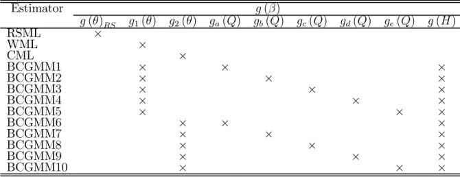
To investigate the performance in finite samples of the bias-corrected GMM (BCGMM) estimators discussed in this paper, we carried out two distinct Monte Carlo analy-sis. First, we replicated the examples of stratified sampling in the normal linear model analyzed by Imbens and Lancaster (1996). Then, based on some of Cosslett’s (1981) designs, we considered some particular examples of endogenous stratification in Probit models. In both cases, we computed 13 different estimators, as described in Table 1: the conventional RS maximum likelihood (RSML) estimator, which is inconsistent in all cases simulated, the popular WML and CML estimators, and 10 alternative BCGMM estimators. In the Appendix we present the moment indicators associated to each estimator specialized to the models simulated.
For each estimator we report the mean and median bias, the standard error (SE) across replications, and the root mean square error (RMSE). All experiments were based on samples of N = 200 and 5000 replications.
6.1
Normal linear model
Similarly to Imbens and Lancaster (1996), we consider a normal linear model defined by y = α0+ α1x + , |x ∼ N ¡ 0, σ2¢, that is f (y|x, θ) = σ1φ ¡y−α0−α1x σ ¢
, where θ = (α0, α1, σ2). We generated enriched
samples which combine a stratum corresponding to a RS, designated as stratum 0, with one stratum including individuals for which the value of Y is larger than a cut-off point C, designated as stratum 1. The proportion of each stratum in the population is, respectively, 1 and Q. Four different combinations of cut-off points, values for θ, and distributions for X were considered in order to produce different proportions Q; see Table 2. In the four examples, the sampling proportions of both strata are equal, i.e. H0 = H1 = H = 0.5.
Table 2 about here
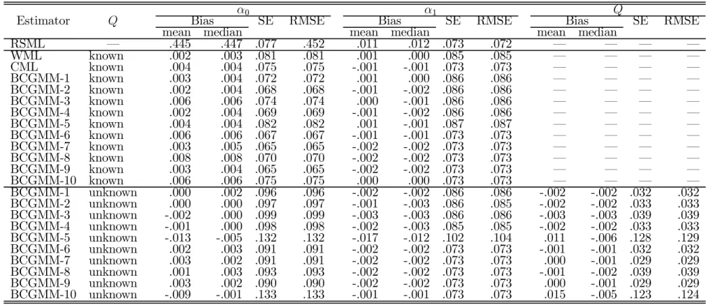
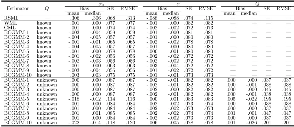
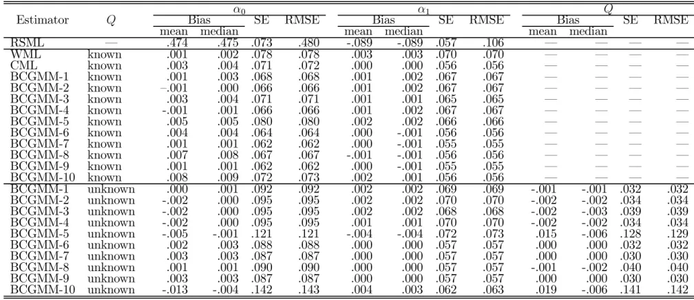
The results of the experiments are reported in Tables 3-6. In all cases, it is clear that the RSML estimator is upwardly biased. Even in design B, where only the pro-portion of the stratum 0 is different in the sample and in the population, its bias is above 30% for α0and almost 9% for α1. In contrast, all the bias-corrected estimators
display very small biases in all cases. However, their performance in terms of effi-ciency is not at all uniform. Indeed, according to this criterium, the estimators based on g2(θ) (BCGMM6-BCGMM10) are clearly superior to their counterparts based
on g1(θ)(BCGMM1-BCGMM5), particularly regarding the estimation of α1.
More-over, in each one of those two sets of estimators, those based on ge(Q) (BCGMM5
and BCGMM10) exhibited systematically higher variability in the estimation of α0.
When Q is known, the simpler WML and CML estimators seem to be as efficient as their extensions (BCGMM1-BCGMM5 and BCGMM6-BCGMM10, respectively)
when estimating α1. In effect, the extra moment conditions used by the BCGMM
estimators leads to sizable gains only in the precision of the estimator for α0.
Sim-ilarly, knowledge on Q appears to be important only for gaining precision in the estimation of the intercept.
Tables 3-6 about here
6.2
Probit model
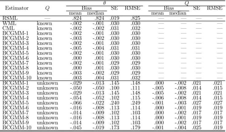
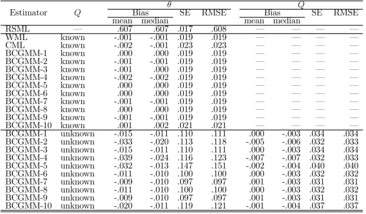
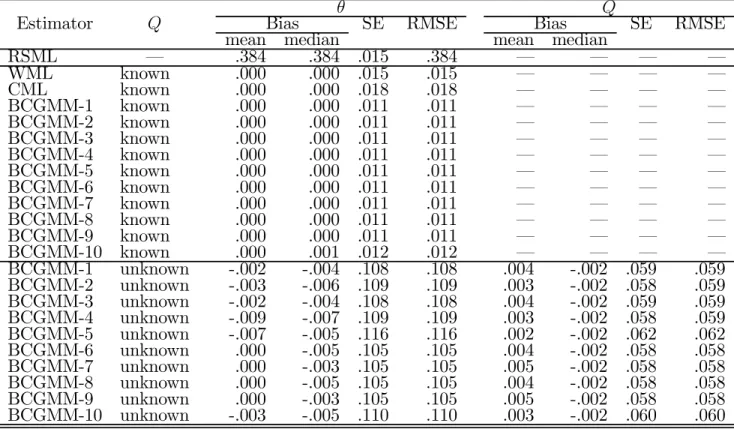
In this second simulation study we generated a pure CBS of binary data, consider-ing a Probit model, Pr (Y = 1|x, θ) = Φ (xθ), where x denotes a sconsider-ingle exogenous variable which was generated according to the normal distribution N (2, 0.5). Sev-eral values for the proportion of the stratum containing individuals choosing Y = 1 in the population, Q1 = Q, were examined: 0.05, 0.1, 0.2, and 0.3. To produce
those probabilities, the parameter θ was set equal to -1.01095, -0.71879, -0.44077, and -0.26682, respectively. Again, in all cases we generated a sampling design where H1 = H0 = H = 0.5.
Tables 7-10 present the results obtained for these experiments. The conclusions are very similar to those reported for the other design. Again, the RSML estimator is clearly upwardly biased in all experiments, displaying biases ranging from 81.5% to 88.1%, and all the bias-corrected estimators assuming Q known exhibit only small distortions in all cases. When Q is unknown, however, the BCGMM estimators display now some bias for higher levels of stratification, particularly those based on g1(θ) and ge(Q). Also in contrast to the previous design, the gain in precision that
results from knowledge on Q is now enormous, although the BCGMM estimators for Q are again approximately unbiased in all cases.
Tables 7-10 about here
7
Conclusion
In this paper we suggested several alternative BCGMM estimators to deal with ESS in parametric models. Their derivation was very simple and intuitive, presenting also
the advantages of giving rise to a bunch of moment-based estimators appropriate for both cases where the marginal strata probabilities are known and unknown and including most of the likelihood-based estimators existing in the literature as partic-ular cases. The results obtained in both the Monte Carlo experiments suggest that, in small samples, the best BCGMM estimators result from combining the Manski and McFadden (1981) bias-corrected moment indicators g2(θ) with any one of the
four alternative Manski and Lerman (1981)-type bias corrections for the equations defining the population strata probabilities, ga(Q), gb(Q), gc(Q) or gd(Q).
References
Artis, M.; Ayuso, M.; Guillén, M. Modelling Different Types of Automobile Insur-ance Fraud Behaviour in the Spanish Market. InsurInsur-ance: Mathematics and Economics 1999, 24, 67-81.
Cosslett, S. Efficient Estimation of Discrete-Choice Models. In Structural Analysis of Discrete Data with Econometric Applications; Manski, C., McFadden, D., Eds.; The MIT Press, 1981a; 51-111.
Cosslett, S. Maximum Likelihood Estimator for Choice-Based Samples. Economet-rica 1981b, 49 (5), 1289-1316.
Early, D.W. A Microeconomic Analysis of Homelessness: An Empirical Investiga-tion Using Choice-Based Sampling. Journal of Housing Economics 1999, 8 (4), 312-327.
Hansen, L.P. Large Sample Properties of Generalised Method of Moments Estima-tors. Econometrica 1982, 50(4), 1029-1054.
Imbens, G. An Efficient Method of Moments Estimator for Discrete Choice Models with Choice-Based Sampling, Econometrica 1992, 60 (5), 1187-1214.
Imbens, G.W.; Lancaster, T. Efficient Estimation and Stratified Sampling. Journal of Econometrics 1996, 74 (2), 289-318.
Kitamura, R.; Yamamoto, T.; Sakai, H. A Methodology for Weighting Observations from Complex Endogenous Sampling. Transportation Research Part B 2003, 37 (4), 387-401.
Manski, C.; Lerman, S. The Estimation of Choice Probabilities from Choice Based Samples. Econometrica 1977, 45 (8), 977-1988.
Manski, C.; McFadden, D. Alternative Estimators and Sample Designs for Discrete Choice Analysis. In Structural Analysis of Discrete Data with Econometric Applications; Manski, C., McFadden, D., Eds.; The MIT Press, 1981; 2-50.
Newey, W.K.; McFadden, D. Large Sample Estimation and Hypothesis Testing. In Handbook of Econometrics; Engle, R.F., McFadden, D.L., Eds.; Elsevier Science, 1994; Vol. 4, 2111-2245.
Newey, W. K.; Smith, R. J. Higher Order Properties of GMM and Generalized Empirical Likelihood Estimators. Econometrica 2004, 72 (1), 219-255.
8
Appendix
8.1
Derivation of the properties of the bias functions
The properties of the bias functions bs and bx presented in (7)-(10) are obtained as
follows: E¡b−1s ¢ = Z X X s∈S Z Ys b−1s bsf (y|x, θ) f (x) dydx = Z X X s∈S Z Ys f (y|x, θ) f (x) dydx = 1,
E¡b−1x ¢ = X s∈S Z Ys Z X b−1s bsf (y|x, θ) f (x) dydx = Z X b−1s f (x)X s∈S bsdx Z Ys f (y|x, θ) dy = Z X b−1s f (x) bsdx = 1, E · b−1s Z Yt f (y|x, θ) dy ¸ = Z X X s∈S Z Ys b−1s Z Yt f (y|x, θ) dybs(Q) f (y|x, θ) f (x) dydx = Z X Z Yt f (y|x, θ) f (x) dydxX s∈S Z Ys f (y|x, θ) dy = Z X Z Yt f (y|x, θ) f (x) dydx = Qt, E · b−1x Z Yt f (y|x, θ) dy ¸ = X s∈S Z Ys Z X b−1x Z Yt f (y|x, θ) dybz(θ, Q) f (y|x, θ) f (x) dydx = Z X b−1x Z Yt f (y|x, θ) dyX s∈S bs Z Ys f (y|x, θ) f (x) dydx = Z X b−1x Z Yt f (y|x, θ) bxf (x) dydx = Z X Z Yt f (y|x, θ) f (x) dydx = Qt, E · b−1s bx Z Yt f (y|x, θ) dy ¸ = Z X X s∈S Z Ys b−1s bx Z Yt f (y|x, θ) dybz(θ, Q) f (y|x, θ) f (x) dydx = Z X bx Z Yt f (y|x, θ) dyf (x) dxX s∈S Z Ys f (y|x, θ) dy = EX · bx Z Yt f (y|x, θ) dy ¸
and E¡b−1x ∇θbx ¢ = X s∈S Z Ys Z X b−1x X s∈S bs Z Ys ∇θf (y|x, θ) dybz(θ, Q) f (y|x, θ) f (x) dydx = Z X b−1x X s∈S bs Z Ys ∇θf (y|x, θ) dy X s∈S bs Z Ys f (y|x, θ) f (x) dydx = Z X b−1x X s∈S bs Z Ys ∇θf (y|x, θ) dybx(θ, Q) f (x) dx = Z X X s∈S bs Z Ys ∇θf (y|x, θ) dyf (x) dx = EX(∇θbx).
8.2
Moment indicators for the Monte Carlo simulation
The main components of the moment indicators that characterize each estimator may be specialized to the models simulated as described in Table 11.
Table 1: Alternative estimators and moment indicators Estimator g (β) g (θ)RS g1(θ) g2(θ) ga(Q) gb(Q) gc(Q) gd(Q) ge(Q) g (H) RSML × WML × CML × BCGMM1 × × × BCGMM2 × × × BCGMM3 × × × BCGMM4 × × × BCGMM5 × × × BCGMM6 × × × BCGMM7 × × × BCGMM8 × × × BCGMM9 × × × BCGMM10 × × ×
Table 2: Normal linear model Design X θ C Q
A N (0, 1) (0, 1, 1) 0.954 0.25 B N (0, 1) (0, 1, 1) 0 0.5 C E (1) − 1 (0, 1, 1) 0.802 0.25 D N (0, 1) (0, 0.5, 1) 0.954 0.194
Table 3: Normal linear model: Monte Carlo results for design A (5000 replications; N = 200)
α0 α1 Q
Estimator Q Bias SE RMSE Bias SE RMSE Bias SE RMSE
mean median mean median mean median
RSML – .445 .447 .077 .452 .011 .012 .073 .072 – – – – WML known .002 .003 .081 .081 .001 .000 .085 .085 – – – – CML known .004 .004 .075 .075 -.001 -.001 .073 .073 – – – – BCGMM-1 known .003 .004 .072 .072 .001 .000 .086 .086 – – – – BCGMM-2 known .002 .004 .068 .068 -.001 -.002 .086 .086 – – – – BCGMM-3 known .006 .006 .074 .074 .000 -.001 .086 .086 – – – – BCGMM-4 known .002 .004 .069 .069 -.001 -.002 .086 .086 – – – – BCGMM-5 known .004 .004 .082 .082 .001 -.001 .087 .087 – – – – BCGMM-6 known .006 .006 .067 .067 -.001 -.001 .073 .073 – – – – BCGMM-7 known .003 .005 .065 .065 -.002 -.002 .073 .073 – – – – BCGMM-8 known .008 .008 .070 .070 -.002 -.002 .073 .073 – – – – BCGMM-9 known .003 .004 .065 .065 -.002 -.002 .073 .073 – – – – BCGMM-10 known .006 .006 .075 .075 .000 .000 .073 .073 – – – – BCGMM-1 unknown .000 .002 .096 .096 -.002 -.002 .086 .086 -.002 -.002 .032 .032 BCGMM-2 unknown .000 .000 .097 .097 -.001 -.003 .086 .085 -.002 -.002 .033 .033 BCGMM-3 unknown -.002 .000 .099 .099 -.003 -.003 .086 .086 -.003 -.003 .039 .039 BCGMM-4 unknown -.001 .000 .098 .098 -.002 -.003 .085 .085 -.002 -.002 .033 .033 BCGMM-5 unknown -.013 -.005 .132 .132 -.017 -.012 .102 .104 .011 -.006 .128 .129 BCGMM-6 unknown .002 .003 .091 .091 -.002 -.002 .073 .073 -.001 -.001 .032 .032 BCGMM-7 unknown .003 .002 .091 .091 -.002 -.002 .073 .073 .000 -.001 .029 .029 BCGMM-8 unknown .001 .003 .093 .093 -.002 -.002 .073 .073 -.001 -.002 .039 .039 BCGMM-9 unknown .003 .002 .090 .090 -.002 -.002 .073 .073 .000 -.001 .029 .029 BCGMM-10 unknown -.009 -.001 .133 .133 -.001 -.001 .073 .073 .015 -.005 .123 .124
Table 4: Normal linear model: Monte Carlo results for design B (5000 replications; N = 200)
α0 α1 Q
Estimator Q Bias SE RMSE Bias SE RMSE Bias SE RMSE
mean median mean median mean median
RSML – .306 .306 .068 .313 -.088 -.088 .074 .115 – – – – WML known .001 .000 .077 .077 -.001 .000 .082 .082 – – – – CML known .001 .000 .074 .074 -.002 -.002 .072 .073 – – – – BCGMM-1 known -.003 -.004 .059 .059 -.001 .000 .081 .081 – – – – BCGMM-2 known -.004 -.005 .057 .057 -.001 .000 .080 .080 – – – – BCGMM-3 known -.001 -.001 .065 .065 -.002 -.002 .078 .078 – – – – BCGMM-4 known -.004 -.005 .057 .057 -.001 .000 .080 .080 – – – – BCGMM-5 known .001 .000 .078 .078 .000 .001 .080 .080 – – – – BCGMM-6 known -.001 -.002 .056 .056 -.002 -.002 .072 .072 – – – – BCGMM-7 known -.002 -.003 .056 .056 -.002 -.002 .072 .072 – – – – BCGMM-8 known .001 .000 .063 .063 -.003 -.004 .072 .072 – – – – BCGMM-9 known -.003 -.004 .056 .056 -.001 -.002 .072 .072 – – – – BCGMM-10 known .003 .003 .075 .075 -.001 -.001 .073 .073 – – – – BCGMM-1 unknown .000 .000 .087 .087 -.002 -.001 .082 .082 .000 .000 .037 .037 BCGMM-2 unknown .000 .000 .087 .087 -.002 -.001 .082 .082 .000 -.001 .038 .038 BCGMM-3 unknown .000 .000 .087 .087 -.002 .000 .082 .082 .000 .000 .045 .045 BCGMM-4 unknown .000 .000 .087 .087 -.002 -.001 .082 .082 .000 -.001 .038 .038 BCGMM-5 unknown -.018 -.012 .114 .116 .000 .001 .083 .083 .005 -.022 .195 .195 BCGMM-6 unknown .001 .000 .084 .084 -.002 -.002 .073 .074 .000 .000 .038 .038 BCGMM-7 unknown .001 .000 .084 .084 -.002 -.002 .073 .073 .000 .000 .037 .037 BCGMM-8 unknown .001 .001 .085 .085 -.002 -.002 .074 .074 .001 .001 .047 .047 BCGMM-9 unknown .001 .000 .084 .084 -.002 -.002 .073 .073 .000 .000 .037 .037 BCGMM-10 unknown -.022 -.014 .118 .120 .006 .005 .078 .078 .001 -.026 .201 .201
Table 5: Normal linear model: Monte Carlo results for design C (5000 replications; N = 200)
α0 α1 Q
Estimator Q Bias SE RMSE Bias SE RMSE Bias SE RMSE
mean median mean median mean median
RSML – .474 .475 .073 .480 -.089 -.089 .057 .106 – – – – WML known .001 .002 .078 .078 .003 .003 .070 .070 – – – – CML known .003 .004 .071 .072 .000 .000 .056 .056 – – – – BCGMM-1 known .001 .003 .068 .068 .001 .002 .067 .067 – – – – BCGMM-2 known —.001 .000 .066 .066 .001 .002 .067 .067 – – – – BCGMM-3 known .003 .004 .071 .071 .001 .001 .065 .065 – – – – BCGMM-4 known -.001 .001 .066 .066 .001 .002 .067 .067 – – – – BCGMM-5 known .005 .005 .080 .080 .002 .002 .066 .066 – – – – BCGMM-6 known .004 .004 .064 .064 .000 -.001 .056 .056 – – – – BCGMM-7 known .001 .001 .062 .062 .000 -.001 .055 .055 – – – – BCGMM-8 known .007 .008 .067 .067 -.001 -.001 .056 .056 – – – – BCGMM-9 known .001 .001 .062 .062 .000 -.001 .055 .055 – – – – BCGMM-10 known .008 .009 .072 .073 .002 .001 .056 .056 – – – – BCGMM-1 unknown .000 .001 .092 .092 .002 .002 .069 .069 -.001 -.001 .032 .032 BCGMM-2 unknown -.002 .000 .095 .095 .002 .002 .070 .070 -.002 -.002 .034 .034 BCGMM-3 unknown -.002 .000 .095 .095 .002 .002 .068 .068 -.002 -.003 .039 .039 BCGMM-4 unknown -.002 .000 .095 .095 .001 .001 .070 .070 -.002 -.002 .034 .034 BCGMM-5 unknown -.005 -.001 .121 .121 -.004 -.004 .072 .073 .015 -.006 .128 .129 BCGMM-6 unknown .002 .003 .088 .088 .000 .000 .057 .057 .000 .000 .032 .032 BCGMM-7 unknown .003 .003 .087 .087 .000 .000 .057 .057 .000 .000 .030 .030 BCGMM-8 unknown .001 .001 .090 .090 .000 .000 .057 .057 -.001 -.002 .040 .040 BCGMM-9 unknown .003 .003 .087 .087 .000 .000 .057 .057 .000 .000 .030 .030 BCGMM-10 unknown -.013 -.004 .142 .143 .004 .003 .062 .063 .019 -.006 .141 .142
Table 6: Normal linear model: Monte Carlo results for design D (5000 replications; N = 200)
α0 α1 Q
Estimator Q Bias SE RMSE Bias SE RMSE Bias SE RMSE
mean median mean median mean median
RSML – .619 .620 .067 .623 .041 .040 .072 .083 – – – – WML known .002 .002 .076 .076 .001 .001 .084 .084 – – – – CML known .002 .001 .068 .068 .001 .000 .069 .069 – – – – BCGMM-1 known -.006 -.003 .063 .064 .001 .000 .085 .085 – – – – BCGMM-2 known -.007 -.005 .062 .062 .000 -.001 .085 .085 – – – – BCGMM-3 known -.002 .000 .064 .064 .001 -.001 .085 .085 – – – – BCGMM-4 known -.007 -.005 .062 .062 -.001 -.001 .085 .085 – – – – BCGMM-5 known .003 .005 .078 .078 -.002 -.002 .088 .088 – – – – BCGMM-6 known -.004 -.004 .056 .056 .000 -.001 .070 .070 – – – – BCGMM-7 known -.006 -.005 .055 .055 -.001 -.001 .070 .070 – – – – BCGMM-8 known .000 .000 .060 .060 -.001 -.002 .070 .070 – – – – BCGMM-9 known -.006 -.006 .055 .055 -.001 -.001 .070 .070 – – – – BCGMM-10 known .001 .000 .067 .067 -.005 -.005 .072 .072 – – – – BCGMM-1 unknown .002 .004 .100 .100 .000 -.002 .086 .086 .002 .002 .030 .030 BCGMM-2 unknown .001 .004 .101 .101 .000 -.001 .084 .084 .001 .002 .031 .031 BCGMM-3 unknown -.001 .002 .106 .106 -.001 -.002 .086 .086 .001 .001 .036 .036 BCGMM-4 unknown .001 .004 .101 .101 .000 -.001 .084 .084 .001 .002 .031 .031 BCGMM-5 unknown -.005 .001 .137 .137 -.011 -.008 .097 .098 .012 .001 .094 .095 BCGMM-6 unknown .005 .004 .093 .094 .000 .000 .070 .070 .003 .003 .027 .027 BCGMM-7 unknown .006 .005 .093 .093 .000 .000 .070 .070 .004 .003 .025 .026 BCGMM-8 unknown .004 .004 .096 .096 .000 -.001 .070 .070 .003 .003 .032 .032 BCGMM-9 unknown .006 .005 .092 .093 .000 .000 .070 .070 .004 .003 .025 .026 BCGMM-10 unknown -.004 .002 .143 .143 .000 -.002 .070 .070 .013 .002 .086 .087
Table 7: Probit model: Monte Carlo results for Q = 0.05 (5000 replications; N = 200)
θ Q
Estimator Q Bias SE RMSE Bias SE RMSE
mean median mean median
RSML – .824 .824 .019 .825 – – – – WML known -.002 -.001 .030 .030 – – – – CML known -.002 -.002 .031 .032 – – – – BCGMM-1 known -.002 -.001 .030 .030 – – – – BCGMM-2 known -.003 -.002 .030 .030 – – – – BCGMM-3 known -.002 -.001 .030 .030 – – – – BCGMM-4 known -.005 -.004 .031 .031 – – – – BCGMM-5 known -.002 -.001 .030 .030 – – – – BCGMM-6 known .000 .001 .030 .030 – – – – BCGMM-7 known -.002 -.001 .029 .029 – – – – BCGMM-8 known .000 .001 .030 .030 – – – – BCGMM-9 known -.003 -.002 .029 .029 – – – – BCGMM-10 known .003 .004 .031 .032 – – – – BCGMM-1 unknown -.029 -.013 .145 .148 .000 -.002 .021 .021 BCGMM-2 unknown -.050 -.050 .100 .111 -.005 -.008 .014 .015 BCGMM-3 unknown -.029 -.013 .145 .148 -.005 -.002 .021 .021 BCGMM-4 unknown -.054 -.052 .102 .115 -.006 -.008 .014 .015 BCGMM-5 unknown -.066 -.022 .240 .249 -.001 -.003 .027 .027 BCGMM-6 unknown -.016 -.008 .113 .114 .000 -.001 .019 .019 BCGMM-7 unknown -.014 -.009 .102 .103 .000 -.002 .017 .017 BCGMM-8 unknown -.016 -.008 .113 .114 .000 -.001 .019 .019 BCGMM-9 unknown -.014 -.009 .102 .103 .000 -.002 .017 .017 BCGMM-10 unknown -.045 -.019 .173 .179 -.001 -.004 .025 .019
Table 8: Probit model: Monte Carlo results for Q = 0.1 (5000 replications; N = 200)
θ Q
Estimator Q Bias SE RMSE Bias SE RMSE
mean median mean median
RSML – .607 .607 .017 .608 – – – – WML known -.001 -.001 .019 .019 – – – – CML known -.002 -.001 .023 .023 – – – – BCGMM-1 known .000 .000 .019 .019 – – – – BCGMM-2 known -.001 -.001 .019 .019 – – – – BCGMM-3 known -.001 .000 .019 .019 – – – – BCGMM-4 known -.002 -.002 .019 .019 – – – – BCGMM-5 known .000 .000 .019 .019 – – – – BCGMM-6 known .000 .000 .019 .019 – – – – BCGMM-7 known -.001 -.001 .019 .019 – – – – BCGMM-8 known .000 .000 .019 .019 – – – – BCGMM-9 known -.001 -.001 .019 .019 – – – – BCGMM-10 known .001 .002 .021 .021 – – – – BCGMM-1 unknown -.015 -.011 .110 .111 .000 -.003 .034 .034 BCGMM-2 unknown -.033 -.020 .113 .118 -.005 -.006 .032 .033 BCGMM-3 unknown -.015 -.011 .110 .111 .000 -.003 .034 .034 BCGMM-4 unknown -.039 -.024 .116 .123 -.007 -.007 .032 .033 BCGMM-5 unknown -.032 -.013 .147 .151 -.002 -.004 .040 .040 BCGMM-6 unknown -.011 -.010 .100 .100 .000 -.003 .032 .032 BCGMM-7 unknown -.009 -.010 .097 .097 .001 -.003 .031 .031 BCGMM-8 unknown -.011 -.010 .100 .100 .000 -.003 .032 .032 BCGMM-9 unknown -.009 -.010 .097 .097 .001 -.003 .031 .031 BCGMM-10 unknown -.020 -.011 .119 .121 -.001 -.004 .037 .037
Table 9: Probit model: Monte Carlo results for Q = 0.2 (5000 replications; N = 200)
θ Q
Estimator Q Bias SE RMSE Bias SE RMSE
mean median mean median
RSML – .384 .384 .015 .384 – – – – WML known .000 .000 .015 .015 – – – – CML known .000 .000 .018 .018 – – – – BCGMM-1 known .000 .000 .011 .011 – – – – BCGMM-2 known .000 .000 .011 .011 – – – – BCGMM-3 known .000 .000 .011 .011 – – – – BCGMM-4 known .000 .000 .011 .011 – – – – BCGMM-5 known .000 .000 .011 .011 – – – – BCGMM-6 known .000 .000 .011 .011 – – – – BCGMM-7 known .000 .000 .011 .011 – – – – BCGMM-8 known .000 .000 .011 .011 – – – – BCGMM-9 known .000 .000 .011 .011 – – – – BCGMM-10 known .000 .001 .012 .012 – – – – BCGMM-1 unknown -.002 -.004 .108 .108 .004 -.002 .059 .059 BCGMM-2 unknown -.003 -.006 .109 .109 .003 -.002 .058 .059 BCGMM-3 unknown -.002 -.004 .108 .108 .004 -.002 .059 .059 BCGMM-4 unknown -.009 -.007 .109 .109 .003 -.002 .058 .059 BCGMM-5 unknown -.007 -.005 .116 .116 .002 -.002 .062 .062 BCGMM-6 unknown .000 -.005 .105 .105 .004 -.002 .058 .058 BCGMM-7 unknown .000 -.003 .105 .105 .005 -.002 .058 .058 BCGMM-8 unknown .000 -.005 .105 .105 .004 -.002 .058 .058 BCGMM-9 unknown .000 -.003 .105 .105 .005 -.002 .058 .058 BCGMM-10 unknown -.003 -.005 .110 .110 .003 -.002 .060 .060
Table 10: Probit model: Monte Carlo results for Q = 0.3 (5000 replications; N = 200)
θ Q
Estimator Q Bias SE RMSE Bias SE RMSE
mean median mean median
RSML – .235 .235 .014 .235 – – – – WML known .000 .000 .014 .014 – – – – CML known -.001 .000 .016 .016 – – – – BCGMM-1 known .000 .000 .007 .007 – – – – BCGMM-2 known .000 .000 .007 .007 – – – – BCGMM-3 known .000 .000 .007 .007 – – – – BCGMM-4 known .000 .000 .007 .007 – – – – BCGMM-5 known -.001 .000 .008 .008 – – – – BCGMM-6 known .000 .000 .007 .007 – – – – BCGMM-7 known .000 .000 .007 .007 – – – – BCGMM-8 known .000 .000 .007 .007 – – – – BCGMM-9 known .000 .000 .007 .007 – – – – BCGMM-10 known -.001 .000 .008 .008 – – – – BCGMM-1 unknown -.002 -.003 .117 .117 .003 -.001 .079 .079 BCGMM-2 unknown -.002 -.003 .117 .117 .003 -.002 .079 .079 BCGMM-3 unknown -.002 -.003 .117 .117 .003 -.001 .079 .079 BCGMM-4 unknown -.003 -.003 .117 .117 .002 -.002 .079 .079 BCGMM-5 unknown .007 .004 .113 .114 .010 .003 .081 .081 BCGMM-6 unknown -.002 -.003 .116 .116 .003 -.002 .079 .079 BCGMM-7 unknown -.002 -.004 .115 .115 .003 -.003 .079 .079 BCGMM-8 unknown -.002 -.003 .116 .116 .003 -.002 .079 .079 BCGMM-9 unknown -.002 -.004 .115 .115 .003 -.003 .079 .079 BCGMM-10 unknown .012 .006 .111 .112 .013 .004 .081 .082
Table 11: Moment indicators for the Monte Carlo study
.
Normal linear model Binary model
g (θ)RS x0 y−x0α σ2 1 2σ2 ·³ y−x0α σ ´2 − 1 ¸ x∇θPr(Y =1|x,θ)[y−Pr(Y =1|x,θ)] Pr(Y =1|x,θ)[1−Pr(Y =1|x,θ)] g (Q)RS Q− Φ¡−C+xσ 0α¢ Q− Pr (Y = 1|x, θ) g (H) H− 1 (s = 1) H− y bs (1− H) 1 (y < C) + Q(1−H)+HQ 1 (y ≥ C) 1−H1−Q + y ³ H Q − 1−H1−Q ´ bx 1− H + HQΦ ¡−C+x0α σ ¢ 1−H 1−Q + Pr (Y = 1|x, θ) ³ H Q − 1−H 1−Q ´ ∇θbx x0 σ H Qφ ¡−C+x0α σ ¢ −−C+x2σ30α H Qφ ¡−C+x0α σ ¢ x∇θPr (Y = 1|x, θ) ³ H Q − 1−H1−Q ´