()* + * ,!-)( ./ *0 ( * 10%+( *0)(* + /(+(2.3
) 4.5 (5 -4(* ( ,!*(,,()
Physics Department, Faculty of Science, Alexandria University, 21511 Alexandria, Egypt *Corresponding Author: ms241178@hotmail.com
Abstract
The full energy peak efficiency of HPGe detector is computed using a new analytical approach. The approach explains the effect of self.attenuation of the source matrix, the attenuation by the source container and the detector housing materials on the detector efficiency. The experimental calibration process was done using radioactive spherical sources containing aqueous 152Eu radionuclide which produces photons with a wide range of energies from 121 up to 1408 keV. The comparison shows a good agreement between the measured and calculated efficiencies for the detector using spherical sources.
Keywords: HPGe detectors, Spherical sources, Full.energy peak efficiency, Self.attenuation.
1. Introduction
Nomenclatures
AS Radionuclide activity, Bq
Ci Correction factors due to dead time and radionuclide decay
Cd The decay correction for the calibration source from the reference time to the run time
d (θ,φ) Possible path length travelled by the photon within the detector active volume, m
d Average path length travelled by a photon through the detector, m
fatt Attenuation factor of the detector dead layer and end cap material
fcap Attenuation factor of the detector end cap material
flay Attenuation factor of the detector dead layer
ho Distance between the source active volume and the detector upper surface, m
k Distance between the detector end cap and the detector upper surface, m
L Detector length, m
N(E) Number of counts in the full.energy peak which can be obtained using Genie 2000 software
P(E) Photon emission probability at energy E R Detector radius , m
Ra Inner radius of the detector end cap, m
S Source radius, m
Ssc Attenuation factor of the source container material
Sself Self.attenuation factor of the source matrix
T Measuring time, s
ta Upper surface thickness of the end cap, m
tDF Upper surface thickness of the dead layer, m
tDS Side surface thickness of the dead layer, m
tw Side surface thickness of the end cap, m ( , )
t′θ ϕ Possible path length travelled by the photon within the detector dead layer ,m
1
t′ photon path length through the upper surface of the dead layer, m ( , )
t′′θ ϕ Possible path length travelled by the photon within the detector end cap material, m
1
t′′ Photon path length through the upper surface of the detector end cap material, m
2
t′ photon path length through the side surface of the dead layer, m 2
t′′ Photon path length through the side surface of the detector end cap material, m
t Average path length travelled by a photon inside the spherical source, m
Greek Symbols
α Angle between the lateral distance ρ and the detector’s major axis, deg.
$T Interval between the source activity reference time and the measurement time, s
x The source container thickness, m
1 Percentage deviations between the calculated with Sself and the
measured full.energy peak efficiency values, %
2 Percentage deviations between the calculated without Sself and the
Measured full.energy peak efficiency values, %
lay
δ Average path length travelled by a photon through the detector dead layer, m
cap
δ Average path length traveled by a photon through the detector end cap material, m
self S cal−with
ε Calculated with self.attenuation factor self
S cal−without
ε Calculated with / without self.attenuation factor
εg Geometrical efficiency
εi Intrinsic efficiency
εmeas Experimentally measured efficiencies
εpoint Detector efficiency with respect to point source
εsph Detector efficiency with respect to spherical source
θ Polar angle, deg.
λ Decay constant ,s.1
Attenuation coefficient of the detector material, m.1
*c Attenuation coefficient of the source container material, m
.1
cap Attenuation coefficients of the detector end cap material, m
.1
lay Attenuation coefficients of the detector dead layer, m
.1
*s Attenuation coefficient of the source matrix, m.1
ρ Lateral distance, m
ρʹ Maximum integration limit, m
σε The uncertainty in the full.energy peak efficiency
φ Azimuthal angle, deg. Solid angle
these analytical expressions into a numerical integration computer program. Moreover, they introduced a new theoretical approach [13.16] based on that Direct Statistical method to determine the detector efficiency for an isotropic radiating point source at any arbitrary position from a cylindrical detector, as well as the extension of this approach to volume sources.
first is the accurate analytical calculation of the average path length covered by the photon in each of the following: the detector active volume, the source matrix, the source container, the dead layer and the end cap of the detector, second is the geometrical solid angle G.
2. Mathematical Viewpoint
2.1. The Case of a Non Axial Point Source
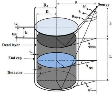
Consider a right circular cylindrical (2R×L), detector and an arbitrarily positioned isotropic radiating point source located at a distance h from the detector top surface, and at a lateral distance ρ from its axis. The efficiency of the detector with respect to point source is given as follows [14]:
i g att
po f ε ε
ε int= (1) where εi and εg are the intrinsic and the geometrical efficiencies which are
derived by Abbas et al. [14]. fatt is the attenuation factor of the detector dead layer
and end cap material, the air attenuation is neglected. In section 2.1.2, this factor will be recalculated by a new method which is dependent on calculating the average path length within these materials.
2.1.1. Intrinsic and geometrical efficiencies
The intrinsic, εi, and geometrical, εg, efficiencies are represented by Eqs. (2) and (3) respectively
d
i e
ε = − −
1 (2)
π ε
4
=
g (3) where * is the attenuation coefficient of the detector material and depends on the energy, while d is the average path length travelled by a photon through the detector, G is the solid angle subtended by the source.detector and they are represented by Eqs. (4) and (5) respectively. These will be discussed in details according to the source detector configuration as shown below.
( )
∫ ∫( )
= ∫
∫
= ϕ θ
ϕ θ θ ϕ θ ϕ
θ d d d
dd d d d
sin , ,
(4)
where θ and φ arethe polar and the azimuthal anglesrespectively, d(θ,φ) is the possible path length travelled by the photon within the detector active volume.
∫ ∫ =
ϕ θ
ϕ θ θd d
sin (5)
lateral displacement of the source is smaller than or equal the detector circular face’s radius (ρ ≤ R) and (ii) the lateral distance of the source is greater than the detector circular face’s radius (ρ > R). The two cases have been treated by Abbas et al. [14]. The values of the polar and the azimuthal angles based on the source to detector configuration are shown in Table 1.
Table 1. Values of Polar and Azimuthal Angles Based on the Source to Detector Configuration [13].
The polar angles The azimuthal angles
1 1 1 2 1 3 1 4
t a n
ta n
t a n
ta n R h L R h R h L R h ρ θ ρ θ ρ θ ρ θ − − − − − = + − = + = + + = 2 2 1 2 2 1 tan tan c c R h L R h ρ θ ρ θ − − − = + − ′= ( ) 2 2 1 max max
tan ( )
T
R h h L
ρ
θ= − − ϕ =ϕ′
+
2 2 2 2
2 2 2 2
max 1 max 1 tan 2 tan
( ) tan 2 ( ) tan
cos
cos
R h
h
R h L
h L ρ θ ϕ ρ θ ρ θ ϕ ρ θ − − − + = − + + ′ = + 1 s in c R ϕ ρ − =
2.1.2. Attenuation factor ( fatt)
The attenuation factor fatt is expressed as:
fatt = flay + fcap (6) where flay and fcap are the attenuation factors of the detector dead layer and end cap material respectively and they are given by:
lay lay e flay δ −
= , cap cap
e fcap
δ −
= (7)
where lay and cap are the attenuation coefficients of the detector dead layer and end cap material respectively, while δlayand δcap are the average path length
travelled by a photon through the detector dead layer and end cap material respectively and they are represented as follow:
where t′( )θ,ϕ and t′′( )θ,ϕ are the possible path lengths travelled by the photon
within the detector dead layer and end cap material respectively.
Let us consider the detector having a dead layer which covers its upper surface with thickness tDF and its side surface with thickness tDS, as shown in Fig. 1. The possible path lengths and the average path length travelled by the photon within the dead layer for cases (ρ≤R) and (ρ>R) are shown in Table 2, where t1′and t2′
represents the photon path length through the upper and the side surface of the dead layer respectively.
Consider the thickness of upper and side surface of the detector end cap material is ta and tw respectively, as shown in Fig. 1. The possible path lengths and the average path length travelled by the photon within the detector end cap material for cases (ρ≤R) and (ρ>R) are shown in Table 3, where t1′′ and t2′′ represents the photon path length through the upper and the side surface of the detector end cap material respectively. From Table 3 we observe that, the case in which (ρ > R) has two sub cases which are (R < ρ ≤ Ra) and (ρ > Ra), where Rais the inner radius of the detector end cap. There is a very important polar angle (θcap) which must be considered when we study the case in which (ρ > Ra) and this is given by:
− −
= −
k h
Ra cap
ρ
θ tan 1 (9)
where k is the distance between the detector end cap and the detector upper surface.
Table 2. The Possible Path Lengths and the Average Path Length Travelled by the Photon within the Dead Layer for Cases ρ ≤ R and ρ > R.
Table 3. Possible Path Lengths and the Average Path Length Travelled by the Photon within the Detector End Cap Material for Cases ρ ≤ R and ρ > R.
ρ ≤ R ρ > R
1 c o s
D F
t t
θ
′ = 1
c o s
D F t t θ ′ = ( ) ( )
2 2 2
2
2 2 2
2 2 2
c o s sin
s in
c o s s in
s in
1 s in
2 s in D S D S R t t R t R
ρ ϕ ρ ϕ
θ
ρ ϕ ρ ϕ
θ ρ ϕ θ + + − ′ = + − − + ≅ 1 2
l a y
Z I
δ = 3
4
l a y
Z I
δ =
2
m a x 4 2
1 1
0 0
1 0
s i n
s i n
Z t d d
t d d
θ π
ϕ θ θ
θ θ ϕ
θ θ ϕ
′ = ′ + ∫ ∫ ∫ ∫
m ax m ax
2
1 2
m a x 4
3 2 1
0 0
1 1
0 0
sin s in
s in sin
c
c c
c c
Z t d d t d d
t d d t d d
ϕ θ ϕ
θ
θ θ
θ ϕ θϕ
θ θ
θ ϕ θ θ ϕ θ
θ ϕ θ θ ϕ θ
′ ′ ′ ′ ′ ′ = + ′ ′ + + ∫ ∫ ∫ ∫ ∫ ∫ ∫ ∫
m a x 2
1
m a x 4 2
3 2 2
0 0
1 1
0 0
s i n s i n
s i n s i n
c c
c c c
c
Z t d d t d d
t d d t d d
θ ϕ θ ϕ
θ θ
θ ϕ θ ϕ
θ θ
θ ϕ θ θ ϕ θ
θ ϕ θ θ ϕ θ
′ ′ ′ ′ ′ = + ′ ′ + + ∫ ∫ ∫ ∫ ∫ ∫ ∫ ∫
(θ2 ≥ θ′c)
(θ2 < θ′c)
ρ ≤ R ρ > R
R < ρ ≤ Ra ρ > Ra
1
c o s
a
t t
θ
′′ = 1
c o s
a t t θ ′′ = 1 c o s
a t t θ ′′ = ( ) ( )
2 2 2
2
2 2
2 2 2 2
cos sin
sin
1 sin
cos sin 2
sin sin a w w a a R t t t R R
ρ ϕ ρ ϕ
θ
ρ ϕ
ρ ϕ ρ ϕ
θ θ + + − ′′ = + + − − ≅ 1 2
c a p
Z I
δ = ′ 3
4
c a p
Z I
δ = ′ 3
4
c a p
Z I
δ = ′
2 max 4 2 1 1 0 0 1 0 sin sin
Z t d d
t d d
θ π
ϕ θ
θ
θ θ ϕ
θ θ ϕ ′= ′′ ′′ + ∫ ∫ ∫ ∫ max 1 max 4 3 1 0 1 0 1 0 sin sin sin c c c c c
Z t d d
t d d
t d d
θ ϕ θ θ ϕ θ ϕ θ θ
θ ϕ θ
θ ϕ θ
θ ϕ θ
′ ′ ′ ′= ′′ ′′ + ′′ + ∫ ∫ ∫ ∫ ∫ ∫
m a x 1
m a x 4
3 1 1
0 0
1 0
sin sin
s in
c c c
c
c
Z t d d t d d
t d d
θ ϕ θ ϕ
θ θ
ϕ θ θ
θ ϕ θ θ ϕ θ
θ ϕ θ
′ ′ ′ ′= ′′ + ′′ ′′ + ∫ ∫ ∫ ∫ ∫ ∫
θ1 ≥ θcap
max m ax
1
m ax 4
3 2 1
0 0 1 1 0 0 sin sin sin sin cap c cap c c c c
Z t d d t d d
t d d t d d
θ ϕ θ ϕ
θ θ
θ ϕ θϕ
θ θ
θ ϕ θ θ ϕ θ
θ ϕ θ θ ϕ θ
′ ′ ′ ′ ′= ′′ + ′′ ′′ ′′ + + ∫ ∫ ∫ ∫ ∫ ∫ ∫ ∫
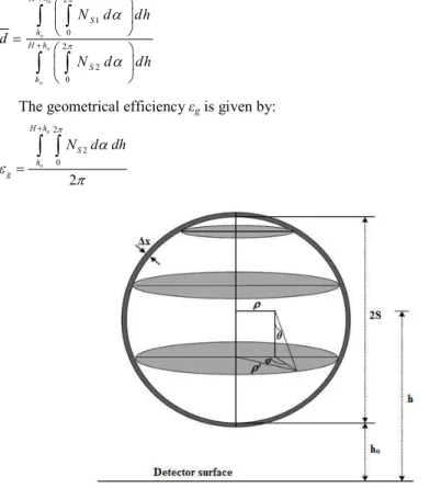
2.2. The case of a spherical source
The efficiency of a detector using spherical source has been treated before by Pibida et al. [15], but they deal with the case where the diameter of the source is smaller than that of the detector. In this work, we deal with the two cases, where the source diameter is smaller or bigger than the detector diameter and include a new treatment for the calculations.
The efficiency of a cylindrical detector with radius R and height L, arising from a spherical source with radius S, as shown in Fig. 2, is given by:
self sc att i g
sph
S S f
V
ε ε
ε
= (10)where V is the volume of the spherical source, V=34πS3. Sself is the self.
attenuation factor of the source matrix and Ssc is the attenuation factor of the source container material. The intrinsic and geometrical efficiencies are defined before in Eqs. (2) and (3) respectively, but the average path length d travelled by the photon through the detector and the solid angle will have new forms due to the geometry of Fig. 2. The average path length is expressed as:
2 1 0 2
2 0
o
o
o
o
H h
S h
H h
S h
N d dh d
N d dh π
π
α
α
+
+
=
∫ ∫
∫ ∫
(11)
The geometrical efficiency εg is given by:
2 2 0
2
o
o H h
S h g
N d dh π
α ε
π
+
=
∫ ∫
(12)where, 1 0 1 1 3 0 ( ) ( ) S R R
I d R
N
I d I d R
ρ
ρ
ρ ρ ρ
ρ ρ ρ ρ ρ
′ ′ ′ ≤ =
+ ′>
∫
∫
∫
(13) 2 0 2 2 4 0 ( ) ( ) S R RI d R
N
I d I d R
ρ
ρ
ρ ρ ρ
ρ ρ ρ ρ ρ
′ ′ ′ ≤ =
+ ′>
∫
∫
∫
(14)
where I1 and I2 are the numerator and the denominator of d equation obtained
by Abbas et al. [14] for the non.axial point source, α is the angle between the lateral distance ρ and the detector’s major axis, while ρʹ is the maximum integration limit and is given by [17]:
(h ho)(2S h ho)
ρ
′ = − − + (15)where hois the distance between the source active volume and the detector upper surface. The new forms of the average path length travelled by the photon through the detector dead layer and the detector end cap material are given by Eqs. (16) and (17) respectively.
2 3 0 2 2 0 o o o o H h S h
lay H h
S h
N d dh
N d dh π π α δ α + + =
∫ ∫
∫ ∫
(16) 2 4 0 2 2 0 o o o o H h S hcap H h
S h
N d dh
N d dh π π α δ α + + =
∫ ∫
∫ ∫
(17) where 1 0 3 1 3 0 ( ) ( ) S R RZ d R
N
Z d Z d R
ρ
ρ
ρ ρ ρ
ρ ρ ρ ρ ρ
′ ′ ′ ≤ =
+ ′>
∫
∫
∫
(18)
where Z1 and Z3 are as identified before in Table 2.
1 0 4 1 3 0 ( ) ( ) S R R
Z d R
N
Z d Z d R
ρ
ρ
ρ ρ ρ
ρ ρ ρ ρ ρ
′ ′ ′ ′ ≤ =
′ + ′ ′>
∫
∫
∫
where Z1′ and Z3′ are as identified before in Table 3.
For the spherical source, there is only one path length for the photon to exit from the source and is given by [17]:
2 2 2
s
d =U+ U +ρ′ −ρ (20) where
( o ) cos sin cos
U= h h− −S
θ ρ
+θ
ϕ
(21) The self.attenuation factor of the source matrix is given by:t self e S
S = − (22) where *s is the attenuation coefficient of the source matrix and the average path length ttravelled by a photon inside the spherical source is given by:
0
0
2 1 0 2
2 0
o
o H h
s h H h
s h
M d dh t
N d dh π
π
α
α
+
+
=
∫ ∫
∫ ∫
(23)
where,
1 0 1
1 2
0
( )
( )
s
s R
s s
R
g d R
M
g d g d R
ρ
ρ
ρ ρ ρ
ρ ρ ρ ρ ρ
′
′
′ ≤
=
+ ′>
∫
∫
∫
(24)
with
max
2 4
2
1
0 0 0
sin sin
s s s
g d d d d d d
ϕ
θ π θ
θ
θ ϕ θ
θ ϕ θ
=
∫ ∫
+∫ ∫
(25)max 4 max
1
2
0 0
sin sin sin
c c c
c c
s s s s
o
g d d d d d d d d d
θ ϕ θ ϕ θϕ
θ θ θ
θ ϕ θ
θ ϕ θ
θ ϕ θ
′ ′
′
=
∫ ∫
+∫ ∫
+∫ ∫
(26)If x is the source container thickness, the photon path length travelled through the source container is given by:
2 2 2 2 2 2
1
s
d′= U +
ρ
′ −ρ
− U +ρ
′ −ρ
(27) where U and ρʹ are defined before in Eqs. (21) and (15) respectively, while ρ′1is given by:
1 (h ho x)(2S h ho x)
ρ
′ = − + − + + (28)The attenuation factor of the container material is given by:
c ct
SC e
where *c is the attenuation coefficient of the source container material and the average path length travelled by a photon inside the source container is given by following equation:
0
0
2 1 0 2
2 0
o
o H h
s h
c H h
s h
M d dh t
N d dh π
π
α
α
+
+
′
=
∫ ∫
∫ ∫
(30)
where
1 0 1
1 2
0
( )
( )
s
s R
s s
R
g d R
M
g d g d R
ρ
ρ
ρ ρ
ρ ρ ρ
′
′
′ ′ ≤
′ =
′ + ′ ′>
∫
∫
∫
(31)
With:
max
2 4
2
1
0 0 0
sin sin
s s s
g d d d d d d
ϕ
θ π θ
θ
θ ϕ θ θ ϕ θ
′ =
∫ ∫
′ +∫ ∫
′ (32)max 4 max
1
2
0 0
sin sin sin
c c c
c c
s s s s
o
g d d d d d d d d d
θ ϕ θ ϕ θ ϕ
θ θ θ
θ ϕ θ θ ϕ θ θ ϕ θ
′ ′
′
′ =
∫ ∫
′ +∫ ∫
′ +∫ ∫
′ (33)3. Experimental setup
The full.energy peak efficiency was measured for a p.type Canberra HPGe cylindrical detector (Model GC1520) with relative efficiency 15 % (energy range from 50 keV to 10 MeV). Schematic from the manufacturer is illustrated in Fig. 3 and Table 4 lists its specifications. The spherical sources are made from rubber with volume 113 mL (with inner diameter 6 cm and wall thickness 0.16 cm) and 179.5 mL (with inner diameter 7 cm and wall thickness 0.22 cm) filled with an aqueous solution containing 152Eu radionuclide which emits γ.rays in the energy range from 121 keV to 1408 keV. The efficiency measurements were generated by positioning the sources over the end cap of the detector. In order to prevent dead time, the activity of the sources was kept low (5048 ± 50 Bq).
All sources were measured on the detector entrance window as an absorber to avoid the effect of β. and x.rays, so no correction was made for x.gamma coincidences. Since in most cases the accompanying x.ray were soft enough to be absorbed completely before entering the detector and also the angular correlation effects can be negligible for the low source.to.detector distance. It must be noted that gamma.gamma coincidences were not taken into account, what can induce deviations of the peaks area. In order to prevent dead time and pile up effects, the activity of the sources was kept lower than some kBq for the radionuclide in order to avoid high count rates when measuring at low distance, which implicates however long counting time at high distance.
energy tails appropriate for germanium detector. The spectra acquired by the gamma analyser software were analysed with the program using its automatic peak search and peak area calculations, along with changes in the peak fit using the interactive peak fit interface when necessary to reduce the residuals and error in the peak area values. The peak areas, live time, real time and starting time for each spectrum were entered in the spreadsheets that were used to perform the calculations necessary to generate the efficiency curves.
Fig. 3. Technical Drawing of HPGe Detector of Model GC1520 Provided by the Manufacturer.
Table 4. The Manufacturer Parameters and the Setup Values.
Canberra Industries Manufacturer
06089367
Serial Number
GC1520
Detector Model
Closed end Coaxial
Geometry
15
Relative Efficiency (%)
40
Photopeak – Compton ratio
(+) 4500
Voltage bias (V)
7500SL
Crystal Model
2.0 keV
Resolution (FWHM) at 1332 keV
4
Shaping time (=s)
2002CSL
Preamplifier Model
2026
Amplifier Model
Multi port II
MCA
3106D
VPS Model
HPGe (P. type)
Detector type
Gaussian
Shaping Model
Vertical 0.5 0.3×10.3
0.5 48 54.5 7.5 37.5
Mounting
Outer Electrode Thickness (mm) Inner Electrode Thickness (mm) Window Electrode Thickness (mm) Crystal Diameter (mm)
4. Results and Discussion
The full.energy peak efficiency values for the p.type HPGe cylindrical type detector were measured as a function of the photon energy and calculated using the following equation:
( )
=( )
( )
∏ is
C E P TA
E N E
ε (34)
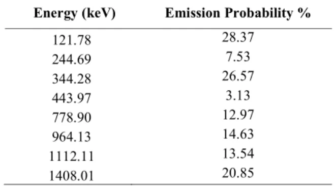
where N(E) is the number of counts in the full.energy peak which can be obtained using Genie 2000 software, T is the measuring time (in second), P(E) is the photon emission probability at energy E, AS is the radionuclide activity and Ci are the correction factors due to dead time and radionuclide decay. Table 5 shows photon energies and photon emission probabilities for 152Eu used in our measurements that are available on the IAEA website. In these measurements of low activity sources, the dead time was less than 3%, so the corresponding factor was obtained simply using ADC live time. The acquisition time was long enough to get statistical uncertainties of the net peak areas smaller than 1%. The background subtraction was done. The decay correction Cd for the calibration source from the reference time to the run time was given by:
T
d e
C = λ (35) where λ is the decay constant and TT is the interval between the source activity reference time and the measurement time.
Table 5. Photon Energies and Photon Emission Probabilities for 152Eu which used in the Current Measurements.
Energy (keV) Emission Probability %
121.78 28.37
244.69 7.53
344.28 26.57
443.97 3.13
778.90 12.97
964.13 14.63
1112.11 13.54
1408.01 20.85
2 2 2 2 2 2
N P
A
N P
A σ
ε σ ε σ ε ε
σε
∂
∂ + ∂ ∂ + ∂ ∂
= (36)
where σA, σP and σN are the uncertainties associated with the quantities AS,
P(E) and N(E) respectively. Tables 6 and 7 show the comparison between the calculated (with and without Sself) and the measured full.energy peak efficiency values of the co.axial HPGe detector for spherical sources placed at the end cap of the detector with volume 113 mL and 179.5 mL respectively, where the percentage deviations between the calculated (with and without Sself) and the measured full.energy peak efficiency values are calculated by:
100 %
with with
1 ×
− =
− −
self self
S cal
meas S
cal
ε
ε ε
(37)
100 %
without without
2 ×
− =
− −
self self
S cal
meas S
cal
ε
ε ε
(38)
where
self
S cal−with
ε ,
self
S cal−without
ε , and εmeasare the calculated with/without self.attenuation factor and experimentally measured efficiencies, respectively.
The discrepancies between calculated with Sself and measured values were found to be less than (2.5%) while, between calculated without Sself and measured values were found to be less than (16%). Obviously, the non.inclusion of the self. attenuation factor in the calculations caused an increase in the full energy peak efficiency values. So to get correct results; the self.attenuation factor must be taken into consideration. Also, Tables 6 and 7 show that, the source self. attenuation is more effective with large sources where the photon has travelled a larger distance within a source matrix, so that, the probability of getting it absorbed is higher and hence the attenuation is stronger. Its effect decreases by decreasing the volume, since the distance travelled by the photon within the source matrix is shorter.
Table 6. Comparison between the Calculated (with and without Sself ) and the Measured Full Energy Peak Efficiency Values of a Co axial HPGe Detector
for a Spherical Source (113 mL) Placed at the End Cap of the Detector.
Energy
(keV) Measured
Calculated
with Sself
@1%
Calculated
without Sself
@2%
Table 7. Comparison between the Calculated (with and without Sself ) and the Measured Full Energy Peak Efficiency Values of a Co axial HPGe Detector
for a Spherical Source (179.5 mL) Placed at the End Cap of the Detector.
Energy
(keV) Measured
Calculated
with Sself
@1%
Calculated
without Sself
@2%
121.78 1.978E.02 1.985E.02 0.38 2.328E.02 15.04 244.69 1.343E.02 1.345E.02 0.13 1.530E.02 12.19 344.28 1.038E.02 1.046E.02 0.78 1.172E.02 11.43 443.97 7.576E.03 7.552E.03 .0.32 8.374E.03 9.53 778.90 3.006E.03 3.038E.03 1.04 3.293E.03 8.70 964.13 2.195E.03 2.204E.03 0.41 2.371E.03 7.41 1112.11 1.796E.03 1.800E.03 0.23 1.927E.03 6.79 1408.01 1.306E.03 1.317E.03 0.78 1.398E.03 6.58
5. Conclusions
This work presents a new analytical approach for calculating the full energy peak efficiency of HPGe detector; this includes the separate calculation of the factors related to photon attenuation in the detector end cap, dead layer, source container and the self.attenuation of the source matrix has been introduced. The examination of the present results as given in tables reflects the importance of considering the self.attenuation factor in studying the efficiency of any detector using spherical sources and shows a great possibility for calibration of HPGe detectors.
Acknowledgment
The authors would like to express their sincere thanks to Prof. Dr. Mahmoud. I. Abbas, Faculty of Science, Alexandria University, for the very valuable professional guidance in the area of radiation physics and for his fruitful scientific collaborations on this topic.
The corresponding author would like to introduce a special thanks to The Physikalisch.Technische Bundesanstalt (PTB) in Braunschweig, Berlin, Germany for fruitful help in preparing the homemade volumetric sources.
References
1. Korun, M. (2002). Measurement of the average path length of Gamma.rays in samples using scattered radiation. Applied Radiation and Isotopes, 56(1.2), 77.83.
2. Lippert, J. (1983). Detector.efficiency calculation based on point.source measurement. Applied Radiation and Isotopes, 34(8), 1097.1103.
3. Moens, L.; and Hoste, J. (1983). Calculation of the peak efficiency of high.purity Germanium detectors. Applied Radiation and Isotopes, 34(8), 1085.1095. 4. Haase, G.; Tait, D.; and Wiechon, A. (1993). Application of new Monte
Physics Research Section A: Accelerators, Spectrometers, Detectors and Associated Equipment, 336(1.2), 206.214.
5. Wang, T..K.; Mar, W..Y.; Ying, T..H.; Liao, C..H.; and Tseng, C..L. (1995). HPGe detector absolute.peak.efficiency calibration by using the ESOLAN program. Applied Radiation and Isotopes, 46(9), 933.944.
6. Wang, T..K.; Mar, W..Y.; Ying, T..H.; Tseng, C..H.; Liao, C..H.; and Wang, M..Y. (1997). HPGe detector efficiency calibration for extended cylinder and Marinelli.beaker sources using the ESOLAN program. Applied Radiation and Isotopes, 48(1), 83.95.
7. Sima, O.; and Arnold, D. (1996). Self.attenuation and coincidence summing corrections calculated by Monte Carlo simulations for Gamma.spectrometric measurements with well.type Germanium detectors. Applied Radiation and Isotopes, 47(9.10), 889.893.
8. Abbas, M.I. (2001). A direct mathematical method to calculate the efficiencies of a parallelepiped detector for an arbitrarily positioned point source. Radiation Physics and Chemistry, 60(1.2), 3.9.
9. Abbas, M.I. (2001). Analytical formulae for well.type NaI(Tl) and HPGe detectors efficiency computation. Applied Radiation and Isotopes, 55(2), 245.252.
10. Abbas, M.I.; and Selim,Y.S. (2002). Calculation of relative full.energy peak efficiencies of well.type detectors. Nuclear Instruments and Methods in Physics Research Section A: Accelerators, Spectrometers, Detectors and Associated Equipment, 480(2.3), 651.657.
11. Selim, Y.S.; Abbas, M.I.; and Fawzy, M.A. (1998). Analytical calculation of the efficiencies of Gamma scintillators. Part I: Total efficiency of coaxial disk sources. Radiation Physics and Chemistry, 53(6), 589.592.
12. Selim, Y.S.; and Abbas, M.I. (2000). Analytical calculations of Gamma scintillators efficiencies. Part II: Total efficiency for wide coaxial disk sources. Radiation Physics and Chemistry, 58(1), 15.19.
13. Abbas, M.I. (2006). HPGe detector absolute full.energy peak efficiency calibration including coincidence correction for circular disc sources. Journal of Physics D: Applied Physics, 39(18), 3952.3958.
14. Abbas, M.I.; Nafee, S.S.; and Selim, Y.S. (2006). Calibration of cylindrical detectors using a simplified theoretical approach. Applied Radiation and Isotopes, 64(9), 1057.1064.
15. Pibida, L.; Nafee, S.S.; Unterweger, M.; Hammond, M.M.; Karam, L.; and Abbas, M.I. (2007). Calibration of HPGe Gamma.ray detectors for measurement of radio.active noble gas sources. Applied Radiation and Isotopes, 65(2), 225.233.
16. Nafee, S.S.; and Abbas, M.I. (2008). Calibration of closed.end HPGe detectors using bar (parallelepiped) sources. Nuclear Instruments and Methods in Physics Research Section A: Accelerators, Spectrometers, Detectors and Associated Equipment, 592(1.2), 80.87.
17. Hamzawy, A. (2004). Accurate direct mathematical determination of the efficiencies of Gamma detectors arising from radioactive sources of Different shapes. Ph.D. Dissertation. Alexandria University, Egypt.
![Table 1. Values of Polar and Azimuthal Angles Based on the Source to Detector Configuration [13]](https://thumb-eu.123doks.com/thumbv2/123dok_br/17036214.233372/5.918.196.598.240.546/table-values-polar-azimuthal-angles-source-detector-configuration.webp)