FUNDAÇÃO GETÚLIO VARGAS
ESCOLA DE ECONOMIA DE EMPRESAS DE SÃO PAULO
Joana Colarinha Vieira
International Portfolio Diversification: Evidence from Emerging Markets
FUNDAÇÃO GETÚLIO VARGAS
ESCOLA DE ECONOMIA DE EMPRESAS DE SÃO PAULO
Joana Colarinha Vieira
International Portfolio Diversification: Evidence from Emerging Markets
SÃO PAULO 2015
Dissertação apresentada à Escola de Economia de Empresas de São Paulo da Fundação Getúlio Vargas, como requisito para obtenção do título de Mestre Profissional em Economia.
Campo do Conhecimento: International Master in Finance
Orientador Prof. Dr. João Mergulhão (advisor)
Vieira, Joana.
International Portfolio Diversification: Evidence from Emerging Markets / Joana Vieira. - 2015.
56 f.
Orientador: João Mergulhão.
Dissertação (MPFE) - Escola de Economia de São Paulo.
1. Investimentos estrangeiros. 2. Mercados emergentes. 3. Risco (Economia. 4. Finanças internacionais I. Mergulhão, João. II. Dissertação (MPFE) - Escola de Economia de São Paulo. III. Título.
Joana Colarinha Vieira
International Portfolio Diversification: Evidence from Emerging Markets
Dissertação apresentada à Escola de Economia de Empresas de São Paulo da Fundação Getúlio Vargas, como requisito para obtenção do título de Mestre Profissional em Economia.
Campo do Conhecimento: International Master in Finance
Data de Aprovação: 25/09/2015.
Banca Examinadora:
______________________________ ___
Prof. Dr. João Mergulhão
______________________________ ___
Prof. Dr. Martijn Boons
ABSTRACT
Taking into account previous research we could assume to be beneficial to diversify
investments in emerging economies. We investigate in the paper International Portfolio
Diversification: evidence from Emerging Markets if it still holds true, given the
assumption of larger world markets integration.
Our results suggest a wide spread positive time-varying correlations of emerging and developed markets. However, pair-wise cross-country correlations gave evidence that emerging markets have low integration with developed markets. Consequently, we evaluate out-of-sample performance of a portfolio with emerging equity countries, confirming the initial statement that it has a better a risk-adjusted performance over a purely developed markets portfolio.
Keywords: international portfolio diversification; pairwise correlation; dynamic
RESUMO
Considerando estudos anteriores, podemos assumir ser benéfico diversificar os
investimentos em economias emergentes. No estudo Diversificação do Portfolio
Internacional: evidência de mercados emergentes, investigamos se o mesmo
ainda se verifica, tendo em conta o pressuposto de uma maior integração
global dos mercados.
Os nossos resultados sugerem correlações positivas ao longo do tempo de economias emergentes com mercados desenvolvidos. Contudo, as correlações entre países evidenciam que países emergentes ainda estão pouco integrados com os países
desenvolvidos. Consequentemente, avaliamos o desempenho de um portfolio fora da amostra, com acções de país emergentes, confirmando o pressuposto inicial de que este apresenta um desempenho, ajustado ao risco, ligeiramente superior a um portfolio puramente constituído com acções de mercados desenvolvidos.
Palavras Chave:
diversificação do portfolio internacional; correlação aos pares;
TABLE OF CONTENTS
Index of Figures
Figure 1: Dynamic Conditional Correlation between the MSCI Developed Markets Equity Index returns and the MSCI regional Equity Indexes returns (Emerging; Emerging Latin America; Emerging Asia; Emerging EMEA) ... 35
Figure 2: Dynamic Conditional Correlation between the returns of the MSCi Developed Markets Equity Index, and MSCi China, India, Taiwan Equity Indexes returns ... 37 Figure 3: Dynamic Conditional Correlation between the returns of the MSCi Developed Markets Equity Index, and MSCi Indonesia, Malaysia, Thailand Equity Indexes returns ... 37 Figure 4: Dynamic Conditional Correlation between the returns of the MSCi Developed Markets Equity Index, and MSCi Korea, Philippines Equity Indexes returns ... 38 Figure 5: Dynamic Conditional Correlation between the returns of the MSCi Developed Markets Equity Index, and MSCi Czech Republic, Greece, Hungary Equity Indexes returns ... 39
Figure 6: Dynamic Conditional Correlation between the returns of the MSCi Developed Markets Equity Index, and MSCi Poland, Russia Equity Indexes returns ... 39 Figure 7: Dynamic Conditional Correlation between the returns of the MSCi Developed Markets Equity Index, and five MSCi Egypt, South Africa and Turkey Equity Indexes returns ... 40 Figure 8: Dynamic Conditional Correlation between the returns of the MSCi Developed Markets Equity Index, and MSCi Chile, Mexico and Brazil Equity Indexes returns ... 41 Figure 9: Dynamic Conditional Correlation between the returns of the MSCi Developed Markets Equity Index, and five MSCi Peru and Colombia Equity Indexes returns41
Figure 10 – Mean Variance Efficient Frontier for 21 Emerging Countries and 23 Developed Countries Equity Indices, January 29, 1999 to November 21, 2014 .... 48
Index of Tables
Table 1: ETF Universe ... 20 Table 2: Descriptive Statistics for monthly MSCI equity indexes returns. ... 30
Table 3: Descriptive Statistics for monthly ETFs equity indexes returns, for the full sample period. ... 32 Table 4: Descriptive Statistics for monthly ETFs equity indexes returns, for the
out-of-sample period. ... 33
Table 13: Summary of unconditional correlations for the regional MSCI’ indices ... 43 Table 14: Heat color map of the cross-country correlations between 21 MSCI Emerging Countries indices and 5 MSCI regional indices ... 45
Table 16: International Portfolios (ex-post) ... 50
Table 5: average of the DCC coefficients, between the returns of the MSCi Developed Markets Equity Index, and MSCi China, India, Taiwan Equity Indexes returns, for each year ... 54
Table 6: average of the DCC coefficients, between the returns of the MSCi Developed Markets Equity Index, and MSCi Indonesia, Malaysia, Thailand Equity Indexes returns, for each year ... 54
Table 7: average of the DCC coefficients, between the returns of the MSCi Developed Markets Equity Index, and MSCi Korea, Philippines Equity Indexes returns, for each year ... 54
Table 8: average of the DCC coefficients, between the returns of the MSCi Developed Markets Equity Index, and MSCi Czech Republic, Greece, Hungary Equity Indexes returns, for each year ... 54
INDEX
1. Introduction ... 10
2. Literature Review ... 12
3. Data and Methodology ... 18
3.1 Data ... 18
3.2 Methodology ... 21
3.2.1 Dynamic Conditional Correlation (DCC) model ... 21
3.2.2 Pairwise unconditional correlations ... 23
3.2.3 Mean-Variance Model ... 23
3.2.4 The Naive Portfolio ... 25
3.2.5 The Risk Parity Portfolio ... 25
3.2.6 Out of Sample evaluation ... 25
3.2.7 Performance Measures ... 26
4. Results ... 28
4.1 Descriptive Statistics of returns ... 28
4.2 Dynamic Conditional Correlations ... 34
4.3 Pairwise Correlations ... 44
4.4 Mean-variance model ... 47
4.5 International ETFs Portfolios ... 48
5. Conclusion ... 50
6. References ... 52
1. Introduction
One of the most important classical arguments in favor of international diversification is to benefit from the lower correlations among stocks in different markets. When correlations within equity returns are high, it is likely that when one stock loses other stocks may loose as well. Hence, potential gains from diversification are greater when correlation between stock returns is low. Solnik (1976) provided evidence that a globally diversified portfolio could half the risk of a diversified portfolio of U.S. stocks.
Furthermore, the potential diversification gains are substantial when developing countries are included in the set of investment opportunities. Literature on Emerging markets finance describes these markets as being highly volatile with impressive expected returns (Mullin 1993, Santis et al. 1997). Moreover, correlations of these equity returns with developed countries’ equity returns are low. Consequently, it may be possible to decrease portfolio risk by diversifying into emerging markets.
In his seminal article Campbell R. Harvey (1995) provided the first comprehensive
analysis of 20 new equity markets in emerging economies, claiming that given the low
correlations among emerging with developed market returns (1986-1992), the inclusion
of emerging market assets in a mean-variance efficient portfolio significantly reduces
portfolio volatility and increases expected returns.
However, Shawky et al. (1997) point towards a reduction of the potential gains from
international diversification (1990-1995), due to the increased worldwide integration of
financial markets, which might have caused stronger co-movements among
Taking in consideration the debate motivated by the scope of previous research, this
paper aims to analyze if it might still be interesting for investors in developed markets,
in current days, to diversify their equity portfolios into developing economies.
For this purpose we begin by investigate the recent level of international stock market
correlations for the elapsed time of 1995 until 2014, exploring an MSCI dataset of
emerging and developed markets. We further evaluate if correlations are changing and increasing over the same period using the Dynamic Conditional Correlation model (DCC), with a particular focus on the behavior of returns correlations during the subprime crisis period. Lastly, we have an empirical analysis of Exchange Traded Funds (ETFs) portfolio performance, with and without emerging markets stocks.
In this project we analyze seventeen developed countries equity ETFs and sixteen emerging countries equity ETFs between 1996 and 2015. Given that ETFs are relatively new, the number of ETFs that we could choose from is limited.
The portfolios’ allocations are based on the historical averages of the expected returns, and variances of the ETFs indices collected. For each case, two strategies are examined: (i) risk parity portfolio and (ii) equally weighted portfolio. The performance of each portfolio is evaluated on a 60-month rolling window, out-of-sample basis, over the 30/04/2001 to 27/02/2015 period. That is, the first allocation is based on data from 30/04/1996 to 30/03/2001. The portfolio is re-optimized at each point in time.
The study is organized as follows. In the first section is provided a review of some selected literature relevant to the study. The second section describes the data used in the study. Empirical results are discussed in the subsequent section. Finally, the last section provides a conclusion and a summary of the findings of this study.
2. Literature Review
Emerging stock markets are especially known for having higher average returns, due to a superior economic growth during economical expansionary cycles, and bigger volatilities, associated to more unstable political, economical and financial environments. Moreover, global risk factors are expected to have minimal, or even no influence in their performance, explaining the low returns correlations with other emerging markets and developed markets (Pajuste et al 2000).
country risk is a good determinant of diversification benefits, with countries with greater country risk having the higher potential benefits coming from global diversification. However, their findings also show that diversification benefits have decreased over the sample period 1985-2002. The reduction in diversification benefits seems to be linked to an improvement in the country risk over time.
Also, Salomons et al. (2003) tested whether the perceived risk is reflected in larger equity risk premium (ERP) for emerging markets, finding that when comparing ex post ERP for emerging markets to developed markets, the ERP is significantly higher in emerging markets.
Given these results, developing markets appear to represent interesting investment opportunities for global investors improving expected return and lower risk.
However, in recent years, financial markets have become more integrated, which leads to greater correlations between stock markets in different countries and an implied reduction of benefits from international diversification. Eiling et al (2006) concluded that equity markets around the world are becoming increasingly interconnected. In a sample of 32 emerging markets, from Q3 1991 to Q2 2009, they found significant positive trends in cross-country correlations within regions, correlations across emerging regions and correlations between emerging markets and the rest of the world. The authors still traced increased average correlations among emerging market regions from less than 0,1 in the early 1990s to close to 0,8 in recent years.
Financial crisis are one of the main factors responsible for the variation of market correlations and consequent increase, discouraging then international diversification.
Moreover, literature documents that emerging countries are more vulnerable to crisis due to their underdeveloped financial markets, which are also not so good news for investors diversifying in these markets, although developed countries are also affected. Crisis as the Wall Street crash in 1987, the European monetary system collapse in 1992, the 1994 Mexican pesos crisis, the 1997 “Asian Flu”, the 1998 “Russian Cold”, the 1999 Brazilian devaluation, the 2000 Internet bubble burst, the Argentinian default crisis in July 2001, and the recent American mortgage market crisis, have affected financial markets worldwide and resulted in catastrophic losses. All starts with a country-specific shock, which spreads rapidly to other markets (Billio et al. 2009). Researchers as Forbes and Rigobon (2000), Bae et al. (2003), Eichengreen et al. (1995, 1996) have attempted to elucidate the rational for these financial setbacks and the mechanisms of their global spread. An international propagation phenomenon of shocks also referred as “contagion”.
According to the World Bank’s framework we can distinguish three distinctive definitions of contagion1:
1.Broad definition: whereby contagion is identified as a general process of shock transmission across countries. A process supposed to work during calm as well as in crisis periods. Accordingly, a contagion is associated not only with negative shocks but also with positive spillover effects;
1
2.Restrictive Definition: referring to contagion as a propagation of shocks between two countries (or group of countries) in excess of what should be expected by fundamentals and considering the co-movements triggered by ordinary shocks.
3.Very restrictive definition: in this case contagion should be interpreted as the change in the transmission mechanisms that takes place during turn oil period. For example, the latter can be inferred by a significant increase in the cross-market correlation. (This is the one adopted by Forbes and Rigobon (2000))
(contagion)2; followed by a second one showing a continued high correlation (herding). Moreover, the authors’ finding of contagion effects during the Asian financial crisis goes against Forbes and Rigobon (2002) conclusion of “no contagion”.
The Dynamic Conditional Correlation analysis has then been widely used to measure the degree of financial contagion. As in these studies, we are applying the Dynamic Conditional Correlation Model (Engle 2002), to analyze the evolution of the correlations between the developed markets MSCI indices and twenty-one emerging countries. Moreover, as correlation coefficients across markets are likely to increase after a bad shock, we access if the same is verified between developed and emerging markets during the 2008 subprime crisis. This analysis more focused on the 2008 crisis was motivated by Valls Pereira et al. (2013) study. The authors state that the comparison of correlations, between the returns of the markets of interest, before and after the event theoretically responsible for triggering the financial crisis, is a very intuitive way of assessing the contagion presence. King and Wadhwani (1990) also employ this method to examine the 1987 American crisis (Wall Street Crash), finding superior correlations among markets of the United States, the United Kingdom and Japan after this event. However, we can also find authors providing evidence of no contagion across different economies, after crisis events (Lee and Kim (1993), Forbes
2
and Rigobon (2002)).
This paper concludes with the evaluation of equity country ETFs. There are a few studies in the literature examining the performance of country equity ETFs portfolios. Huang et al., 2011 found that investors investing in ETFs of foreign markets (for the period 2003-2009) will have no performance difference from those who invest in a more direct way (only in the S&P500). In Petronio et al., 2014 we can find an analysis of the main ETF markets (U.S. and European), for the period 2006-2012, and examine the portfolio selection problem. A different study compares the performance of a portfolio consisting of exchange-traded funds (ETFs) with that of the overall market, exemplified by the Topix Index (2008-2009). Kono et al. 2011, concludes that an optimal ETF portfolio can outperform an overall market index when performance is measured using the Sharpe ratio.
model across seven different empirical datasets of the global equities universe. The authors also emphasize that when evaluating the performance of a particular strategy for optimal asset allocation the 1/n rule, should serve at least as a first obvious benchmark. Supported by this discussion we propose the following research questions:
1st question: How have emerging countries’ time-varying correlations with developed markets been changing in the last 15 years?
2nd question: What are the average historical correlations among international markets, for the same period, ranging from 1999 to 2014?
3rd question: Is a portfolio with emerging equity country ETFs outperforming a portfolio with only developed equity country ETFs, for the period 1996 to 2015?
The main contribution of the current paper should rely on the study of an innovative dataset, analyzing its correlations and benefits according to the type of portfolio combinations adopted, offering a first comparison for the selected sample in a recent period.
3. Data and Methodology
3.1 Data
index values, corresponding to the emerging markets sample refer to the following indexes: MSCI Equity Indexes of Peru, Chile, Colombia, Mexico, Brazil, China, India, Indonesia, Korea, Malaysia, Philippines, Taiwan, Thailand, Czech Republic, Egypt, Greece, Hungary, Poland, Russia, South Africa, Turkey. While the collected index values, corresponding to the developed markets sample refer to the MSCI indexes of Norway, Portugal, Singapore, Spain, Sweden, Switzerland, United Kingdom, USA, Australia, Austria, Belgium, Canada, Denmark, Finland, France, Germany, Hong Kong, Ireland, Israel, Italy, Japan, Netherlands, New Zealand. The country selection for both samples, emerging and developed markets, was done according to the constitution of the MSCI Emerging Markets Index and MSCI Developed Markets Index. Qatar and United Arab Emirates were excluded from the sample for not having enough data available for the period of this study. Considering the comparison of correlations between regions and the world index three MSCI indices were collected for the emerging markets of Latin America, Asia, Europe/Middle East/Africa; two MSCI indices for emerging and developed markets, and, finally, the MSCI world index.
The sample period goes from 29 of January 1999 to 21 of November 2014, using 191observations for each index. The time frame was defined in a way that it could be used the largest amount of data as possible, regarding the availability of prices for each index. The selected Markets follow the categorization of Emerging Markets or Developed Markets according to the MSCI classification, as of October 2013.
period of study ranging from 29/03/96 until 27/02/15. The table below provides the description of the ETFs indexes collected.
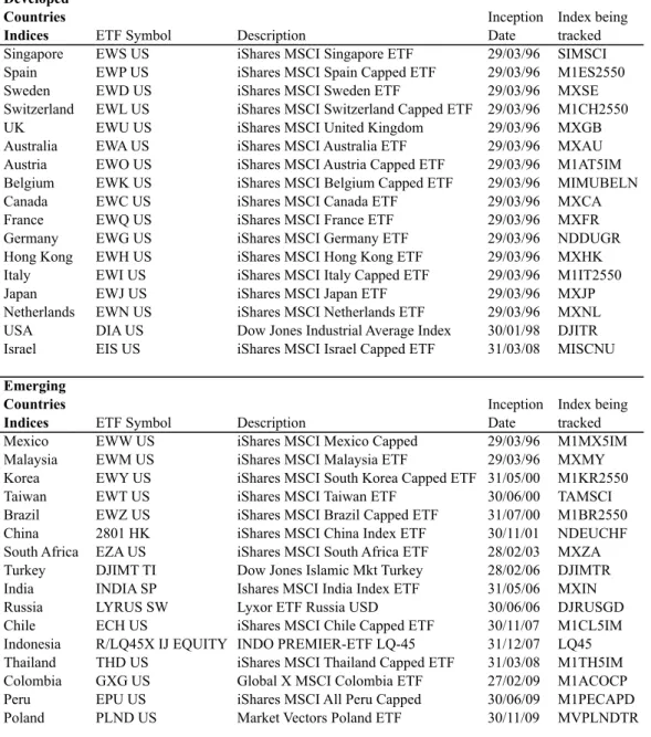
Table 1: ETF Universe
The benchmark being used is the MSCi World Index (MXWD). The risk-free rate considered in our study is the US three-month Treasury Bill obtained from the Federal Reserve Economic Data web database. All strategies are developed and implemented in U.S. dollar terms. This assumes that no currency hedging takes place.
Developed Countries
Indices ETF Symbol Description
Inception Date
Index being tracked
Singapore EWS US iShares MSCI Singapore ETF 29/03/96 SIMSCI
Spain EWP US iShares MSCI Spain Capped ETF 29/03/96 M1ES2550
Sweden EWD US iShares MSCI Sweden ETF 29/03/96 MXSE
Switzerland EWL US iShares MSCI Switzerland Capped ETF 29/03/96 M1CH2550
UK EWU US iShares MSCI United Kingdom 29/03/96 MXGB
Australia EWA US iShares MSCI Australia ETF 29/03/96 MXAU
Austria EWO US iShares MSCI Austria Capped ETF 29/03/96 M1AT5IM Belgium EWK US iShares MSCI Belgium Capped ETF 29/03/96 MIMUBELN
Canada EWC US iShares MSCI Canada ETF 29/03/96 MXCA
France EWQ US iShares MSCI France ETF 29/03/96 MXFR
Germany EWG US iShares MSCI Germany ETF 29/03/96 NDDUGR
Hong Kong EWH US iShares MSCI Hong Kong ETF 29/03/96 MXHK
Italy EWI US iShares MSCI Italy Capped ETF 29/03/96 M1IT2550
Japan EWJ US iShares MSCI Japan ETF 29/03/96 MXJP
Netherlands EWN US iShares MSCI Netherlands ETF 29/03/96 MXNL USA DIA US Dow Jones Industrial Average Index 30/01/98 DJITR
Israel EIS US iShares MSCI Israel Capped ETF 31/03/08 MISCNU
Emerging Countries
Indices ETF Symbol Description
Inception Date
Index being tracked
Mexico EWW US iShares MSCI Mexico Capped 29/03/96 M1MX5IM
Malaysia EWM US iShares MSCI Malaysia ETF 29/03/96 MXMY
Korea EWY US iShares MSCI South Korea Capped ETF 31/05/00 M1KR2550
Taiwan EWT US iShares MSCI Taiwan ETF 30/06/00 TAMSCI
Brazil EWZ US iShares MSCI Brazil Capped ETF 31/07/00 M1BR2550
China 2801 HK iShares MSCI China Index ETF 30/11/01 NDEUCHF
South Africa EZA US iShares MSCI South Africa ETF 28/02/03 MXZA Turkey DJIMT TI Dow Jones Islamic Mkt Turkey 28/02/06 DJIMTR
India INDIA SP Ishares MSCI India Index ETF 31/05/06 MXIN
Russia LYRUS SW Lyxor ETF Russia USD 30/06/06 DJRUSGD
Chile ECH US iShares MSCI Chile Capped ETF 30/11/07 M1CL5IM
Indonesia R/LQ45X IJ EQUITY INDO PREMIER-ETF LQ-45 31/12/07 LQ45 Thailand THD US iShares MSCI Thailand Capped ETF 31/03/08 M1TH5IM
Colombia GXG US Global X MSCI Colombia ETF 27/02/09 M1ACOCP
Peru EPU US iShares MSCI All Peru Capped 30/06/09 M1PECAPD
3.2 Methodology
As previously mentioned, this paper addresses three different questions, with distinctive methods for each one.
3.2.1 Dynamic Conditional Correlation (DCC) model
The 1st research question refers to the analysis of time-varying correlations changes, between developed and emerging markets, in the last 15 years. The fluctuations of the correlations are modeled according to the DCC Model, as proposed by Engle (2002) and Tse and Tsui (2002) as an extension to the CCC model. The DCC model is preferred to the Constant Conditional Correlation model because it corrects its main defect on assuming constant correlations over time, which is not supported by empirical evidence. Both models belong to the family of multivariate GARCH models. To describe the DCC model as proposed by Engle (2002) we start by specifying the multivariate conditional variance:
𝐻! = 𝐷!𝑅!𝐷! (1)
Where 𝐷! is the (n x n) diagonal matrix of time-varying standard deviations from univariare GARCH models with ℎ!!,! on the ith diagonal, i = 1,2, …, n; 𝑅! is the (n x
n) time-varying correlation matrix. According to the DCC model the conditional covariance matrix 𝐻! is estimated in two steps. Firstly, univariate volatility models are
fitted for each of the stock returns and are obtained the estimates of ℎ!!,! . Secondly,
stock-return residuals are transformed by their estimated standard deviations from the first stage 𝑢!,! = 𝜀!,! / ℎ!!,! and 𝑢!,! is then used to estimate the parameters of the
𝑄!= (1 - 𝛼 - 𝛽)𝑄 + 𝛼𝑢!!!𝑢′!!! + 𝛽𝑄!!! (2) Where 𝑄! = (𝑞!",!) is the n x n time-varying covariance matrix of 𝑢!, 𝑄 = E 𝑢!𝑢′! is the
n x n unconditional variance matrix of 𝑢!, and 𝛼 and 𝛽 are nonnegative scalar
parameters satisfying (𝛼+ 𝛽) < 1. Because 𝑄! does not generally have ones on the diagonal, we scale it to obtain a proper correlation matrix 𝑅!. Therefore,
𝑅!= (𝑑𝑖𝑎𝑔 𝑄! )!!/! 𝑄!(𝑑𝑖𝑎𝑔 𝑄! )!!/! (3)
Where (𝑑𝑖𝑎𝑔 𝑄! )!!/! = diag (1/ 𝑞!!,!, …, 1/ 𝑞!!,!).
In Equation 3, 𝑅! is a correlation matrix with ones on the diagonal and off-diagonal elements less than one in absolute value, as long as 𝑄! is positive definite. The DCC model can be estimated by maximum likelihood breaking the log-likelihood function into two parts. First we estimate the parameters that determine the univariate volatilities and in a second phase we estimate the parameters that determine the correlations. Let 𝜃 denote the parameters in 𝐷!, and 𝜙 the parameters in 𝑅!, then the log-likelihood fund is:
𝑙! (𝜃,𝜙)= −!
! (
𝑛log 2𝜋 +𝑙𝑜𝑔 𝐷! ! !
!!! +𝜀!!𝐷!!!𝜀!) +
− !
! (log 𝑅!
+𝑢!!𝑅!!!𝑢!−𝑢!!𝑢!)
!
!!! .
(4)
The volatility can then be found in the first part of the likelihood function in Equation (4), obtained by the sum of individual GARCH likelihoods. The log-likelihood function can be maximized in the first step over the parameters in 𝐷!. Once we have the
3.2.2 Pairwise unconditional correlations
Assuming the theoretical model of portfolio selection, the degree to which diversification can reduce risk depends upon the correlations among security returns and consequently diversification could eliminate risk if the returns are not correlated.
Motivated by the fact that equity markets around the world are becoming increasingly interconnected we are studying the cross-country correlations. This way, to attend the question on what are the levels of correlation among international markets, for a more recent period, we calculated two different matrices containing the pairwise Pearson’s linear correlation coefficient between each pair of indices in order to measure the co-movements between each two returns series. The period under analysis goes from January 29th, 1999 to November 21st, 2014. In first place come the correlation coefficients for 27 MSCI Emerging Countries indices with regional indices and the world index (Table 14.1 in appendix). Follows the correlations between 27 MSCI Emerging Countries indices and 23 MSCI Developed Countries indices (table 15.1 in appendix). The respective p-values for Pearson’s correlation were computed as well. Testing the null of no correlation, using a Student’s t distribution for a transformation of the correlation. Additionally, we complement the cross-country correlations analysis with a particular focus on the 2008 subprime crisis. We employ a sub-sample analysis to the unconditional cross-market correlation coefficients in the pre- and post-crisis periods. If the correlation coefficient increases significantly during the crisis, this may imply a statistically higher degree of cross-market linkages (Kim et al. 2015).
3.2.3 Mean-Variance Model
paper (1972) methodology. When deriving efficient frontiers, we choose the weights that would minimize the portfolio variance σ! ≡ ω′Ω!!ω, subject to the budget constraint ω′e= 1 (e unit vector) and a given level of expected portfolio return ω!ER=
µμp. The optimal weights were obtained using the (n x n) covariance matrix of returns Ω, the expected returns on the risky assets ER (n x 1) and the chosen mean portfolio return ERp≡µμp. The minimum variance portfolio has: var(Rp)= ω′Ω!!ω, where ω is the (n x1 ) vector of optimal proportions held in the risky assets calculated as follows:
𝜔 =Ω!! 𝐸𝑅 𝐶𝜇𝑝−𝐵
+𝑒(𝐴−𝐵𝜇𝑝)
(𝐴𝐶− 𝐵!)
(5)
A = (ER’)Ω!! (ER) (6)
B= (ER’)Ω!! e (7)
C= e’Ω!! e (8)
To answer all the proposed questions, monthly index returns are calculated based on the following logarithmic difference:
𝑅𝑡= log(𝑃𝑡/𝑃𝑡−1) (9)
In order to dimension the risk level, volatility is calculated through the standard deviation of the returns given by:
s = (!! !! (𝑥𝑖−𝑥
!! )^2)
3.2.4 The Naive Portfolio
One of the weighting methodologies under analysis on this study refers to the naive strategy. As described in DeMiguel, the “ew” or “1/N” strategy gives the weight of 1/N to each of the N risky assets. Moreover, this strategy does not imply any optimization or estimation and totally ignores the data.
3.2.5 The Risk Parity Portfolio
The portfolios are also being weighted according to the risk parity strategy, in order to evaluate which method allows to a superior risk-adjusted performance.
This weighting methodology aims to equalize risk contributions from the different components of the portfolio, so that no asset contributes more than its peers to the total risk of the portfolio.3
So, the analytic solution under which we find the weight allocated to each component i is given by:
𝑥! = !!!!
!
!!! ! !!!
, (11)
Consequently, as higher the volatility of a component is, the lower its weight in the ERC portfolio. We are taking the constraint of no short selling, 0 ≤𝑥≤ 1.
3.2.6 Out of Sample evaluation
The analysis of the aforementioned models follows a “rolling-sample” approach. As in DeMiguel, we choose an estimation window of length M = 60 for a T – month-long
3
dataset of asset returns. 4So, in each month t, and starting from t = M + 1, we take the data from the previous M months to estimate the parameters needed to determine the relative portfolio weights for each strategy. These weights are then used to compute the return for the month t +1. Then, we repeat this procedure for the next period, by including the data for the new date and dropping the data for the earliest period. We continue doing this until the end of the data set is reached. At the end we have a series of T – M monthly out-of-sample returns generated by each of the portfolio strategies. Moreover, both strategies are unconditional due to how we choose expected returns, and variances. By using the average returns over the previous 60 months, although the mean returns change through time as the 60-month window moves, we are assuming that the best forecast of the equity returns are its past average. This implies that there is no other relevant information to forecast the next month stock price besides the previous price. In what refers to the variances, these are assumed to be unconditional over the previous 60 months. All strategies are developed and implemented in U.S. dollar terms, no currency hedging is taking place.
3.2.7 Performance Measures
For each strategy and each dataset we compute four different performance measures. First we measure the out-of-sample Sharpe ratio of strategy k, defined by Sharpe (1994) as:
Sharpe = !"! !"
!" ,
(12)
where 𝑅𝑝 is the annualised return, 𝑅𝑓is the annualized risk-free rate and 𝜎P is the
4
volatility of the returns.
Second we calculate the Modified Sharpe ratio (MSR) as defined by Gregoriou and Gueyie (2003):
Modified Sharpe Ratio = !"!!"
!"#$%
(13)
This measure allows to take into account the higher moments of the distribution skewness (S) and excess kurtosis (K). So the MSR increases the complexity of the Sharpe ratio in the sense that it captures higher moments in the risk measure of the denominator, by using the Cornish-Fisher expansion.
Cornish-Fisher expansion:
𝑧!=𝑧! + !
!(𝑧!
! - 1)S + ! !" (𝑧!
!
- 3𝑧!)(K – 3) - !
!"(2𝑧!
!
-5𝑧!)𝑆! (14)
where the Modified VaR (MVARp) measure is given by:
Modified VaRp (1-𝛼) = abs (-(𝜇 + 𝑧!𝜎) ) (15)
where 𝑧! is the z-statistic corresponding to a one-sided standard normal PDF for 1 − 𝛼
confidence, where 𝛼 is 5%.
The Maximum Drawdown ratio (DD ratio) is given by:
Maximum Drawdown Ratio = !"!!"
!"#!!
(16)
drawdown. The maximum drawdown corresponds to the maximum amount lost from the highest preceding high to the lowest low, during the period that the portfolio has not recuperated its value to that above the last highest high. When the portfolio value recuperates from its losses and achieves a net new high it is said to be out of its drawdown. The input range in this case are the Value Added Monthly Indexes constructed from the monthly returns.
Finally, the Sortino ratio uses the concept of the Minimum Acceptable Return (MAR) in the denominator and in this case it is fixed at 5%. By setting a minimum acceptable rate of return for the investor, the returns are being split into two categories: returns greater than or equal to MAR and returns less than MAR. This measure only uses the downside returns in the calculation so, the higher the Sortino ratio, the better the control of the downside returns, while not being penalized by upside returns.
Sortino = !!!!"# !
! (!!,!!!"#)!
! !!! !"!!"#
(17)
4. Results
4.1 Descriptive Statistics of returns
and out-of-sample period (table 4). The reason why we are analyzing the returns statistics in the full and out-of-sample period is because when constructing the ETFs portfolios we are only allocating the out-of-sample returns.
Concerning the MSCI equity indices being studied, the results for the jarque-bera test show that empirical return distributions are far from a normal distribution, except for Taiwan and Japan MSCI indices. In general terms, all markets have kurtosis higher than 3 (the benchmark value for a normal distribution), suggesting that the series is characterized by leptokurtosis. Hence the distributions of the returns in the markets considered have a greater number of observations in the tails, than what it should be found in a normal distribution.
For the considered period all the average returns revealed to be negative except for Greece (1,04%), Portugal (0,48%) and Italy (0,23%), although the indices for these countries didn’t have the highest levels of volatility, as it would be expected. For example, both Turkey and Russia have standard deviations of 14,64% and 11,52% respectively, while Portugal has a standard deviation of just 6,85%.
Looking to the Emerging Markets MSCI Index the value for average returns is -0,65% and the standard deviation is 6,77%, while the Developed Markets MSCI index has an average return of -0,21%, with a volatility of 4,60%. Resulting that emerging markets seem to have a lower return combined with a larger volatility.
Table 2: Descriptive Statistics for monthly MSCI equity indexes returns.
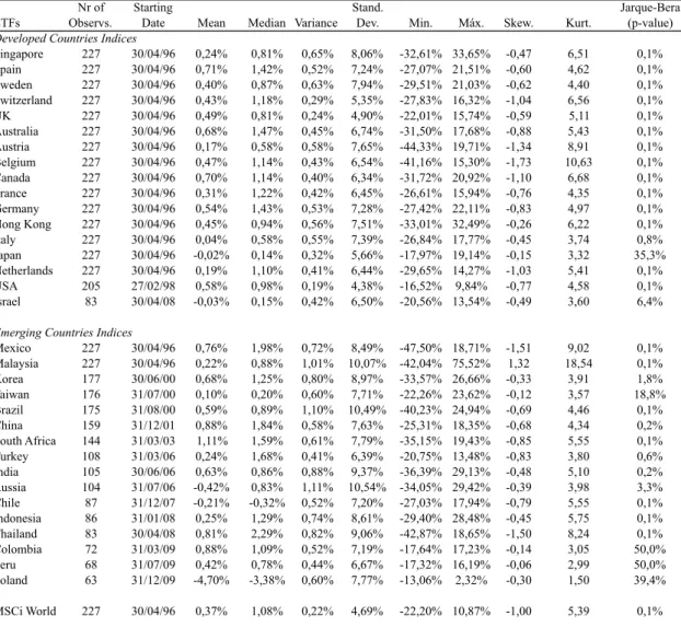
Looking at the results with ETFs sample for the full period (table 3), the jarque-bera test
MSCI
Nr of
Observs. Mean Median Variance Stand.
Dev. Min. Máx. Skew. Kurt.
Jarque-Bera (p-value)
Emerging countries Americas
Peru 191 -1,15% -1,50% 0,73% 8,55% -23,68% 44,70% 0,87 6,53 0,1%
Chile 191 -0,62% -0,70% 0,42% 6,46% -18,29% 29,65% 0,76 5,64 0,1%
Colombia 191 -1,39% -2,08% 0,78% 8,85% -24,20% 33,62% 0,49 4,17 0,3% Mexico 191 -1,01% -1,65% 0,52% 7,18% -16,83% 36,71% 0,91 6,14 0,1% Brazil 191 -0,90% -1,23% 1,10% 10,49% -31,12% 39,08% 0,57 4,74 0,1%
Asia
China 191 -0,49% -0,86% 0,75% 8,65% -38,19% 25,84% 0,11 5,08 0,1%
India 191 -0,93% -1,63% 0,80% 8,92% -31,49% 33,22% 0,41 3,99 0,8%
Indonesia 191 -1,08% -1,59% 1,20% 10,95% -34,18% 48,77% 0,41 5,21 0,1%
Korea 191 -0,79% 0,00% 0,93% 9,66% -30,54% 39,09% 0,21 4,54 0,3%
Malaysia 191 -0,67% -0,81% 0,37% 6,08% -32,86% 19,18% -0,47 6,74 0,1% Philippines 191 -0,42% -0,80% 0,57% 7,54% -21,86% 27,94% 0,30 3,72 3,2% Taiwan 191 -0,18% -0,39% 0,62% 7,85% -25,64% 24,53% 0,07 3,55 22,7% Thailand 191 -0,78% -1,38% 0,91% 9,55% -35,97% 39,93% 0,41 5,53 0,1%
Europe/ Middle East/ Africa
Cz Repub 191 -0,85% -0,98% 0,70% 8,38% -26,91% 34,01% 0,42 4,58 0,1%
Egypt 191 -0,82% -0,82% 0,91% 9,54% -35,51% 39,64% 0,22 4,63 0,2%
Greece 191 1,04% 0,24% 1,08% 10,41% -26,10% 45,56% 0,74 4,96 0,1%
Hungary 191 -0,10% -0,78% 1,11% 10,53% -24,23% 56,82% 1,14 7,11 0,1% Poland 191 -0,28% -0,71% 0,98% 9,88% -23,38% 40,49% 0,56 4,15 0,2% Russia 191 -1,18% -2,15% 1,33% 11,52% -47,71% 43,50% 0,11 5,15 0,1% South Africa 191 -0,77% -1,06% 0,57% 7,56% -15,81% 29,39% 0,65 3,73 0,4% Turkey 191 -0,77% -3,09% 2,14% 14,64% -54,06% 52,94% 0,32 4,62 0,2%
Developed Countries
Norway 191 -0,53% -1,08% 0,66% 8,11% -16,47% 40,53% 1,30 7,53 0,1% Portugal 191 0,48% -0,17% 0,47% 6,85% -13,23% 30,24% 0,85 4,83 0,1% Singapore 191 -0,54% -0,99% 0,50% 7,04% -21,40% 34,09% 0,91 6,76 0,1%
Spain 191 -0,13% -0,75% 0,54% 7,38% -19,50% 29,24% 0,60 4,55 0,1%
Sweden 191 -0,45% -0,60% 0,62% 7,90% -21,54% 30,92% 0,58 4,76 0,1% Switzerland 191 -0,34% -0,76% 0,22% 4,69% -10,99% 13,14% 0,70 3,81 0,2%
UK 191 -0,04% -0,33% 0,24% 4,87% -12,91% 21,14% 0,62 4,94 0,1%
USA 191 -0,24% -0,95% 0,20% 4,46% -10,28% 18,93% 0,74 4,37 0,1%
Australia 191 -0,49% -1,00% 0,42% 6,46% -15,56% 28,98% 0,87 5,13 0,1% Austria 191 -0,07% -0,94% 0,68% 8,26% -21,54% 46,53% 1,63 9,57 0,1% Belgium 191 0,04% -0,77% 0,50% 7,05% -16,27% 45,29% 2,05 12,52 0,1% Canada 191 -0,62% -1,29% 0,38% 6,13% -20,12% 30,72% 0,91 6,36 0,1% Denmark 191 -0,77% -1,79% 0,38% 6,20% -16,83% 29,45% 1,06 6,20 0,1% Finland 191 -0,02% -0,67% 0,93% 9,66% -28,46% 37,93% 0,40 4,54 0,2% France 191 -0,12% -0,72% 0,40% 6,33% -14,36% 25,18% 0,69 4,11 0,1% Germany 191 -0,16% -0,80% 0,54% 7,34% -20,32% 27,92% 0,76 4,69 0,1% Hong Kong 191 -0,49% -0,85% 0,42% 6,45% -19,92% 24,16% 0,40 4,38 0,3% Ireland 191 0,48% -0,78% 0,50% 7,08% -17,40% 29,78% 1,12 5,38 0,1% Israel 191 -0,45% -0,95% 0,47% 6,88% -23,86% 20,93% 0,50 4,33 0,2%
Italy 191 0,23% -0,21% 0,51% 7,11% -17,02% 26,73% 0,52 3,72 0,8%
Japan 191 -0,09% 0,05% 0,26% 5,05% -13,27% 15,96% 0,20 3,12 43,8%
Netherlands 191 -0,11% -0,86% 0,40% 6,35% -13,68% 28,78% 1,06 5,57 0,1% New Zealand 191 -0,22% -1,11% 0,41% 6,43% -14,22% 25,36% 0,87 4,35 0,1%
Regional Indices
Latin America 191 -0,84% -1,55% 0,64% 8,02% -18,54% 38,28% 0,84 5,50 0,1%
Asia 191 -0,58% -0,89% 0,49% 6,97% -17,98% 27,65% 0,46 4,00 0,6%
EMEA 191 -0,57% -1,44% 0,53% 7,28% -16,70% 35,84% 1,02 5,80 0,1%
Developed 191 -0,21% -0,92% 0,21% 4,60% -10,35% 21,13% 0,90 5,05 0,1% Emerging 191 -0,65% -0,88% 0,46% 6,77% -15,41% 32,16% 0,83 5,31 0,1%
outputs reject the null hypothesis of the returns for a normal distribution in most of the data sample, except for the ETF indexes tracking Japan, Israel, Taiwan, Colombia, Peru and Poland. However, when evaluating this data in the out-of-sample period (table 4) the ETFs indices of Japan, Israel, Taiwan, Turkey, India, Russia, Chile, Taiwan, Colombia, Peru and Poland don’t reject the null of coming from a normal distribution.
Going through each index average returns, comparing both periods (table 3 and 4), it is observable that 7 out of 17 developed countries have higher mean returns in the full sample period. Moreover, when looking to the out-of-sample period we can find 7 emerging countries exhibiting negative average returns, but only Italy, among developed countries, had negative average returns. In general terms we can state that out-of-sample and full-period sample have distinctive characteristics where returns and volatilities are concerned. To state a definitive view on the dissimilarities identified, we should annul some bias in the sample construction, as it is the case of the number of observations by country. In the emerging markets for out-of-sample and full-period (table 3 and table 4) the number of observations shrink considerably in some countries.
Table 3: Descriptive Statistics for monthly ETFs equity indexes returns, for the full sample period.
Note: the full sample period goes from each variable’s starting date until February 27th 2015.
ETFs
Nr of Observs.
Starting
Date Mean Median Variance Stand.
Dev. Min. Máx. Skew. Kurt.
Jarque-Bera (p-value) Developed Countries Indices
Singapore 227 30/04/96 0,24% 0,81% 0,65% 8,06% -32,61% 33,65% -0,47 6,51 0,1% Spain 227 30/04/96 0,71% 1,42% 0,52% 7,24% -27,07% 21,51% -0,60 4,62 0,1% Sweden 227 30/04/96 0,40% 0,87% 0,63% 7,94% -29,51% 21,03% -0,62 4,40 0,1% Switzerland 227 30/04/96 0,43% 1,18% 0,29% 5,35% -27,83% 16,32% -1,04 6,56 0,1% UK 227 30/04/96 0,49% 0,81% 0,24% 4,90% -22,01% 15,74% -0,59 5,11 0,1% Australia 227 30/04/96 0,68% 1,47% 0,45% 6,74% -31,50% 17,68% -0,88 5,43 0,1% Austria 227 30/04/96 0,17% 0,58% 0,58% 7,65% -44,33% 19,71% -1,34 8,91 0,1% Belgium 227 30/04/96 0,47% 1,14% 0,43% 6,54% -41,16% 15,30% -1,73 10,63 0,1% Canada 227 30/04/96 0,70% 1,14% 0,40% 6,34% -31,72% 20,92% -1,10 6,68 0,1% France 227 30/04/96 0,31% 1,22% 0,42% 6,45% -26,61% 15,94% -0,76 4,35 0,1% Germany 227 30/04/96 0,54% 1,43% 0,53% 7,28% -27,42% 22,11% -0,83 4,97 0,1% Hong Kong 227 30/04/96 0,45% 0,94% 0,56% 7,51% -33,01% 32,49% -0,26 6,22 0,1% Italy 227 30/04/96 0,04% 0,58% 0,55% 7,39% -26,84% 17,77% -0,45 3,74 0,8% Japan 227 30/04/96 -0,02% 0,14% 0,32% 5,66% -17,97% 19,14% -0,15 3,32 35,3% Netherlands 227 30/04/96 0,19% 1,10% 0,41% 6,44% -29,65% 14,27% -1,03 5,41 0,1% USA 205 27/02/98 0,58% 0,98% 0,19% 4,38% -16,52% 9,84% -0,77 4,58 0,1% Israel 83 30/04/08 -0,03% 0,15% 0,42% 6,50% -20,56% 13,54% -0,49 3,60 6,4%
Emerging Countries Indices
Mexico 227 30/04/96 0,76% 1,98% 0,72% 8,49% -47,50% 18,71% -1,51 9,02 0,1% Malaysia 227 30/04/96 0,22% 0,88% 1,01% 10,07% -42,04% 75,52% 1,32 18,54 0,1% Korea 177 30/06/00 0,68% 1,25% 0,80% 8,97% -33,57% 26,66% -0,33 3,91 1,8% Taiwan 176 31/07/00 0,10% 0,20% 0,60% 7,71% -22,26% 23,62% -0,12 3,57 18,8% Brazil 175 31/08/00 0,59% 0,89% 1,10% 10,49% -40,23% 24,94% -0,69 4,46 0,1% China 159 31/12/01 0,88% 1,84% 0,58% 7,63% -25,31% 18,35% -0,68 4,34 0,2% South Africa 144 31/03/03 1,11% 1,59% 0,61% 7,79% -35,15% 19,43% -0,85 5,55 0,1% Turkey 108 31/03/06 0,24% 1,68% 0,41% 6,39% -20,75% 13,48% -0,83 3,80 0,6% India 105 30/06/06 0,63% 0,86% 0,88% 9,37% -36,39% 29,13% -0,48 5,10 0,2% Russia 104 31/07/06 -0,42% 0,83% 1,11% 10,54% -34,05% 29,42% -0,39 3,98 3,3% Chile 87 31/12/07 -0,21% -0,32% 0,52% 7,20% -27,03% 17,94% -0,79 5,55 0,1% Indonesia 86 31/01/08 0,25% 1,29% 0,74% 8,61% -29,40% 28,48% -0,45 5,75 0,1% Thailand 83 30/04/08 0,81% 2,29% 0,82% 9,06% -42,87% 18,65% -1,50 8,24 0,1% Colombia 72 31/03/09 0,88% 1,09% 0,52% 7,19% -17,64% 17,23% -0,14 3,05 50,0% Peru 68 31/07/09 0,42% 0,78% 0,44% 6,67% -17,32% 16,19% -0,06 2,99 50,0% Poland 63 31/12/09 -4,70% -3,38% 0,60% 7,77% -13,06% 2,32% -0,30 1,50 39,4%
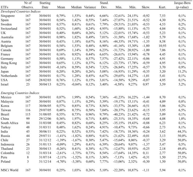
Table 4: Descriptive Statistics for monthly ETFs equity indexes returns, for the out-of-sample period.
Note: the out-of-sample period goes from each variable’s starting date until February 27th 2015. The out-of-sample starting date was then obtained subtracting a window of 60 months to the full period initial date.
The cross analysis of results with MSCI data and EFTs is limited by some methodological difficulties. Among others we would emphasize the different nature of variable construction, but especially distinctive time frame adopted in each case, or still the number of countries in each regional segment. However, although this unavoidable bias we still found a common trend between MSCI sample and EFTs out-of-sample,
ETFs
Nr of Observs.
Starting
Date Mean Median Variance Stand.
Dev. Min. Máx. Skew. Kurt.
Jarque-Bera (p-value)
Developed Countries Indices
Singapore 167 30/04/01 0,79% 1,53% 0,44% 6,66% -32,61% 24,15% -0,92 7,53 0,1% Spain 167 30/04/01 0,54% 1,42% 0,55% 7,44% -27,07% 21,51% -0,52 4,30 0,3% Sweden 167 30/04/01 0,57% 0,81% 0,61% 7,79% -29,51% 21,03% -0,53 4,53 0,2% Switzerland 167 30/04/01 0,52% 1,60% 0,24% 4,95% -15,80% 11,13% -0,73 4,04 0,2% UK 167 30/04/01 0,40% 0,68% 0,26% 5,12% -22,01% 15,74% -0,53 5,23 0,1% Australia 167 30/04/01 0,98% 1,82% 0,49% 7,01% -31,50% 17,68% -1,02 5,79 0,1% Austria 167 30/04/01 0,43% 1,18% 0,67% 8,16% -44,33% 19,71% -1,35 8,58 0,1% Belgium 167 30/04/01 0,54% 1,53% 0,48% 6,90% -41,16% 15,30% -1,80 10,93 0,1% Canada 167 30/04/01 0,69% 1,14% 0,39% 6,23% -31,72% 20,92% -1,00 7,06 0,1% France 167 30/04/01 0,16% 0,92% 0,44% 6,65% -26,61% 15,94% -0,78 4,45 0,1% Germany 167 30/04/01 0,50% 1,13% 0,57% 7,57% -27,42% 22,11% -0,86 4,91 0,1% Hong Kong 167 30/04/01 0,65% 1,12% 0,37% 6,12% -23,73% 17,78% -0,59 4,95 0,1% Italy 167 30/04/01 -0,16% 0,59% 0,54% 7,32% -26,84% 17,25% -0,57 3,70 0,9% Japan 167 30/04/01 0,20% 0,20% 0,26% 5,08% -16,93% 11,29% -0,35 3,20 11,2% Netherlands 167 30/04/01 0,17% 1,28% 0,45% 6,67% -29,65% 14,27% -1,01 5,41 0,1% USA 145 28/02/03 0,76% 1,12% 0,15% 3,81% -14,58% 9,29% -0,87 4,95 0,1% Israel 23 30/04/13 0,23% -0,84% 0,12% 3,40% -4,58% 9,27% 0,97 3,59 5,2%
Emerging Countries Indices
Mexico 167 30/04/01 0,87% 1,99% 0,54% 7,36% -41,23% 16,22% -1,44 8,70 0,1% Malaysia 167 30/04/01 0,87% 1,15% 0,29% 5,39% -19,17% 15,11% -0,41 4,09 0,8% Korea 117 30/06/05 0,57% 0,85% 0,73% 8,56% -33,57% 26,66% -0,51 5,06 0,2% Taiwan 116 29/07/05 0,48% 0,75% 0,50% 7,04% -20,37% 23,62% -0,15 3,95 6,5% Brazil 115 31/08/05 0,55% 0,73% 0,96% 9,79% -40,23% 21,42% -0,72 5,09 0,1% China 99 29/12/06 0,36% 1,97% 0,71% 8,40% -25,31% 18,35% -0,68 4,08 1,0% South Africa 84 31/03/08 0,45% 0,82% 0,68% 8,25% -35,15% 19,43% -0,88 6,23 0,1% Turkey 48 31/03/11 0,48% 1,62% 0,24% 4,91% -10,47% 9,73% -0,66 2,73 8,1% India 45 30/06/11 0,22% 0,52% 0,55% 7,42% -18,73% 18,36% -0,24 3,62 44,3% Russia 44 29/07/11 -1,41% -1,82% 0,88% 9,41% -21,62% 22,49% -0,01 3,13 50,0% Chile 27 31/12/12 -1,39% -1,67% 0,30% 5,47% -15,64% 8,06% -0,37 3,29 50,0% Indonesia 26 31/01/13 -0,09% 1,29% 0,41% 6,39% -20,64% 9,07% -1,37 5,47 0,5% Thailand 23 30/04/13 -0,26% 0,41% 0,38% 6,17% -12,67% 10,93% -0,25 2,18 49,4% Colombia 12 31/03/14 -2,61% -1,73% 0,73% 8,54% -17,64% 14,35% 0,11 2,77 50,0% Peru 8 31/07/14 -2,11% -1,52% 0,11% 3,36% -7,13% 1,42% -0,31 1,50 27,5% Poland 3 31/12/14 -4,70% -3,38% 0,60% 7,77% -13,06% 2,32% -0,30 1,50 50,0%
where developed markets suggest on average better returns than emerging markets, contrarily to what we would from the literature. A plausible explanation could be that out-of-sample ETFs have a too short number of observations in some countries and are close to the 2008 financial crisis in world markets.
4.2 Dynamic Conditional Correlations
At this point in the paper we proceed to investigate a possible worldwide tendency for more integrated markets (emerging and developed), looking at markets’ time-varying correlations. Lower correlations suggest less integrated markets (emerging vs developed). On the other hand, superior correlations imply a closer performance among markets, which decreases investor’s incentive for risk dispersion.
We use the Dynamic Conditional Correlation (DCC) model developed by Engle (2002), to investigate the movement of correlations of stock market indices between Developed and Emerging Markets over the last 15 years. For this purpose we initially plot the dynamic conditional correlations between the MSCI Developed Markets Index and four emerging regional MSCI indices, so that we can have an overall view on the correlation evolution within markets. Then we proceed with a more detailed analysis of the time-varying correlations between the MSCI Developed Markets and sixteen Emerging Countries from Asia (figs. 2,3,4), Europe (figs. 5,6), Middle East and Africa (fig. 7), and South America (figs. 8,9). 5
5
Emerging Regional Markets
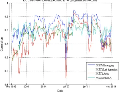
In a preliminary analysis we access the current correlation levels between developed markets and the three emerging regions under consideration on this study. It is clear from the diagrams that significant variations in the correlation structure occurred within the sample period. It can be seen that until 2004 Asian returns show the lower correlation with developed markets, while Latin America and EMEA had similar correlation levels. However, after 2004 the correlation of emerging Asia has grown above the other emerging regions, with exception of a particular day in October 2007 where it suffered the sharpest decrease. This decay didn’t last too long, since emerging regions quickly recovered to the previous high correlation levels. Furthermore, we see from figure 1 that all the emerging regions seem to reach their highest correlation levels during the 2008 crisis period.
Figure 1: Dynamic Conditional Correlation between the MSCI Developed Markets Equity Index returns and the MSCI regional Equity Indexes returns (Emerging; Emerging Latin America; Emerging Asia; Emerging EMEA)
larger integration6 of emerging markets with developed markets. We also reckon a growing correlation between emerging markets and developed markets over time that should be separated from the dramatic events of 2008. The world financial crises apparently gave a major contribution to a general disruption in returns observed.
To better understand the correlation behavior in each region we should embark in a more detailed analysis on a country based correlation with developed markets in the sample.
Emerging Asian Countries
Focusing first on countries belonging to emerging Asian economies, it can be seen that China and Korea are those exhibiting the highest correlation over time. India (figure 2), exhibits the sharpest increase from 1999-2001, coming closer to the Taiwan’s correlation levels afterwards. Indonesia, Malaysia and Thailand (figure 3) do not show such high conditional correlations, however they have also suffered an increase of the correlation with developed markets until 2009. From this group Malaysia presents the most constant increase. Finally Philippines’ correlation with developed markets (figure 4) assumes values between 0,4 and 0,6 having a much lower correlation when compared to Korea. It is interesting to notice that for all the considered Asian countries, the correlations became significantly higher throughout 2008-2009 and persisted at the
6
higher levels, before declining at the end of 2009.
Figure 2: Dynamic Conditional Correlation between the returns of the MSCi Developed Markets Equity Index, and MSCi China, India, Taiwan Equity Indexes returns
Figure 4: Dynamic Conditional Correlation between the returns of the MSCi Developed Markets Equity Index, and MSCi Korea, Philippines Equity Indexes returns
Emerging European Middle East and African (EMEA) countries
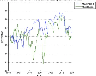
Relatively to emerging European and Middle East countries we find that Poland shows the highest correlation with developed markets over time (Fig. 6). Greece and Hungary had a gradual increase of the correlation over time with developed markets until 2009 (Fig. 5). All the five emerging European countries being considered exhibit a correlation decrease since 2012.
Figure 5: Dynamic Conditional Correlation between the returns of the MSCi Developed Markets Equity Index, and MSCi Czech Republic, Greece, Hungary Equity Indexes returns
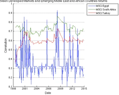
Figure 7: Dynamic Conditional Correlation between the returns of the MSCi Developed Markets Equity Index, and five MSCi Egypt, South Africa and Turkey Equity Indexes returns
Emerging South American Countries
Looking to the correlation of South American emerging economies with the developed markets, it can be seen that Mexico (fig. 8) has the highest correlation over time but also the sharpest decrease around 2007, lowering its correlation level from 0,8 to 0,5.
Figure 8: Dynamic Conditional Correlation between the returns of the MSCi Developed Markets Equity Index, and MSCi Chile, Mexico and Brazil Equity Indexes returns
In sum, from our results it is not clear a general trend in the correlations of asset returns across markets. In general terms we can notice a wide spread positive correlations with developed countries, among the emerging markets studied. However, this inference comes with the perception that there is not a common tendency in emerging markets, with occasional dramatic variations in correlations. Perhaps, the only clear exception should be European emerging markets (Greece; Hungary and Czeck Republic) where a curve in the graph over time allow us to infer a fast marginal gains in correlations with developed countries until 2009, after which the marginal gains came close to zero. Accordingly, we believe that for these countries we should assume a bigger integration with developed countries over time, decreasing as such the opportunity to spread risk by investors. In complementary research to this paper, we would investigate whether these European countries should be instead considered more like a developed market, rather than an emerging market.
Additionally we need to isolate the exogenous effect of the 2008 sub-prime financial crisis, because it is believed that financial crisis of such magnitude could in the short-term provide an environment for fast alignment of world markets generating an undesirable bias.
In order to provide an informational discussion to control the impact of the financial crisis, next we conduct a further analysis specifically about the events around 2008 crisis.
before-crisis. Moreover, the correlations from the period that incorporates the global financial crisis of 2008 are higher when compared to the complete sample.
Table 13: Summary of unconditional correlations for the regional MSCI’ indices
Note: The left side of the table represents the correlations calculated from the complete sample, for the period going from 29 of January 1999 to 21 of November 2014. The entries on the right side of the table represent the correlations for the period before the crisis (on the top); for the period during the crisis (on the middle); for the period after-crisis (the ones below). The period (1) before after-crisis spans from February 1999 to October 2007; the period (2) of crisis spans from November 2007 to December 2010; the period (3) after crisis spans from 2011 to November 2014. All the data is in U.S. dollars and refers to monthly returns.7
This last analysis raises the issue whether the apparent increase of the time-varying
7
these three diferente scenarios, under which we analyze the correlations, were determined taking Valls Pereira et al. (2013) as reference.
Full sample Periods before, during and after the crisis
Emerging Lt. AmericaAsia EMEA Developed World Emerging Lt. AmericaAsia EMEA Developed World
Emerging 1 1
Lt. America 0,918 1 0,886 1
0,956 0,933
Asia 0,953 0,791 1 0,926 0,704 1
0,981 0,892 0,973 0,846
EMEA 0,916 0,853 0,784 1 0,865 0,780 0,662 1
0,966 0,932 0,913 0,925 0,877 0,839
Developed 0,862 0,814 0,786 0,836 1 0,813 0,792 0,690 0,756 1 0,937 0,895 0,909 0,933 0,844 0,791 0,794 0,842
correlations might have been solely driven by the global financial crisis, questioning if markets are in fact more integrated. Given this, we continue this study with a non-dynamic approach, which allows us to examine if in fact emerging countries are already as integrated as developed countries.
4.3 Pairwise Correlations
In this section we intend to study the degree of association within all global stock markets in our sample for the period going from January 1999 to November 2014. Running correlations within the general sample, among every county, we generate a correlation matrix that provides a possible existence of clusters of countries with higher correlation, differentiating those from the rest of the sample. As such, like previously, we assume where higher degrees of correlation are found (closer to 1), larger integration of markets exist, diminishing the gain for risk dispersion.
Looking first to the correlations between emerging countries, based on MSCI indexes, values range from 0,25 to 0,79 (see table 14.1 in appendix). Czech Republic, Greece and Turkey, with values of correlation going from 0,25 to 0,35, reveal the lowest correlation coefficients with the other emerging countries. The countries with higher correlation, over 0,7, are those more close geographically, as it would be expected since they are influenced by the risk of their neighbor countries. This is the case for Poland with Hungary, for example, with a correlation of 0,79. There are more six pairs of countries with correlations coefficients above 0,7.
0,25, while an orange color scale represents the higher values. Values of correlation equal to one are represented on the diagonal matrix with a brown color. So, from the pseudocolor matrix created, we may see that the predominant correlation values that take place between emerging countries are with correlations values going from 0,25 to 0,5, represented by a blue scale. In what refers to the correlations of the emerging countries with the developed markets index, there are twelve countries, out of twenty-one, with values between 0,7 and 0,84, being Brazil the one with the highest value from this group. (See table 14.1 in appendix).
Table 14: Heat color map of the cross-country correlations between 21 MSCI Emerging Countries indices and 5 MSCI regional indices
Note: this table is a matlab output that provides a pseudocolor plot of table 14.1 in appendix
[Insert Table 14.1 here]
From table 15.1 (in appendix) we can get complementary information on the correlations among 21 MSCI Emerging Countries indices with 23 MSCI Developed
Europe, Middle East & Africa MSCi Region Indices
Per Chi Col Me Br Ch In Ido Ko Mal Ph Tw Th CR Egy Gr Hun Pol Rus AS Tur LA Asi EMEADev Em
Per Chi Col Me Br Ch In Ido Ko Mal Ph Tw Th CR Egy Gr Hun Pol Rus AS Tur LA Asi EMEA Dev Em legend 0,25 1 Am e ri ca s A si a EM EA MSC
i R
e
g.
Countries indices. It can be seen that developed countries have higher correlations among them (mostly above 0,7), when compared to the correlations between emerging countries. When analyzing correlations between pairs of emerging with developed countries indices, these tend to range from 0,4 and 0,6. However some emerging countries reveal correlations above 0,7 with several developed countries, being the case of Mexico, Brazil, Korea, Greece, Hungary, Poland and South Africa. Table 15 allows for an overall overview on the correlations between emerging and developed countries. It can be clearly seen that developed countries have higher correlations between them, represented by orange and yellow cells, than with emerging countries, mainly represented by blue cells.
Table 15: Heat color map of the cross-country correlations between 21 MSCI
Emerging Countries indices and 23 MSCI Developed Countries
Note: this table is a matlab output that provides a pseudocolor plot of table 15.1 in appendix
[Insert Table 15.1 here]
In conclusion, correlation matrices do report high correlations among developed countries, and between the emerging regional indices with the developed markets index.
legend
0,23 1
EM
EA
D
e
ve
lo
p
e
d
0M
ar
ke
ts0
M
SC
i0In
d
.
Asia EMEA Developed0Markets0MSCi0indices Americas
Am
e
r.
A
si
However, when compared to developed markets, emerging equity returns aren’t yet reaching the same correlation levels among them and, with the developed equity returns.8 Thus, emerging countries integration is still weak among them, and among these countries and countries with developed markets. Concluding, these results lead us to believe that there might still be potential benefits from diversification in developing markets due to their weak market integration when compared to develop economies.
4.4 Mean-variance model
We provide next a different approach, to the analysis we conducted in the previous section. Although, the above mentioned markets correlation analysis provides an overall picture of the historical performance of individual international markets it is not provided enough information on how returns and risks must be considered in combination. With the MSCI database collected, we essay if in a standard mean variance framework, the set of emerging assets adds substantial diversification benefits by shifting the mean-variance frontier. As the results suggest (fig. 10), the inclusion of emerging market assets in a mean-variance efficient portfolio still contribute to the reduction of the portfolio’s volatility and the increase of expected returns. The blue curve is based on 23 MSCI developed country indices. The red curve reflects the consequence of adding 21 emerging country indices to the problem.
8
All coefficients have been tested for significance (at the 1% level) and most have been
Figure 10 – Mean Variance Efficient Frontier for 21 Emerging Countries and 23 Developed Countries Equity Indices, January 29, 1999 to November 21, 2014
4.5 International ETFs Portfolios
So far we have been using MSCI data to study the performance of global equity markets and examine if there is evidence that it might still be interesting for the investor to invest in emerging markets stocks. However, in order to access if in fact investors may still expect to achieve superior gains by investing in developing countries we propose a different approach using a new dataset. We employ two different asset allocation strategies, to answer a final research question. Is it still possible to obtain a risk reduction, with no compromise of return, assuming a regional dispersion of investment spreading across developed and emerging markets?
equity ETFs. The two portfolios were computed according to the risk parity and the equally weighted out-of-sample asset-allocation strategy. Since the ETFs indices have different sample periods they are added to the portfolios when they get available. Table 4 allows for a better comprehension of all the indices being allocated to both portfolios. Looking first to the sharpe ratio results, on table 7, it can be seen that the portfolios with developed and emerging markets data outperform the ones with only developed markets ETFs, for both asset allocation strategies. In what refers to the performance measures Modified Sharpe Ratio (MSR) and Maximum Drawdown the results also favor the portfolio with emerging markets data.The analysis of the MSR comes relevant since the assets being considered don’t follow a normal statistical distribution, and the standard Sharpe ratio is not sensitive to skewness and kurtosis. When looking only at the Sharpe ratio one can be underestimating potential big losses. However, when looking to the Sortino ratio results these are negative, don’t favoring international diversification in both cases. Also, when comparing the two different asset-allocation strategies the results confirm what is argued in theory, the risk parity strategy leads to better results over the equally weighted one. Relatively to the portfolio’s risk measures, both portfolios’ returns have a negatively skewed distribution. This metric, known as a measure of “pain”, is showing that the returns’ distributions are not symmetrical, having a long tail on its left side, translated into many small gains with a few extreme losses.