FUNDAÇÃO GETÚLIO VARGAS
ESCOLA DE ECONOMIA DE EMPRESAS DE SÃO PAULO
STEFANO TOTO
DINAMICITY AND UNPREDICTABILITY OF EMERGING MARKETS: AN IMPLEMENTATION OF GOETZAMNN AND JORION (1999)
FUNDAÇÃO GETÚLIO VARGAS
ESCOLA DE ECONOMIA DE EMPRESAS DE SÃO PAULO
STEFANO TOTO
DINAMICITY AND UNPREDICTABILITY OF EMERGING MARKETS: AN IMPLEMENTATION OF GOETZAMNN AND JORION (1999)
SÃO PAULO 2015
Dissertação apresentada à Escola de Economia de Empresas de São Paulo da Fundação Getúlio Vargas, como requisito para obtenção do título de Mestre Profissional em Economia.
Campo do Conhecimento:
International Professional Master in Finance
Toto Stefano .DINAMICITY AND UNPREDICTABILITY OF EMERGING MARKETS: AN IMPLEMENTATION OF GOETZAMNN AND JORION (1999) / Stefano Toto. - 2015. 47 f.
Orientador: João Filipe B. V. de Mendonça Mergulhão. Dissertação (mestrado profissional) - Escola de Economia de São Paulo.
1. Mercados emergentes. 2. Risco (Economia). 3. Finanças – Modelos matemáticos. 4. Análise de séries temporais. I. Mergulhão, João Filipe B. V. de Mendonça. II. Dissertação (mestrado profissional) - Escola de Economia de São Paulo. III. Título.
STEFANO TOTO
DINAMICITY AND UNPREDICTABILITY OF EMERGING MARKETS: AN IMPLEMENTATION OF GOETZAMNN AND JORION (1999)
Dissertação apresentada à Escola de Economia de Empresas de São Paulo da Fundação Getúlio Vargas, como requisito para obtenção do título de Mestre Profissional em Economia.
Campo do Conhecimento:
International Professional Master in Finance
Data de Aprovação: ___/___/____.
Banca Examinadora:
______________________________ ___
Prof. Dr. João Filipe B. V. de Mendonça Mergulhão
______________________________ ___
Prof. Dr. João Manuel Gonçalves Amaro de Matos
______________________________ ___
RESUMO
Esta pesquisa é uma implementação de Goetzmann e Jorion (1999 ). De forma a proporcionar um cenário mais realista, foi implementada uma abordagem Garch (1,1) para os resíduos dos retornos e um modelo multifatorial para replicar melhor o risco sistemático de um mercado . As novas simulações revelam novos aspectos dos retornos esperados em mercados emergentes: a imprevisibilidade dos retornos em mercados emergentes com o fator global não dependem do ano de emergência e o risco não sistemático explica os retornos dos mercados emergentes por um período de tempo muito superior. Os
resultados também revelam o impacto elevado da taxa de câmbio, índice de mercadorias e do fator global no retorno esperado em mercados emergentes.
ABSTRACT
This research is to be considered as an implementation of Goetzmann and Jorion (1999). In order to provide a more realistic scenario, we have implemented a Garch (1,1) approach for the residuals of returns and a multifactor model thus to better replicate the systematic risk of a market. The new simulations reveal some new aspects of emerging markets’ expected returns: the unpredictability of the emerging markets’ returns with the global factor does not depend on the year of emergence and that the unsystematic risk explains the returns of emerging markets for a much larger period of time. The results also reveal the high impact of Exchange rate, Commodities index and of the Global factor in emerging markets’ expected return.
TABLE OF CONTENTS 1. Introduction 2. Literature review
3. Goetzman and Jorion model 4. First implementation
Introduction
Emerging markets have been attracting investors since the last century. Markets that were unknown and not considered as a source of investment, have now become attractive due to their very rapid growth. Countries in the Middle East illustrate this idea, as well as Asian countries such as China or Malaysia, that have attracted a lot of investors in the last years. The history of these markets in general is difficult to analyse due to the scarcity of historical data over a long period of time. This happens namely because of events that have caused the close of financial markets in the past (e.g. wars, crisis among other factors) or simply because some of such markets were simply inexistent before.
Many researchers, such as Shiller (1989) Harvey (1994), Brown, Goetzmann and Ross (1995), Goetzman and Jorion (1999), tried to overcome the problem of lack of data, developing techniques that allow to simulate the performance of financial markets. In this study, we extend the model introduced by Goetzmann and Jorion (to be referred as GJ hereafter), by considering a more complex structure of the returns’ residuals and of the systematic risk.
behaviours: some emerge, some sub-emerge, re-emerge again, some markets that never emerge and some other markets that are always considered emerging. A period of one hundred years gives us the possibility to study markets that emerged at any moment of our hypothetical centenary. The systematic, unsystematic risks and the predictability of emerging markets are shown to depend on the year of emergence. The structural changes introduce in their model will prove useful to get additional insights on this behaviour.
In their original paper GJ simulated 100 different markets for a period of one hundred years. The markets were simulated against a single factor model, while the systematic and unsystematic risks were assumed to be Normally distributed. The low correlation between the returns of emerging markets and the returns on a factor that reflects the global market return encouraged investment in emerging economies in the last years. The movement, often unpredictable, of these markets can be a way of introducing portfolio diversification due to their properties in terms of residual risk. Also, the more recent an emerging market is, the higher its systematic risk will be. The high variance of these markets is however compensated by higher expected returns.
To provide a more realistic scenario, we implement a GARCH (1,1) approach for the residuals of returns in order to create a model where the volatility may depend on the period of time. This contrasts with the GJ’s simulation where the residuals series of the markets were Normally distributed.
out, global markets do not empirically satisfy the assumptions of integration and high correlation, and a single factor model does not seem likely to be a good explanation for the market equity return and in particular, for the study of the emerging markets.
The goal of this paper can thus be seen as to improve GJ’s understanding of emerging markets’ behaviour referring to the year of emergence, by using a more realistic structure of the statistical model for the returns.
1.Literature review
The topic of this research has been the object of numerous papers since the end of 20th century. Researchers like Shiller (1989) and Harvey (1994) investigated the survival of the markets and they were the first to use long-term series for the study.
In 1995, Brown, Goetzmann and Ross published a paper entitled “Survival” and the model built could be considered as the starting-point model of our studies. From this point on the model by Brown, Goetzmann and Ross will be referred as BGR.
In BGR the authors specified a model with a series of markets that all started at the same time. The markets were defined by the logarithm of the price p giving the following expression
1) ��=���+ ���1
The markets’ series were assumed to be distributed at intervals [0,T] with µ and σ
constant parameters and z the Brownian path. The markets were assumed to all start at
the same time t and the markets that felled outside of a determined threshold “survived
series” were taken into consideration for the studies.
The most interesting aspect of BGR's results is the positive bias imparted onto the mean.
For small σ2, this bias tends to !!
(! ! !)! 2. Thus, there is a functional relationship between the bias and the variance of the markets’ series. The more volatile the markets are, the higher is the probability of failing, and thus these markets have a larger bias in the mean.
Another characteristic which emerged from BGR’s study is the correlation between the year of emergence of a market and the average return for the emerging equity markets; BGR found that average return in the first years after the emergence is higher than average near the end of time period3
In 1999, GJ presented the paper “Re- emerging market”. This paper could be seen as an implementation of BGR and as the basic model for our implementations.
In GJ the researchers considered a time series of 100 years and simulated 100 markets for 2500 times with a single factor model. The main difference from the earlier paper was the year of emergence of the markets, which was considered random in the time series.
2
Stephen J. Brown, William N. Goetzmann, Stphen A. Ross.1995. “Survival”. The Journal of Finance, Vol.3.
3 Stephen J. Brown, William N. Goetzmann, Stphen A. Ross.1995. “Survival”. The
2.Goetzman and Jorion model
In GJ the model used for the simulation of market expected returns is a single factor
model described by the formula below
2) Ri = αi + βiRm + ei
where:
1. E(ei) = 0 ∀i = 1, 2, . . . , n
2. E (ei (Rm – E (Rm))) = 0 ∀i = 1, 2, . . . , n
3. E (eiej) = 0 ∀i, j = 1, 2, . . , n
This model divides returns into two components – a unique part, αi
– a market-related part, βi.RM..
β measures the sensitivity of the markets’ returns to the global factor movements ,
while αi represents the abnormal return of the global factor over the theoretical
expected return of the markets.
The Ri represents the expected markets’ returns and the ei the residual risk.
The risk of a market includes a systematic risk and an unsystematic one. Systematic risk refers to the risk, which is common to all markets determined by the betas in the model. Unsystematic risk is the risk associated with the individual market determined by the residual risk.4
4
Simulation process:
The simulations of the indexes are constructed under the following conditions:
1. Rmj is simulated using i.i.d. Normal returns with an annual mean of 10% and an
annual standard deviation of 20%
2. eis simulated with i.i.d. which draws from a normal distribution with a mean of zero and a random standard deviation drawn from a uniform distribution between 10% and 30%.
3.βkis the constant loading on the global market index and is drawn randomly from a uniform distribution between zero and two.
4. α is set to zero.
Markets begin randomly with starting dates drawn from a uniform distribution over the interval t= 1 to t = 99.
2500 simulations for 100 markets are made. What is common for every simulation of each market is the value of Rm, while the values of the other variables are randomly
distributed in the way described above. The goal is to obtain markets that differ in terms of expected return and risk.
There are two important assumptions: no dividend payments and no mispricing in any of the markets, so Rm, is constant through out.
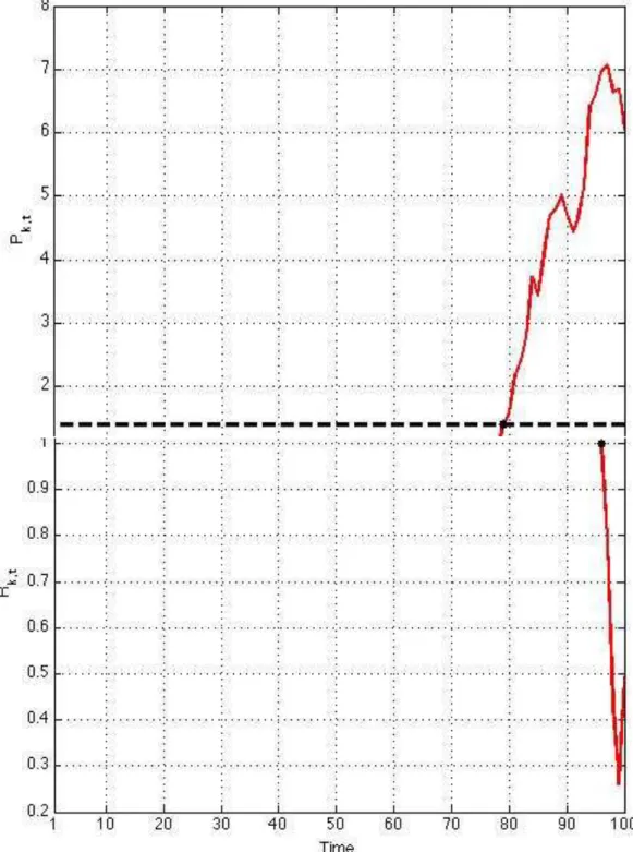
Only the markets that exceed a barrier called threshold, (defined by the formula Pk,t=Pk,0 + standard deviation of each market) in their last movements are observed.
The initial market price, �!,!, is assumed equal to one and all markets are assumed to
start at one standard deviation of �! below the capitalization threshold. Fig.1 shows one
market that was studied.
The market in figure 1 is a typical market that was taken into consideration by GJ: it is defined as an emergent market, because it has crossed the barrier in an upwards direction and in particular because its last crossing was due to growth.
Contrary, Figure 2 shows a kind of market that never emerged so GJ do not consider for the results’ analysis.
For each simulation five variables were saved: t1 (the year when the market started,
which, as previously stated, is completely random), te (the year of the last emergence),
Rm (the market return), Rk,t (the return of the specific country) and βk to obtain Bias. GJ
used all 2500 *100 (numbers of the markets) simulations to obtain the results.
Considering only the last time period of markets’ emergence, reserve particular interest the difference between the mean annual return of the survive series and the true beta times the global market return.
GJ defined as “ Bias” in the mean annual return the difference described below:
3) ����� =[ !
!!!! �!,! ! !!!!!! ]−��[ ! !!!! �!,! ! !!!!!! ]
Where �� is the true market beta. R-squareis defined equal to:
4) R2=!"#(!) !"#(!)
Where
• Var(r) = β2Var(Rm)
• Var(R) = β2Var(Rm) + Var(ε).
information provided by the start date of the series in relation to the emergence date of the series.
GJ offers some new results regarding the analysis presented in BGR. The results can be divided into sorting effects and survival effects; the sorting effects are the most
innovative part of GJ’s work.
The survival effects come from the analysis on the bias as defined in equation (1). GJ evidenced the correlation between the year of emergence of a market and bias. The graph (Appendix figure 1) represents the quantiles distribution for the bias and it shows the positive correlation between the bias and the residuals. For two markets emerging at the same time the one with higher residuals risk has a higher bias. This positive correlation between the bias and residuals can be seen as a positive correlation between the expected return and the part of variance not explained by the global factor.
The sorting effects on the surviving markets come from the study on the betas and the R-square with the emergence. Figure 2 in Appendix shows the quartiles distribution for the betas and the figure underlines a higher betas value for markets that emerged early in the time series than for the markets that emerged later. The observation on the betas reflected the fact that the earlier is the emergence of a market higher is the unconditional expected return.
R-square than worldwide factors. Moreover, it is one of the reasons why emerging markets are used for the portfolio diversification.
3.First implementation
The first implementation as stated above will be concerned with the unsystematic risk of the GJ model. In order to create a model where the volatility may be depending on the period of time, we simulated the residual risk with a GARCH (1,1). The other assumptions of the GJ model will be maintained. The simulation process and the analysis of the results comply with GJ.
The aim of our improvement was to have a more realistic prospective of the residual series’ behavior and to track the variations in the volatility over time.5 Indeed in a GARCH (1,1) the next period forecast of variance is a blend of the last period forecast and the last period’s squared return6 as it is illustrated in the next model resume.
The resume of the model is7:
5) Rit =α+ βrmt +Yt
Yt = αt
5
Luc BauwensSébastien Laurentand Jeroen V. K. Rombouts, 2006.” Multivariate GARCH models: a survey” Journal of financial econometrics
6
Robert F. Engle, Sergio M. Focardi and Frank J. Fabozzi, “Arch/Garch Models in Applied Financial Econometrics “
7Tim BOLLERSLEV,1986.”Generalized Autoregressive Conditional
where
αt=εtσt with εt ~N(0,1),
σ2t=Ε[Yt2 | Yt-1] = ω+ �!εt−1+�!σ2t−1
σ2t =ω+ �
!ε 2
t−1+�!σ2t−1
and • ω≥0 • 0 >�
!+�!<1
which are the usual restrictions of GARCH models ensuring covariance stationary. The �
! value is a measure of the conditional variance sensitivity in relation to shock of the market; a high �
! means that the volatility is very sensitive to market’ shock. �
! is an indicator of the persistence of the conditional volatility with respect to market
shock. If �
! is high the shock of the market is long lasting. ω and �!+�! are the estimators of the long-term volatility of the model.
When !
(!!!!!) is high it means that the long-term volatility is high as well.
To find the three parameters w, �
!, �!, a GARCH(1,1) model was simulated for the
S&P 500 index between 2005 and 2009. The fixed value was found to be ω=0.012341;
�
!=0.081; �! =0.91. Moreover A GARCH(1,1) model was simulated with a MSCI World Index obtaining completely different GARCH parameters: ω= 0.00003822; �
!=0.7760; �!=0.1622. The two different scenarios are analysed as two different cases
Results
The first implementation shows differences respect GJ on the bias and R-square quantiles distribution; different is the result on the betas quantiles distribution that is the same of GJ.
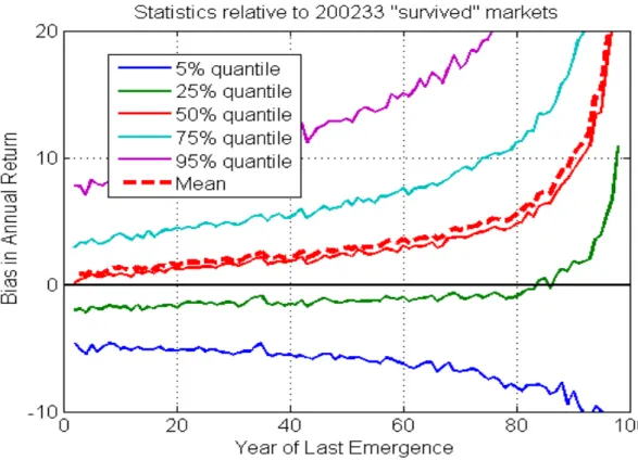
Figure 3 shows the percentile distribution of the bias for the emerging markets obtained with our implementation. It shows that the bias tends to zero for markets that emerged in the first part of our hypothetical century while tends to 20 for the market that emerged in the last decade of the century.
The main difference with GJ (Appendix 1 ) regards the steepness of the curves in the percentile distribution.
In GJ results the bias has a high value only for the markets that emerged recently and it is close to zero for the markets that emerged between years 0 and 80; our analysis reveals a different scenario indeed the increase of bias is more gradual. Markets that emerged in year 40 present a bias close to 5 and the value tends to increase for markets that emerged more recently, up to 20 for the markets that emerged in the last decade. The simulations reveal a more dynamic model underlining the strong correlation between the year of emergence of a market and the residual series represented by the bias.
Figure 3: The percentile Bias distribution obtained with the implementation to GJ’s model.
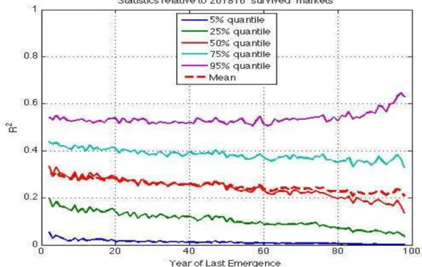
Figure 4 shows the percentile distribution of the residual risk for the survival markets. In GJ the average R-square mean starts for the markets that emerged in the year zero with a value of 0.6 while the values go down for the markets that emerged later, arriving at a value of 0.5 for the markets that emerged only in the last decade.
As far as the implementation is concerned we have a very different result. Indeed the start value of R-square is around 0.3 and the final value, i.e. for markets that emerged in the year 100, is around 0,22
results; the only thing that changes is the portion of variance explained, which is 30% for markets that emerged early, and 20% for newly emerged markets.
Figure 4: The percentile R-square distribution with the implementation on the GJ’s model.
The strong correlation between emerging markets and unsystematic risk is confirmed also by the results on R-square.
Another relevant aspect that emerges from the implementation is that we will never have markets with 100% of variance explained. The best scenario is 60 % at 95 percentile and this happens just for markets that emerged in the first years of the century. This result differs from what GJ obtained.
In GJ 60 % of variance explained corresponded to the R-square mean for the older survivals. Moreover for a very small number of cases the variance explained by the model is 90 %.
The empirical result behind this is the reason that emerging markets are sold to implement portfolio diversification.
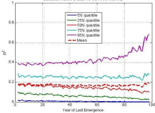
In order to better understand the correlation of the R-square with the year of emergence of a market we used different indexes to find the GARCH model parameters.
An interesting result was reserving using the MSCI World index between 2000 and 2014.
Figure 5 shows the percentile distribution with the new parameters and what is interesting to notice that the mean of explained variance is constant for all the emerging markets irrespective of the emergency. The R-square for markets that emerged in the first part of the century is lower than the pervious scenario and it is equals to 20%. The result confirms the dynamicity and unpredictability of emerging markets.
4.Second implementation
The second implementation deals with the systematic risk of the GJ’ model.
In GJ the authors simulated 100 markets’ returns with a single factor model whereas in this section we present the same study done in GJ for the country price formation but using a multi-factorial model and basing the estimation of the simulation parameters on real markets data. The goal is to achieve a deeper and more accurate analysis of the correlation between year of emergence of a market and the systematic risk than GJ made.
As predictors in the changes of markets’ return five factors were selected: Oil price, commodities index, Currency risk, World index and the dividend yield8.
The emerging equity market is influenced by numerous factors that can be divided into internal or external influencers. Some events are unpredictable like political incidents, wars etc., others are predictable and they depend on macro or microeconomic events. The paper will concentrate on the five factors that are considered to be the most important and likely to have the greatest influence with regard to the emergence of a market by Geert Bekaert (1993) and Campbell (1995).
In Campbell, the analysis is concentrated between 1980 and 1992 whereas this paper will concern the period 2000 until 2014. Campbell analysed the relationship between the emerging markets and five factors (the world market equity return, the return on
8 Campbell R.Harvey in,1995,”The Risk Exposure of Emerging Equity Markets “ The
foreign currency index, a change in the price of oil, growth in world industrial production, and world inflation rate). Campbell’s main result was that in the final years the correlation between the factors and the markets was higher. One reason could have been world integration 9. Based on Campbell’s result, this study takes into consideration three of the five factors analysed by Campbell (1995) (world market equity index, currency risk, and oil price) plus two others factor that were used by Geert Bekaert (1993) dividend yield and commodity risk. 10 The choice behind a restricted number of factors, five, rests on the analysis of Campbell (1995).
The scope of this paper is to capture with the five variables three economic forces: commodity prices, exchange prices and the world global risk.
Assuming that the markets’ returns are influenced by just five factors we can divide the five selected variables of the present study into local instruments and global instruments. Indeed three of the five factors are the same for all the countries and two are specific and different for each country.
The country-specific variables are the dividend yield and the exchange rate. The first of these is the dividend yield inherent of the index of every individual country, the second is the exchange rate for each country against the dollar.
The reason behind the exchange rate choice is that the continuing increases in world trade and capital movements have made the exchange rates one of the main
9
“Campbell R. Harvey ,1995”The risk exposure of emerging equity markets”. The world bank Economic review. Vol.9 No1
10
determinants of business profitability and equity prices11. Exchange rate changes directly influence the international competitiveness of firms, given their impact on input and output price 12. Basically, foreign exchange rate volatility influences the value of the markets equity since the future cash flows of the firms change with the fluctuations in the foreign exchange rates.“
Dividend yield is selected in relation to its good characteristic as a proxy for the long- term expected excess return, as Campbell and Ammer (1993) affirmed. 13
The common-factor variables, contrarily, are the same in terms of values for all the forty countries and they are selected in order to summarise the factors that have the biggest influence in the world on emerging markets, commodities and oil, plus a factor that could summarize the connection with the global world, the world index.
Data description
Data on forty countries are taken from the MSCI market index. The forty countries are divided between developed and emerging countries. Eighteen of the forty markets are
11
Kim, K. (2003). Dollar Exchange Rate and Stock Price: Evidence from Multivariate Cointegration and Error Correction model. Review of Financial Economics, 12, 301-313.
12
Joseph, N. (2002). Modelling the impacts of interest rate and exchange rate changes on UK Stock Returns. Derivatives Use, Trading & Regulation, 7(4), 306-323.
13
The mean returns of the countries indexes and of the five factors in each country
The table lists the mean returns for the five factors returns in each country and for the forty indexes returns between 2000 and 2014
Index Oil Commodity
Index MSCI World Index Exchange rate Dividend Yield OCDE Markets
Australia 0.0011 0.0014 0.0006 0.0003 0.0003 40876
Austria 0.0002 0.0014 0.0006 0.0003 0.0009 25960
Belgium 0.0001 0.0014 0.0006 0.0003 0.0009 34912
Canada 0.0010 0.0014 0.0006 0.0003 -0.0003 21747
Denmark 0.0017 0.0014 0.0006 0.0003 -0.0002 16379
Finland -0.0009 0.0014 0.0006 0.0003 0.0009 35881
France 0.0001 0.0014 0.0006 0.0003 0.0009 29938
Denmark 0.0002 0.0014 0.0006 0.0003 0.0009 28146
Hong kong 0.0007 0.0014 0.0006 0.0003 -0.0000 34358
ireland -0.0009 0.0014 0.0006 0.0003 0.0009 26482
Israel 0.0006 0.0014 0.0006 0.0003 -0.0001 22086
Italy -0.0006 0.0014 0.0006 0.0003 0.0009 38894
Japan -0.0003 0.0014 0.0006 0.0003 0.0002 15146
Netherlands 0.0001 0.0014 0.0006 0.0003 0.0009 32877
New Zealand 0.0006 0.0014 0.0006 0.0003 -0.0005 50115
Norway 0.0009 0.0014 0.0006 0.0003 -0.0001 34968
Portugal -0.0010 0.0014 0.0006 0.0003 0.0009 41712
Singapore 0.0005 0.0014 0.0006 0.0003 -0.0003 35486
Spain 0.0003 0.0014 0.0006 0.0003 0.0009 39331
Sweden 0.0005 0.0014 0.0006 0.0003 -0.0001 29807
Switzerland 0.0009 0.0014 0.0006 0.0003 -0.0006 23312
United 0.0000 0.0014 0.0006 0.0003 0.0001 23312
Usa 0.0004 0.0014 0.0006 0.0003 0 18615
Emerging Markets
Brazil 0.0011 0.0014 0.0006 0.0003 0.0004 30394
Chile 0.0010 0.0014 0.0006 0.0003 0.0002 25511
China 0.0008 0.0014 0.0006 0.0003 -0.0004 24756
Colombia 0.0031 0.0014 0.0006 0.0003 0.0003 33578
Czech 0.0019 0.0014 0.0006 0.0003 -0.0006 46147
Greece -0.0028 0.0014 0.0006 0.0003 0.0009 33853
Hungary 0.0002 0.0014 0.0006 0.0003 0.0000 21321
India 0.0015 0.0014 0.0006 0.0003 0.0004 14391
Indonesia 0.0012 0.0014 0.0006 0.0003 -0.0000 16321
Korea 0.0010 0.0014 0.0006 0.0003 -0.0001 32656
Malasyia 0.0016 0.0014 0.0006 0.0003 0.0005 17474
Mexico 0.0026 0.0014 0.0006 0.0003 -0.0002 33778
Peru 0.0010 0.0014 0.0006 0.0003 0.0001 24933
Philippines 0.0005 0.0014 0.0006 0.0003 -0.0002 27014
Poland 0.0010 0.0014 0.0006 0.0003 0.0008 19085
South Africa 0.0013 0.0014 0.0006 0.0003 0.0008 31516
Thailand 0.0015 0.0014 0.0006 0.0003 -0.0002 31384
Model description
The next step of the paper is to study the movements of 40 casual markets in relation to the five factors and a threshold that represents the line of emergence of a market, with the same process used by GJ. In order to reach GJ’s methodology we compute a previous study on real market data and we base the assumption for the simulation on this study results.
Using the data of the indexes of forty countries between 2000 and 2014 (see table 1 for the full list of countries)as a dependent variable and the values of the dividend yield, the returns of commodity index, oil price, world index and exchange rate as independent ones, forty regressions were conducted.
The model of the regression is presented below.
3) Ri = αi + �!�!+�!�!+�!�!+�!�!+�!�!+ ei
where:
– R! represents the return of oil
– R! represents the return of the commodity index
– R! represents the MSCI World Index
– R! represents the return on the exchange rate
– R! represents the dividend yield
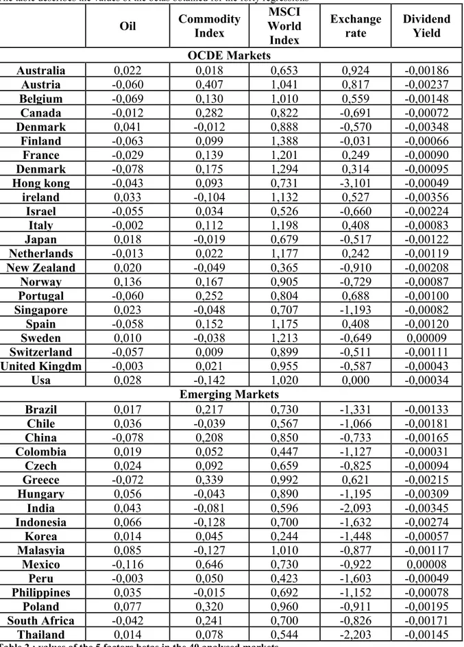
BETAS VALUES OF REGRESSION
The table describes the values of the betas obtained for the forty regressions
Oil Commodity
Index MSCI World Index Exchange rate Dividend Yield OCDE Markets
Australia 0,022 0,018 0,653 0,924 -0,00186
Austria -0,060 0,407 1,041 0,817 -0,00237
Belgium -0,069 0,130 1,010 0,559 -0,00148
Canada -0,012 0,282 0,822 -0,691 -0,00072
Denmark 0,041 -0,012 0,888 -0,570 -0,00348
Finland -0,063 0,099 1,388 -0,031 -0,00066
France -0,029 0,139 1,201 0,249 -0,00090
Denmark -0,078 0,175 1,294 0,314 -0,00095
Hong kong -0,043 0,093 0,731 -3,101 -0,00049
ireland 0,033 -0,104 1,132 0,527 -0,00356
Israel -0,055 0,034 0,526 -0,660 -0,00224
Italy -0,002 0,112 1,198 0,408 -0,00083
Japan 0,018 -0,019 0,679 -0,517 -0,00122
Netherlands -0,013 0,022 1,177 0,242 -0,00119
New Zealand 0,020 -0,049 0,365 -0,910 -0,00208
Norway 0,136 0,167 0,905 -0,729 -0,00087
Portugal -0,060 0,252 0,804 0,688 -0,00100
Singapore 0,023 -0,048 0,707 -1,193 -0,00082
Spain -0,058 0,152 1,175 0,408 -0,00120
Sweden 0,010 -0,038 1,213 -0,649 0,00009
Switzerland -0,057 0,009 0,899 -0,511 -0,00111
United Kingdm -0,003 0,021 0,955 -0,587 -0,00043
Usa 0,028 -0,142 1,020 0,000 -0,00034
Emerging Markets
Brazil 0,017 0,217 0,730 -1,331 -0,00133
Chile 0,036 -0,039 0,567 -1,066 -0,00181
China -0,078 0,208 0,850 -0,733 -0,00165
Colombia 0,019 0,052 0,447 -1,127 -0,00031
Czech Republic
0,024 0,092 0,659 -0,825 -0,00094
Greece -0,072 0,339 0,992 0,621 -0,00215
Hungary 0,056 -0,043 0,890 -1,195 -0,00309
India 0,043 -0,081 0,596 -2,093 -0,00345
Indonesia 0,066 -0,128 0,700 -1,632 -0,00274
Korea 0,014 0,045 0,244 -1,448 -0,00057
Malasyia 0,085 -0,127 1,010 -0,877 -0,00117
Mexico -0,116 0,646 0,730 -0,922 0,00008
Peru -0,003 0,050 0,423 -1,603 -0,00049
Philippines 0,035 -0,015 0,692 -1,152 -0,00078
Poland 0,077 0,320 0,960 -0,911 -0,00195
South Africa -0,042 0,241 0,700 -0,826 -0,00171
Thailand 0,014 0,078 0,544 -2,203 -0,00145
The model we use for the simulations of the forty markets is equal to:
�!,! = �!,!�!,!+�!,!
where:
– �!,! is the market expected return
– �!,! is a vector of five beta factors. Each beta is a simulation of the betas used in
the regression. The beta values for the simulations are randomly drawn between the beta minimum and beta maximum of each specific beta value obtained trough the forty regressions.(table 3)
MAXIMUM AND MINIMUM BETAS
The table describes the maximum and minimum values for each beta
obtained trough the forty regressions
Beta max Betas Min
Oil 0,135 -0,115
Commodity 0,645 -0,142
MSCI World
Index 1,388 0,2431
Exchange rate 0,924 -3,100
Dividend Yield 9,32E-05 -0,0036
Table 3 : Values max and min of each betas
1. �!,! is a matrix of random value that replicate the five factors used in the
copula distribution for the market factors regards the objective of taking into account the correlation between the five factors used as risk factors.
– �!,! is the residual risk of the series. It is simulated with a Normal distribution
with mean zero and standard deviation equal to the standard deviation of the forty markets’ residual series obtained by the regression.
The use of copulas to model different risks has become common in financial markets, in particular, in this study it is used because the distribution of the returns on
an index will depend not only on the univariate distributions of the individual risk factors and but also on the dependence between each of the factors14.
For a five-factor model the most appropriate univariate distribution for each dependent variable could be chosen and the factors simulated separately. The problem is that, by doing this, the interdependencies between all the variables would not be taken into account. One way to consider the correlation is to use a copula. The relation between the factors would then be represented by a multivariate probability distribution function, which is informative on the joint outcomes of the variables.15
14 “ Copula-Based Models for Financial Time SeriesFirst version”: 31 August 2006.
This version: 19 November 2007. Andrew J. Patton Department of Economics and Oxford-Man Institute of Quantitative Finance, University of Oxford, Manor Road, Oxford OX1 3UQ, United Kingdom.
15 Svetlozar T., Rachev. Stein, Michael. Sun, Wei. 2009. “Copula Concepts in
Financial Markets”
Results
In order to obtain a valid number of results the 40 markets simulations were run 3000 times. The same process as in GJ is used to define an emerged and sub- emerged market. A threshold is defined as equal to ��!+��� (��!) and the markets that go beyond the line in their last movement are taken into consideration and they are considered as emerging markets.
The analysis was focused on the relation between betas and emergence.
The results of the five betas are presented in figures 6 to 10. Unlike GJ model, here, we can notice that there is no relation between the betas and the year of emergence of the market but what is relevant is the different influence of the five risk factors on the emergence of the market.
The percentile distributions present different pictures on the values of the betas compared to GJ.
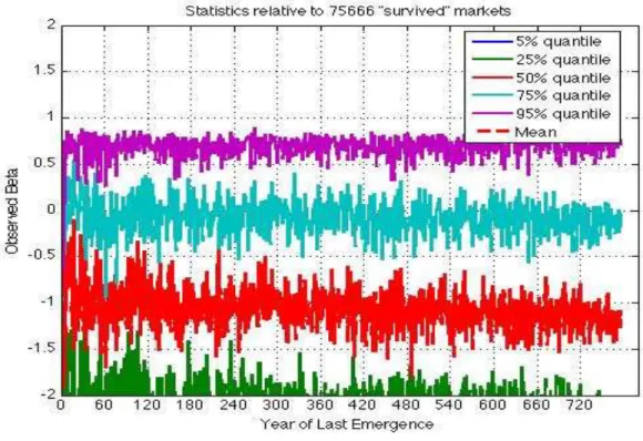
Figure 6: The exchange rate beta distribution results due to the implementations on the GJ’s model.
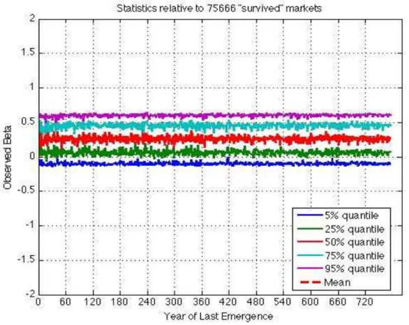
The second most influential factor is the World Index with a mean of 0,7 (figure 7).
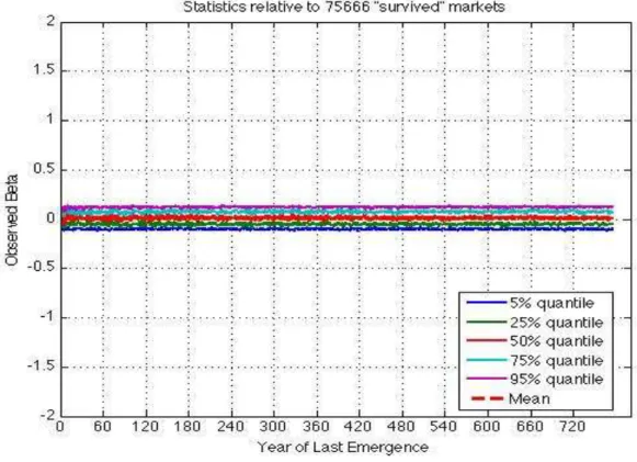
Figure 8 shows the percentile distribution of the commodity returns. It has a mean of 0,3, lower than World index and exchange rate, however it has a positive impact on the markets emergence.
Figure 8: the commodity index beta quantiles distribution results due to the implementations on the GJ’s model.
Figure 9: The oil beta distribution results due to the implementations on the GJ’s model.
One interesting aspect that arises from the analysis on the real data is that the values of the betas seem not to depend on the year of emergence of a market and this contrasts with the results found in GJ
The results on the bias have the same GJ’ outcomes indeed the two percentile distributions have the same trend; the mean is equal to 20 for markets that emerged in the last years of the century while is equals to zero for all the others emerged market
5.Conclusion
The results described in this paper show that returns on emerging markets are dynamic, unpredictable and very connected with the unsystematic risk. This seems to be so much truer, the more recently they have emerged. As compared to GJ’s results, our analysis confirms and enriches what they have found. The two technical improvements of this paper allow to conclude that emerging markets are more aggressive and unpredictable than GJ’s results suggested.
in the GARCH (1,1) model the correlation of emerging markets’ returns with the global factor does not depend on the year of emergence, as opposed to what GJ’s result would suggest. This implies that emergent markets performances are less predictable than imagined.
The second technical improvement of the model was to explain the systematic risk through a multifactor model as opposed to GJ’s single factor approach. Following the literature five explanatory factors were considered, among which the exchange rate was shown to be the most influential factor in the emergence of a market. The systematic risk of the emerging market aggregates the contribution of the five different factors. As the exchange rate is the one providing larger variability (variance) in the past twenty years, its weight in the aggregate result is the more significant. The results also reveal the high impact of the Commodities index and of the Global factor in emerging markets’ expected return. In contrast, Oil index and dividend yields have a relatively low influence on the systematic risk of emerging markets.
References:
• Svetlozar T., Rachev. Stein, Michael. Sun, Wei. 2009. “Copula Concepts in Financial Markets”
• Nieto, Belèn. 2001. “ Evaluating multi-beta pricing models: an empirical analysis with spanish market data”. “Revista de Economia Financeira, article N.4 (pag 80-109)
• Luc Bauwens Sébastien Laurent and Jeroen V. K. Rombouts, 2006.”
Multivariate GARCH models: a survey”. Journal of Financial Econometrics. • Bekaert,Geert.1995. “Market Integration and Investment Barriers in Emerging
Equity Markets”. The world Bank Economic Review, Vol.9 (pag 75-107)
• Stephen J. Brown, William N. Goetzmann, Stphen A. Ross.1995. “Survival”. The Journal of Finance, Vol.3.
• Patton, J.Andrew.2007. “Copula-Based Models for Financial Time Series” • Edwin J. Elton and Martin J. Gruber. 1988. “ A Multi Index Risk Model Of the
Japanese Stock Market”. Japan and the World Economy, Vol.1 (21-44)
• Thomas G. Stephan, Raimond Maurer, Martin Durr. “ A multiple Factor Modeal For European Stocks”
• Renata Bonfiglio, Paolo Guderzo. 2000. “Un Modello Econometrico
Multifattoriale Dell’Indice Consob Generale Della Borsa di Milano”. Greta, Vol.8.
• Richard Roll, Stephen A. Ross. 1980. “An Empirical Investigation of the Arbitrage Pricing Theory”. The Journal of Finance, Vol.5,N
• William N. Goetzmann ,Pjilippe Jorion. 1999. “Re- emerging markets”
Integration of Stock Markets in Latin America”. Journal of Economic Integration.
• Blair Henry, Peter.2000.”Stock Market Liberalization, Economic Reform,and Emerging Market Equity Prices. The Journal of Finance,Vol.LV,No2.
• Rouwenehorst, K.Geert.1997. “Local return and turnover in emerging stock markets”.
• Bekaert Geert,Erb Claude B.,Harvey Campbell R. and Viskanta Tadas E.. 1998.”Distributional Characteristics of Emerging Market Returns and Asset Allocation”.
• Bekaert Geert, Harvey Campbell R.” Emerging Equity Market Volatility”
• Harvey, Campbell R. 1995.”Predictable Risk and Returns in Emerging Markets”.The Review of Financial Studies,Vol.8 No3
• Harvey, Campbell R. 1995. “The Risk Exposure of Emerging Markets”. The
World Bank Economic Review,Vol.9 No.1
• Bekaert Geert, Harvey Campbell R..”Time-Varying World Market Integration” • Andersen, T. Bollerslev, T., Diebold, F.X. and Labys, P. (2001), "The
Distribution of Realized Exchange Rate Volatility," Journal of the American Statistical Association, 96, 42-55.
• Fama Eugene F., French Kenneth R.1996.”Multifactor Explanations of Asset Pricing Anomalies”. The Journal of Finance,Vol.11,No1
• Agrawal Gaurav,Srivastav Aniruddh Kumar,Srivastava Ankita.2010.”A study of Exchange Rates Movement and Stock market Volatility”.International Journal of Business and Management,Vol.5 No12
• Modigliani Franco and Pogue Gerald A. 1973. “An introduction to Risk and
Return Concepts and Evidence.
• Campbell R.Harvey, 1993,"The Risk and Predictability of International Equity Returns" Review of Financial Studies 6, 527-566
• Shiller, Robert J., 1989, “Market volatility” (MIT Press, Cambridge, Mass.).
• Tim BOLLERSLEV,1986.”Generalized Autoregressive Conditional
Heteroskedasticity”. Journal of Econometrics 31 (pages (307-327)).
• www.bloomberg.com
• www.investopedia.com
• www.wikipedia.com
Appendixes:
Appendix 1: The Bias quantiles distribution in GJ
Appendix 3 R-square quantiles distribution in GJ.
Appendix 4 Betas distribution in first implementation model (Garch(1,1) with S&P).
Appendix 5 R square distribution in GARCH MODEL with World Index
Appendix 6 R-square distribution for the multifactor implementation
Appendix 8 : an example of market obtained in the simulations.