Repositório Institucional UFC: Integration and hedging efficiency between brazilian and u.s. ethanol markets

(1)

INTEGRAÇÃO E EFICIÊNCIA DO HEDGE NOS MERCADOS DE

ETANOL DO BRASIL E EUA

INTEGRACIÓN Y EFICIENCIA DE HEDGE EN LOS MERCADOS

DE ETANOL DE BRASIL Y ESTADOS UNIDOS

Daniel Henrique Dario Capitani

Assistant Professor, School of Applied Sciences, University of Campinas (FCA/UNICAMP), Limeira-SP, Brazil.

daniel.capitani@fca.unicamp.br

José César Cruz Junior

Assistant Professor, Department of Economics, Federal University of São Carlos (Ufscar), Sorocaba-SP, Brazil cesarcruz@ufscar.br

Julyerme Matheus Tonin

Assistant Professor, Department of Economics, State University of Maringa (UEM), Maringá-PR, Brazil jmtonin@uem.br

Contextus ISSNe 2178-9258 Organização: Comitê Científico Interinstitucional Editor Científico: Diego de Queiroz Machado Avaliação: double blind review pelo SEER/OJS Edição de texto e de layout: Carlos Daniel Andrade Recebido em 17/08/2017 Aceito em 11/03/2018 2ª versão aceita em 11/04/2018

ABSTRACT

This study proposes to assess the ethanol market integration between U.S. and Brazil focusing on the investigation of the existence of an international ethanol price reference. We estimate a structural vector autoregressive model with error correction (SVEC) while considering not only ethanol sugar and corn prices in Brazil and in the U.S. but also international oil prices. Then we examine simultaneous hedging strategies by considering domestic and foreign futures contracts positions in the CME, NYMEX, and BM&FBOVESPA futures exchanges. Our results highlight a weak integration between U.S. and Brazil ethanol markets, as well as low levels of hedge effectiveness in using foreign ethanol futures contracts, which suggests the absence of a price reference in the global market.

Keywords: Market integration. Time series modelling. Hedge effectiveness. Ethanol.

RESUMO

Este trabalho visa avaliar o grau de integração nos mercados de etanol dos EUA e Brasil, investigando a existência de um preço como referência internacional que possa servir de base aos agentes dessa cadeia produtiva. Foi estimado um modelo autorregressivo vetorial estrutural com correção de erros (SVEC), considerando tanto os preços de etanol, milho e açúcar, no Brasil e nos Estados Unidos, quanto o preço internacional do petróleo. Posteriormente, foram examinadas eficiências de estratégias simultâneas de hedge considerando operações com os contratos futuros de etanol na CME, NYMEX e BM&FBOVESPA. Em geral, os resultados indicam que tais mercados possuem baixo grau de integração, respondendo majoritariamente a variáveis domésticas. Além disso, evidencia-se uma baixa eficiência na operação de hedge cruzado com contratos futuros de etanol em outras bolsas, sugerindo, portanto, uma baixa integração dos preços no mercado internacional.

Palavras-chave: Integração de mercado. Modelos de séries temporais. Efetividade do hedge. Etanol.

RESUMEN

(2)

NYMEX y BM&FBOVESPA. Los resultados indican que estos mercados tienen una baja integración, respondiendo mayoritariamente a variables domésticas. Además, se evidencia una eficiencia reducida en la operación de cobertura cruzada con los contratos futuros de etanol en otras bolsas, sugiriendo, por lo tanto, una baja integración de los precios en el mercado internacional.

Palabras-clave: Integración de mercado; Modelos de series temporales; Efectividad de cobertura; Etanol.

1 INTRODUCTION

The growing importance of energy supply and the new environmental policies created to reduce greenhouse gas (GHG) emissions have introduced relevant issues in the applied agricultural economics literature. Biofuels markets, in particular ethanol, have stimulated important debates where Brazil and the U.S. play important roles, since they are the largest world producers (EPA, 2016).

The development and the importance of the ethanol production in Brazil and in the U.S. have emerged in different periods, and for different reasons. In Brazil, the sugarcane-based ethanol production started in the 1970s aiming to reduce the dependence from international oil prices. More recently, the ethanol production in the country has been driven by the dominant flex-fuel vehicle fleet, and by the market regulation that imposes a mandate to blend anhydrous ethanol with gasoline. In the U.S., the corn-based ethanol production was consolidated only after federal mandates determined a minimum production of anhydrous ethanol in the country. The development and availability

of technologies that enable the flexible uses of agricultural commodities contribute partly to raise global-market volatility, creating new price drives for these markets (BORRAS et al., 2016).

(3)

RAPSOMANIKIS, 2008; DABRIK et al., 2016; RODRIGUES; BACCHI, 2016).

Market participants who face price risk should consider all the aforementioned differences between local and international markets when creating their marketing strategies, since they contribute to increasing market volatility, and can determine different price patterns in each market (BORRAS et al., 2016). Aiming to create different market strategies, market participants can use the derivative markets to promote hedging opportunities, to discover prices, and to promote financial stability to their economies (LIEN; ZHANG, 2008; SAXENA; VILLAR, 2008). Even though derivatives markets can contribute to a more efficient hedging strategy in markets with low trading volume and liquidity, individual bids and asks can influence prices and bring more risk to the market. Markets with those characteristics are referred to as thin markets (ADJEMIAN; SAITONE; SEXTON, 2016), such as the ethanol futures markets in Brazil and in the U.S. The investigation of how the spot and futures markets in both countries are integrated is particularly relevant for those who use derivatives as risk management tools. Intuitively, the less integrated the markets, the lower the hedging efficiency. Therefore, the research questions we try to answer with this study

are: Is there a reference market for ethanol prices that can guide hedging strategies? Are hedging strategies efficient in the Brazilian and U.S. ethanol markets? We try to answer these questions by using local prices from relevant spot markets in both countries, and futures prices from three futures exchanges.

Our main purposes are: (i) to investigate whether Brazilian and U.S. prices are cointegrated, by assessing their short and long-run relationships as well as causality effects simulated by shocks; and (ii) to identify which is the most efficient futures contract in reducing price risk for different hedging strategies.

Our methodological approach includes Johansen cointegration analysis and the estimation of a Structural Vector Auto-Regressive Model with errors correction (SVEC). We also analyze impulse-response functions, as suggested by Sims (1986) and Bernanke (1986). We test for hedging efficiency by estimating minimum variance hedge ratios based on the model developed by Nayak and Turvey (2000), which accounts for hedging in using the ethanol and exchange rate futures contracts simultaneously.

(4)

international reference prices for feedstock or substitute goods. Therefore, we estimate an autoregressive model that also includes domestic sugar and corn prices, and international oil prices to assess the determinants of ethanol prices. Balcombe and Rapsomanikis (2008) and Kristoufek (2016) used similar procedures in their analysis but different econometric models. The dataset covers the period from January 2010 to December 2016. For the hedging efficiency analysis, we use daily ethanol cash prices in both countries, and ethanol futures prices from three different futures exchanges (CME, NYMEX and BMFBOVESPA), for the same period (2010-2016). We also use the exchange rate BRL/USD in the simultaneous hedge model.

Our primary hypothesis is that several recent events in the American and Brazilian markets (crop seasonality, harvest shortfall, government intervention, etc.) have guided their domestic price dynamics individually. The need to execute the federal mandate and the establishment of a new industry in the U.S. have brought about a fast ethanol production increase. In addition, adverse weather events such as the 2012 drought in the U.S. Midwest affected domestic corn production and stocks, influencing ethanol local prices and imports. In Brazil, the recent federal

government intervention in gasoline prices limited ethanol production expansion by reducing the industry margins. In addition, climate effects in South Brazil had affected sugarcane yield negatively and reduced ethanol supply. All the aforementioned events combined can explain the low connection between the Brazilian and the U.S. markets and may affect international price dynamics, as well as the efficiency of hedging with ethanol futures contracts.

2 ETHANOL MARKET

INTEGRATION

Brazil—the world’s largest

sugarcane producer—is a traditional producer and consumer of biofuels, mostly ethanol derived from sugarcane. In addition, ethanol consumption have intensified after the introduction of flex-fuel vehicles in 2003, since that biofuel works as a close substitute for gasoline. On the supply side, the decisions regarding ethanol production are made by considering the domestic sugarcane and international sugar prices as well as traded volumes. The gasoline and oil prices also influence the fluctuations of ethanol prices and production in the country.

(5)

biofuel producer in the world, sharing with Brazil a significant part of international ethanol production. Besides, the U.S. production is mostly intended for blending with gasoline in low volume, varying from 5% to 15%. The implication of the large anhydrous ethanol production is the close linkage with fuel markets. Consequently, variations in gasoline, oil and other fossil fuel prices can directly affect ethanol prices and production.

Only few studies have recently explored price and volatility transmission of biofuels in the international market level. Indeed, several studies were developed in the past years to study the dynamics of biofuel prices and their linkages to feedstock and fuel prices. Yet, despite the importance of the U.S. and Brazil in the biofuel international market, most recent studies focused their analysis only on domestic price dynamics.

Balcombe and Rapsomanikis (2008) investigated the long-term connection between ethanol, sugar and oil prices in Brazil. Their findings indicate the importance of oil prices’ determining ethanol and sugar prices, as well as the causality effect from sugar prices to domestic ethanol prices. The authors suggest that biofuels do not seem to have any significant impact on commodity prices in the Brazilian market.

Other studies also assessed the long-run relationship between ethanol, sugar, sugarcane and gasoline prices in Brazil. Bentivolgio et al. (2016) explored the influences of Brazilian ethanol prices on sugar and gasoline prices by using Granger causality tests in addition to a VECM model. Their study found evidence that ethanol prices have no effect on sugar or gasoline prices. However, in the same study they found gasoline prices to drive ethanol prices in Brazil, in the short and long-run.

Chen and Saghaian (2015) investigated price linkages among Brazilian ethanol and sugar prices to international oil prices by harnessing data between 2003 and 2014. First, their study tested for structural break points to determine the period when the three commodities’ prices established a common linkage. Later, by using a cointegration test and a VEC model estimation, they could not find a long-run relationship between prices. In addition, sugar prices drive more ethanol prices than the opposite, while oil prices were not relevant to explain sugar or ethanol prices.

(6)

findings indicated not only a greater influence of gasoline on oil and ethanol prices but also the absence of a long-run relationship among fuel (gasoline, oil, and ethanol) and grain (soybeans and corn) prices.

Serra et al. (2011) used a VECM to evaluate the connections of corn, ethanol, gasoline and oil prices in the U.S., during the period of 2000-2008. Differently from other studies, they found prices were cointegrated. Specifically, their results suggest that ethanol prices were guided by variations on gasoline and corn prices. Merkusheva and Rapsonamanikis (2014) analyzed price linkages among ethanol, oil, and other grains in the U.S. market, indicating that oil prices guide all others. However, they suggest a different interpretation to the short-run analysis between fuel and grain markets, i.e., they did not find evidence that prices had a causality effect on each other.

Other previous studies used time series models to estimate linkages among ethanol, fuels, and commodity prices, focusing especially on the impacts of biofuels on commodity prices. Serra et al. (2013) structured an extensive literature review, exploring different methodology approaches. The authors concluded that both partial equilibrium and time series models have been used in the literature to

investigate biofuel prices relationship with fossil fuels and other agricultural commodities and have obtained similar results. Similarly, Tyner (2010) explored the links between energy and agricultural markets since the boom of commodity prices in the U.S. The authors highlighted the possible association of the corn ethanol industry increase with the establishment of federal mandates to the ethanol production.

(7)

prices in their analysis. Their results suggest a strong causality relation of gasoline prices to ethanol prices. They also found a linkage between feedstock and ethanol prices but in different ways, once ethanol production increases with an increase in sugar prices in Brazil. In the U.S., on the other hand, a rise in corn prices causes reduction on ethanol production.

Considering the relative small number of studies related to the investigation of price linkages in the ethanol international market, this research aims to present new evidence to the discussion on this topic. First, with the analysis of the domestic causality effects of ethanol, feedstock and oil prices. Second, by evaluating ethanol market integration between the U.S. and Brazil. Finally, including new elements to the analysis of hedging effectiveness of using futures contracts in both countries.

3 RESEARCH METHOD

We divide our empirical analysis into three different steps. First, we evaluate the regional dynamics of ethanol prices by testing for prices’ cointegration and causality effects in the U.S. and Brazilian domestic markets. Second, we investigate

ethanol prices’ integration between the Brazilian and the U.S. markets. At last, we investigate the hedge effectiveness of ethanol futures contracts, in different futures exchanges.

3.1 Market integration methodological approach

We use traditional time series approaches to identify market integration between spot and future markets in Brazil and in the U.S. A cointegration test is used to identify the presence of a long-run relationship among prices (integration), and the vector error correction model (VECM) is used to verify how prices adjust from deviations to the equilibrium in the short run.

If all prices in the model are non-stationary and have the same integration order, then we test the existence of a long-run relationship among prices by using the well-known Johansen multivariate test. If we find at least one cointegration relationship, then we conclude that markets are indeed integrated. The number of cointegration relationships can be determined after estimating the model in equation 1:

(8)

Where _𝐴₀ is a vector containing the intercept, and _∆𝑃_𝑡 is a (n × 1) vector of the

first difference of prices. The (n × n) matrix Πcan be written as Π = αβ’, where α and β

are (n × r) matrices containing the speed of

adjustment parameters and the cointegrating vectors, respectively. The matrix _Π_𝑖 contains all the parameters estimated to represent the impact of lagged variables in the system, and _𝜀_𝑡 is a vector of random error terms (LUTKEPOHL, 2006).

According to Enders (2005), when the model presented in (1) is estimated by using the maximum likelihood method, the

rank of Π is determined. Two different test

statistics (trace and eigenvalue) are used to

test the null hypothesis of rank Π = 0. If the

null hypothesis cannot be rejected, then prices are not cointegrated and there is no integration among markets. On the other hand, if the null hypothesis is rejected, a sequential test is conducted to determine the number of cointegrating relationships.

Once we find the markets are cointegrated, we can use the matrix Π to

investigate long-run price dynamics and how prices adjust to deviations away from the equilibrium. The Vector Error Correction Model (VECM) can then be used, as it not only allows for estimating the adjustment back to equilibrium but it also allows both for causality testing and for

determining the impact of shocks on different prices by using impulse-response functions.

For this reason, we use the Structural VECM, an alternative decomposition of VECM, which consists of a system of simultaneous equations that enables us to obtain the dependency relationships between variables. Furthermore, this method can provide well-fitted variance decomposition of forecast errors, as well as shock estimations through the impulse-response function from a structured matrix of contemporaneous relations, as proposed by Sims (1986) and Bernanke (1986).

The impulse-response functions provide the forecast of impulse elasticities for k periods ahead. The elasticities

(9)

a particular variable as well as by others (ENDERS, 2005). In addition, the Structural VECM estimation shows the contemporaneous relationship of the variables’ system, which indicates the number of restrictions regarding the

economic theory, and the restriction of maximum number of contemporaneous restrictions (HAMILTON, 1994). The structural VECM consists of a structural VAR with error correction. The SVAR is expressed by the following equation:

𝐵0𝑥𝑡 = 𝐵1 𝑥𝑡−1+ 𝐵2 𝑥𝑡−2+ ⋯ + 𝐵𝑝 𝑥𝑡−𝑝+ u𝑡 (2)

Where xt is the vector of prices in

the system; Bj are the matrices (n x n) for

each j and B0 is the matrix of

contemporaneous relationship; ut is a vector

n x 1 of orthogonal shocks where the

components are not serially correlated.

Furthermore, we implement Granger causality tests by using bivariate vector autoregressions to determine whether lagged information in one specific price set provides any statistically significant information to another price set forecast. If not, we conclude that the first price set does not Granger-cause the second. Once we have the results of all pairwise causality tests, we have a better indication of how markets in Brazil and in the U.S. are related. Therefore, this approach can help to build a more appropriate sequence of shocks when estimating impulse-response functions.

This analysis can provide indications of integration in the ethanol markets in both countries, and reveals how the markets are related in the long and short-run. In addition, the analysis in the regional level can indicate local spot prices interactions.

3.2 Hedge effectiveness

In this section we focus on estimating the optimal hedge ratio, based on the model proposed by Nayak and Turvey (2000). According to this model, a producer sells the commodity in the cash local market, while hedging the commodity price by using a foreign futures contract and simultaneously hedging the exchange rate risk. Using the mean-variance framework, the model can be written as follows:

(10)

Where HR is the hedged revenue; R

is the spot revenue at the end of the period;

h and c are the amounts of contracts traded

on the ethanol and exchange rate futures markets, respectively; F1 e f2 are the ethanol

futures prices at the beginning, and at the end of the period, respectively; E1 e e2 are

the exchange rate futures at the beginning, and at the end of the period, respectively; er

represents the spot exchange rate at the end

of the period; G, M, Q1 e q2 refer to the

positions and prices for the crop yield futures contracts, which are not evaluated in our study.

The primary approach of the income hedging of Nayak and Turvey (2000) implemented the perspective of simultaneous price and exchange rate hedging (HS):

𝑯𝑺 = 𝑹 + 𝒉𝒇𝒆𝒓+ 𝒄𝒆 (4)

Where, for simplification, _{𝑓 = 𝐹}₁_{− 𝑓}₂ and _{𝑒 = 𝐸}₁_{− 𝑒}₂. We can therefore represent the variance of equation (4) as:

𝝈𝑯𝑺𝟐 = 𝝈𝑹𝟐+ 𝒉𝟐𝝈𝒇𝒆𝟐 𝒓+ 𝒄𝟐𝝈𝒆𝟐+ 𝟐𝒉𝝈𝑹,𝒇𝒆𝒓+ 𝟐𝒄𝝈𝑹,𝒆+ 𝟐𝒉𝒄𝝈𝒇𝒆𝒓,𝒆 (5)

Where the variances are given by

𝜎𝑅2 = 𝑉𝑎𝑟(𝑅); 𝜎𝑓𝑒2𝑟 = 𝑉𝑎𝑟(𝑓𝑒𝑟); 𝜎𝑒2 = 𝑉𝑎𝑟(𝑒); and the covariances are _𝜎_{𝑅,𝑓𝑒}_𝑟 ₌

𝐶𝑜𝑣(𝑅, 𝑓𝑒𝑟); 𝜎𝑅,𝑒 = 𝐶𝑜𝑣(𝑅, 𝑒) e 𝜎𝑓𝑒𝑟,𝑒 = 𝐶𝑜𝑣(𝑓𝑒𝑟, 𝑒).

Then, hedging decision is based on the minimum variance of the simultaneous

hedge in relation to the futures price (h) and

the exchange rate (c) positions, resulting in

the first-order conditions:

𝝏𝝈𝑯𝑺𝟐

𝝏𝒉 = 𝟐𝒉𝝈𝒇𝒆𝟐 𝒓+ 𝟐𝝈𝑹,𝒇𝒆𝒓+ 𝟐𝒄𝝈𝒇𝒆𝒓,𝒆 = 𝟎 𝝏𝝈𝑯𝑺𝟐

𝝏𝒄 = 𝟐𝒄𝝈𝒆𝟐+ 𝟐𝝈𝑹,𝒆+ 𝟐𝒉𝝈𝒇𝒆𝒓,𝒆 = 𝟎

(𝟔)

(11)

ℎ∗₌ 1 1−𝜌_{𝑓𝑒𝑟,𝑒}2 (−

𝜎_{𝑅,𝑓𝑒𝑟} 𝜎_𝑓𝑒𝑟2 +

𝜎𝑅,𝑒𝜎𝑓𝑒𝑟,𝑒

𝜎_𝑓𝑒𝑟2 𝜎𝑒2 ) (7.1)

𝒄∗₌ 𝟏 𝟏−𝝆_{𝒇𝒆𝒓,𝒆}𝟐 (−

𝝈𝑹,𝒆 𝝈𝒆𝟐 +

𝝈_{𝑹,𝒇𝒆𝒓}𝝈_{𝒇𝒆𝒓,𝒆}

𝝈_𝒇𝒆𝒓𝟐 𝝈𝒆𝟐 ) (7.2)

Where, h* and c* are respectively the

positions of minimum risk in the price and

the currency futures markets; _𝝆_𝒇𝒆𝟐 _𝒓_,𝒆 ₌

(𝝈𝒇𝒆𝒓,𝒆 𝝈_𝒇𝒆𝒓𝝈𝒆)

𝟐

represents the squared correlation

coefficient between futures prices

(expressed in local currency) and exchange rate futures.

We can use the results of the minimization problem given in equations 7.1 and 7.2 to replace the optimal values in equation 3:

(𝝈𝑯𝑺𝑹𝑴)𝟐= 𝝈𝑹𝟐+ (𝒉∗)𝟐𝝈𝒇𝒆𝟐 𝒓+ (𝒄∗)𝟐𝝈𝒆𝟐+ 𝟐𝒉∗𝝈𝑹,𝒇𝒆𝒓+ 𝟐𝒄∗𝝈𝑹,𝒆+ 𝟐𝒉∗𝒄𝝈𝒇𝒆𝒓,𝒆 (8)

Therefore, the absolute risk reduction is given by the difference between

the non-hedged revenue and the simultaneous hedged revenue.

𝑹𝑹𝑯𝑺= 𝝈𝑹𝟐− (𝝈𝑯𝑺𝑹𝑴)𝟐 =_𝜽𝝈𝟏_𝒆𝟐(

𝝈_{𝑹,𝒇𝒆𝒓}𝝈_{𝒇𝒆𝒓,𝒆} 𝝈_𝒇𝒆𝒓𝟐 − 𝝈𝑹,𝒆)

𝟐

+𝝈𝑹,𝒇𝒆𝒓

𝝈_𝒇𝒆𝒓𝟐 (9.1)

Where _{𝜃 = 1 − 𝜌}_𝑓𝑒2 _𝑟_,𝑒, and the other

variables have already been specified.

We can evaluate the risk reduction obtained with the use of the futures price contracts (only) in the hedged revenue if we

assume that _𝜎_𝑅,𝑒 _{= 0} and_𝜎_𝑓𝑒_𝑟_,𝑒_{= 0}. See

Equation 9.2. Similarly, we can evaluate the risk reduction obtained with the use of exchange rate futures contracts (only) by assuming that _𝜎_{𝑅,𝑓𝑒}_𝑟 _{= 0}e _𝜎_𝑓𝑒_𝑟_,𝑒_{= 0}. See

Equation 9.3.

𝑅𝑅ℎ = −𝜎_𝜎𝑅,𝑓𝑒𝑟

𝑓𝑒𝑟2 (9.2)

𝑹𝑹𝒄= −𝝈_𝝈𝑹,𝒆_𝒆𝟐 (9.3)

Equations 9.1 through 9.3 are the basis for the comparative analysis of three

(12)

hedge exchange rate only using currency futures contracts; iii) the simultaneous hedge using both commodity futures prices and currency futures contracts.

3.3 Data

The first part of the analysis consists of estimating models to investigate ethanol price relationships and the linkage between the U.S. and the Brazilian markets. The dataset consists of daily cash prices for ethanol (USA and Brazil), corn (USA), sugar (Brazil) and oil (brent crude futures) for the period between January 2010 and December 2016. The U.S. cash ethanol and corn prices correspond to the average price in the main producing regions in the Midwest as well as the cash ethanol and sugar prices in Brazil are related to the average price for São Paulo state (largest sugarcane producer in Brazil). Prices for similar commodities are converted to the same units, i.e., corn and sugar are expressed in USD/ton, and ethanol (from both countries) and oil prices in USD/m3_.

We also use the natural log of prices in our analysis.

The second step is the analysis of hedge effectiveness of cash ethanol with ethanol futures contracts in the Brazilian (BMFBovespa) and U.S. exchanges (CME and NYMEX). The cash ethanol prices in

both markets are the same included in the time series models described before. We use the following futures prices in our study: hydrous ethanol (BMFBovespa), ethanol (CME/CBOT), and the Chicago ethanol (Platts) (NYMEX). We use daily prices from January 2010 to December 2016 and roll the nearby contract on the first day of the expiration month. For the simultaneous hedge analysis, we also included the exchange rate futures contract at BMFBovespa (BRL/USD).

Given the low liquidity of BMFBovespa in comparison to the CME and the NYMEX ethanol futures contracts, the simultaneous hedge analysis is restricted to the relationship of cash ethanol prices in Brazil to the CME and NYMEX ethanol futures. Therefore, we do not use the same procedure to analyze simultaneous hedging strategies between U.S. cash ethanol prices and BMFBovespa ethanol futures.

4 RESULTS

(13)

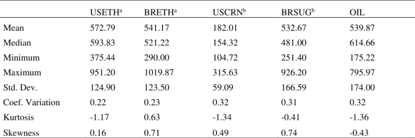
Brazilian sugar) show positive skewness and negative excess of kurtosis, suggesting the presence of asymmetric distribution

with slim tails. Ethanol prices in Brazil show positive skewness and kurtosis, and oil prices negative skewness and kurtosis.

Table 1 – Summary statistics of commodities prices (2010-2016)

USETHa _BRETHa _USCRNb _BRSUGb _OIL

Mean 572.79 541.17 182.01 532.67 539.87

Median 593.83 521.22 154.32 481.00 614.66

Minimum 375.44 290.00 104.72 251.40 175.22

Maximum 951.20 1019.87 315.63 926.20 795.97

Std. Dev. 124.90 123.50 59.09 166.59 174.00

Coef. Variation 0.22 0.23 0.32 0.31 0.32

Kurtosis -1.17 0.63 -1.34 -0.41 -1.36

Skewness 0.16 0.71 0.49 0.74 -0.43

Note: a: US$/m3; b: US$/ton; USETH, BRETH, USCRN, and BRSUG indicate cash prices of U.S. ethanol,

Brazilian ethanol, U.S. corn, Brazilian sugar, respectively, and OIL represents the international futures oil prices

(brent). All prices are deflated by USA Price Consumer Index (December 2016).

During the period of our analysis, ethanol prices in both countries had similar volatility levels (price dispersion). In spite of that, Brazilian traders had their prices fluctuating within a wider range (maximum minus minimum prices) than traders in the U.S. In addition, biofuel prices showed lower volatility than oil prices, especially after 2014, when oil prices became more volatile albeit in lower levels than historical prices series. Ethanol prices follow a similar trend but Brazilian ones seem to have lower levels than those of the U.S. between 2012 and 2015. This pattern is probably a consequence of the federal domestic intervention in gasoline prices, establishing maximum baselines for the ethanol prices variation (Figure 2 – Appendix).

Following our preliminary analysis, we used the augmented Dickey-Fuller (ADF) unit root test to check for stationarity. We found all log-price series were nonstationary. All log-price series were found to be stationary after we ran the same test in the first difference (Table 6 –

Appendix).

(14)

investigate the long-run relationship among the variables, as well as their particular short-run interactions, the VECM was estimated.

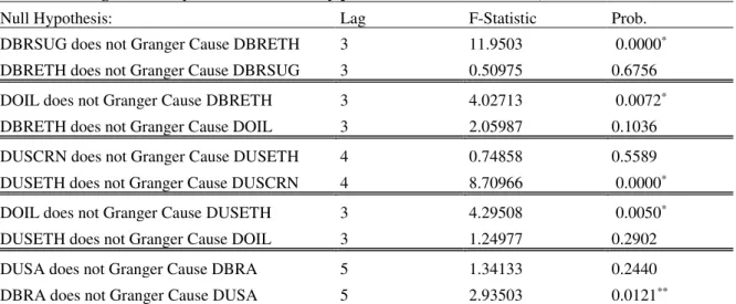
Granger causality tests for each pair of variables were used to identify how domestic prices are related. First, for the U.S. market, causality tests were applied between ethanol-corn prices and ethanol-oil prices. Table 2 shows that ethanol prices cause corn prices, but corn prices do not cause ethanol prices, suggesting that ethanol prices have significant information predicting feedstock prices. This result is not consistent with other studies, but can be explained by the significant raise of the U.S. ethanol production, as well as the dramatic

impact on the corn production (and stocks) after the 2013 drought in the Midwest.

According to the results in Table 2, ethanol prices seem to be caused by oil prices in the U.S. market, indicating that fossil fuel prices are relevant to explain the dynamics of biofuel prices. Similar results were found for the Brazilian market between oil and ethanol prices. In this case, ethanol prices are caused by oil prices. Besides, we found a causality relationship of sugar prices to ethanol prices, which means that the feedstock (substitute goods) are relevant in determining ethanol prices in the Brazilian market. Lastly, the causality test for ethanol prices in both countries exhibited one direction, from the Brazilian ethanol prices to the U.S. ethanol prices.

Table 2 – Granger causality between commodity prices in Brazil and the U.S., 2010-2016

Null Hypothesis: Lag F-Statistic Prob.

DBRSUG does not Granger Cause DBRETH 3 11.9503 0.0000*

DBRETH does not Granger Cause DBRSUG 3 0.50975 0.6756 DOIL does not Granger Cause DBRETH 3 4.02713 0.0072*

DBRETH does not Granger Cause DOIL 3 2.05987 0.1036 DUSCRN does not Granger Cause DUSETH 4 0.74858 0.5589 DUSETH does not Granger Cause DUSCRN 4 8.70966 0.0000*

DOIL does not Granger Cause DUSETH 3 4.29508 0.0050*

DUSETH does not Granger Cause DOIL 3 1.24977 0.2902

DUSA does not Granger Cause DBRA 5 1.34133 0.2440

DBRA does not Granger Cause DUSA 5 2.93503 0.0121** *_{Statistically significant at 1% level;}**_{statistically significant at 5% level.}

Note: DUSETH, DBRETH, DUSCRN, and DBRSUG indicate cash prices in the Δ1st difference of U.S. ethanol,

Brazilian ethanol, U.S. corn, Brazilian sugar, respectively. DOIL is the 1st difference for international futures oil

(15)

We then used a structural VECM to identify the short-run dynamics of prices. Basically, the structure of the SVECM was built by simulating the influence of cash ethanol from Brazil to the U.S. prices, and vice-versa. We also investigated

relationships between corn and sugar prices in the U.S. and in Brazil, as well as the influence of oil prices on domestic ethanol prices. The results are expressed by the variance decomposition analysis shown in Tables 3 and 4.

Table 3 – Decomposition of variance for U.S. ethanol (%)

Step Std Error DUSETH DBRETH DUSCRN DBRSUG DOIL

1 0.006 88.640 4.205 7.153 0.002 0.000

2 0.007 72.090 9.425 10.216 3.382 4.887

3 0.009 57.404 8.049 20.830 5.307 8.410

4 0.009 53.135 8.696 20.443 6.653 11.074

5 0.009 50.020 8.593 19.530 7.802 14.055

6 0.009 48.760 8.490 19.457 8.210 15.084

7 0.009 48.330 8.564 19.306 8.411 15.389

8 0.009 48.175 8.574 19.214 8.514 15.523

9 0.009 48.133 8.576 19.184 8.551 15.555

10 0.009 48.123 8.579 19.175 8.565 15.558

11 0.009 48.124 8.578 19.173 8.569 15.556

12 0.009 48.125 8.578 19.173 8.570 15.554

Average 0.009 54.922 8.242 17.738 6.878 12.220

Note: DUSETH, DBRETH, DUSCRN, and DBRSUGindicate cash prices in the Δ1st difference of U.S. ethanol,

prices (brent).

Table 4 – Decomposition of variance for Brazilian ethanol prices (%)

Week Std Error DUSETH DBRETH DUSCRN DBRSUG DOIL

1 0.012 4.379 95.214 0.353 0.054 0.000

2 0.013 8.344 85.481 0.270 5.894 0.011

3 0.014 7.983 83.344 1.102 6.518 1.053

4 0.014 7.623 80.913 1.063 8.143 2.258

5 0.014 7.458 79.216 1.235 8.742 3.349

6 0.014 7.376 78.463 1.340 9.131 3.691

(16)

(CONTINUATION)

7 0.014 7.380 78.063 1.332 9.320 3.906

8 0.014 7.404 77.823 1.327 9.426 4.020

9 0.014 7.418 77.741 1.326 9.464 4.051

10 0.014 7.435 77.696 1.329 9.481 4.059

11 0.014 7.445 77.677 1.330 9.487 4.061

12 0.014 7.450 77.669 1.332 9.489 4.060

Average 0.014 7.308 80.775 1.112 7.929 2.877

prices (brent).

The variance decomposition of forecast errors for the U.S. ethanol shows evidence of several variables’ influence on prices, i.e., corn and oil prices can explain about 35% of ethanol prices in the U.S., while the Brazilian ethanol and sugar prices influence merely 17% of the U.S. ethanol market. In contrast, the Brazilian ethanol prices are more independent, explaining almost 80% of their own price variation. Sugar prices (7.9%), U.S. ethanol prices

(7.3%) and oil prices (2.9%) exhibited a weaker connection with the Brazilian ethanol prices.

We then used the impulse-response function estimates to investigate ethanol prices behavior after we simulated shocks on each price. The function results are presented in Figure 1.

Figure 1 – Cumulative shocks from the estimated impulse-response functions for commodity prices (%)

-2,0 -1,0 0,0 1,0 2,0

1 2 3 4 5 6 7 8 9 10 11 12

(a) U.S. ethanol

DUSETH DBRETH

DUSCRN DBRSUG

-0,5 0,0 0,5 1,0 1,5 2,0 2,5

1 2 3 4 5 6 7 8 9 10 11 12

(b) Brazilian ethanol

DUSETH DBRETH

(17)

prices (brent).

A positive shock of 1% on corn prices could affect the U.S. ethanol prices for more than one week, increasing the biofuel prices by roughly 0.5%. This result is similar to the cumulative shocks on the own variable (corn prices) that represents a cumulative increase of 0.75% in the price after 12 weeks (Figure 1c). In addition, there is no significant connection between the U.S. corn prices and Brazilian ethanol prices, suggesting that corn prices only influence the U.S. ethanol price.

Conversely, a shock on sugar prices can produce a significant change on ethanol prices in both markets (Brazil and USA). A

simulated shock of 1% on sugar prices in Brazil can result in an increase of sugar prices close to 2.75% in later periods. The result of this shock is also relevant on ethanol prices in Brazil and in the U.S., accounting into a possible rise of 1.15% and 0.77% respectively (Figure 1d). These results are closely related to the Granger causality analysis for ethanol prices in both markets, with the Brazilian ethanol causing U.S. ethanol prices.

Similar results were also found after simulating a 1% shock on Brazilian ethanol prices. As a result, we could expect increases of 0.60% in the U.S. ethanol price,

-0,5 0,0 0,5 1,0 1,5

1 2 3 4 5 6 7 8 9 10 11 12

(c) U.S. corn

DUSETH DBRETH

DUSCRN DBRSUG

-1,0 0,0 1,0 2,0 3,0

1 2 3 4 5 6 7 8 9 10 11 12

(d) Brazilian sugar

DUSETH DBRETH

DUSCRN DBRSUG

-1,0 -0,5 0,0 0,5 1,0 1,5

1 2 3 4 5 6 7 8 9 10 11 12

(e) Oil

DUSETH DBRETH DUSCRN

(18)

of 0.95% in sugar price, and nearly 1.95% in the Brazilian ethanol price, after 12 weeks (Figure 1b). However, according to the impulse-response function analyses, a shock on the U.S. ethanol prices does not seem to cause the expected effect, reducing Brazilian ethanol prices (Figure 1a). In any case, this result must be relativized due to the apparently high influence of domestic policy on the U.S. ethanol prices.

Finally, the response of a 1% shock on oil prices seem to have an opposite effect on commodity prices, showing that prices can decrease over time (Figure 1e). This outcome can be associated to an exogoenous effect of oil prices as direct components of fuels and feedstock prices. The opposite effect on commodity prices can also be related to an impact on commodity production costs as well as to the regulation of fuel markets that can mitigate the impact of prices on local markets.

4.1 Hedging effectiveness

Our hedging effectiveness analysis was based on Nayak and Turvey’s (2000) methodological approach and consists of

two parts. First, we calculated the hedge effectiveness considering a Brazilian hedger trading ethanol futures contracts at each of the three different exchanges at the same time he hedged his currency risk trading currency futures contracts at the BMFBovespa. Second, we analyzed the position of a hedger in the U.S., trading ethanol futures contracts at the CME Group and NYMEX. We analyzed the effectiveness of different hedging strategies for different crop years.

(19)

Table 5 – Results of hedge efficiency for strategies of cash ethanol and futures contracts in the CME Group, NYMEX and BMFBovespa by crop/year

Crop year BR BM&Fa _{BR CME}b _{BR NYMEX}b _{US CME}c _{US NYMEX}c

2010/11 95.06% 80.28% 78.71% 96.51% 97.88%

2011/12 90.52% 42.27% 43.25% 84.03% 92.80%

2012/13 89.41% 22.77% 22.52% 90.36% 90.25%

2013/14 96.08% 20.35% 19.46% 61.46% 71.76%

2014/15 96.26% 28.05% 26.31% 86.23% 89.90%

2015/16 98.06% 57.47% 61.44% 78.08% 79.95%

a: Brazilian hedger using BMFBovespa ethanol futures contracts, only; b: Brazilian hedger using either the CME or the NYMEX ethanol futures contract, with simultaneous currency hedge at the BMFBovespa; c: U.S. hedger using either the CME or the NYMEX ethanol futures contract.

The results for U.S. hedgers using futures contracts either from the CME Group or from NYMEX are similar to the results found for Brazilian hedgers trading only ethanol futures contracts in the Brazilian exchange. In general, the expected hedge effectiveness was higher when using the NYMEX ethanol futures contracts for most of the years, except for 2012/2013.

The low effectiveness for Brazilians using simultaneous hedging strategies may indicate the importance of regional variables in the ethanol price formation, both in the U.S. and in Brazil. In addition, during the most part of the analyzed period, both countries had mandatory policies in their biofuels and fuels markets. The combination of all these factors could influence prices determination according to domestic ethanol, feedstock and fuels supply and demand, which maintain a low connection with biofuels markets, and could explain the weak linkage of ethanol prices

in the international market. Moreover, the high variation of the BRL/USD exchange rate may have influenced the results for Brazilian hedgers trading ethanol futures contracts in the U.S.

5 CONCLUSIONS

This study investigated market integration and hedging efficiency between the world’s two largest ethanol producers: USA and Brazil. Our investigation focused on price analysis and the use of time series models to assess long-run relationship, causality and the price linkage level in both domestic and international markets.

(20)

prices also have a significant causality effect on ethanol prices. In the U.S., ethanol prices Granger-cause corn prices, but corn prices seem to have no causality effect on ethanol prices.

Overall, the evidence of domestic price predominant linkages between feedstock and/or fossil fuels and the ethanol prices in both markets is connected with results presented in Tokgoz and Elobeid (2006), Balcombe and Rapsomanikis (2008), Tyner (2010), Serra et al. (2011), Chen and Sahagain (2015), Bentivoglio et al. (2016), and Kristoufek et al. (2016).

When we analyzed the price causality between countries, we found a causality effect of Brazilian ethanol on U.S. ethanol prices, indicating traditional Brazilian production influences domestic prices in the world’s largest biofuel producer market. These findings are somehow different from the study developed by Vacha et al. (2015), who highlighted the importance of U.S. corn production to ethanol price discovery process. Our findings seem to be more related to those presented by Kristoufek et al. (2016), for whom both Brazil and U.S. markets exhibit high influence on world ethanol prices.

The SVECM estimation provides additional information to understand market integration at the international level. The

variance decomposition of forecast errors indicates that U.S. ethanol prices can be largely influenced by other prices, such as those of corn (domestically), sugar and ethanol (from Brazil), and oil prices (internationally). We found that roughly 46% of ethanol price variations in the U.S. market are explained by other prices. These results are related to those from the Granger causality tests. For instance, oil prices Granger-cause U.S. ethanol prices and represent about 15.5% of forecast errors. A similar result was found when we analyzed the Brazilian market. Its ethanol prices, however, are more independent, with less than 20% of its forecast errors explained by other prices together, such as sugar, U.S. ethanol and oil prices, i.e., ethanol prices in Brazil can explain close to 80% of its forecast errors.

(21)

At last, the hedge effectiveness simulations show that hedgers expect to reduce most of their revenue variance trading ethanol futures in their own country. Brazilian hedgers seem to have higher effectiveness trading only ethanol futures in the Brazilian exchange. U.S. hedgers seem to find higher effectiveness trading NYMEX ethanol futures.

We understand that several factors may explain the weak linkage between ethanol prices and the international market, as well as the small hedge effectiveness in using foreign futures contracts: (i) the outstanding increase of U.S. ethanol production in the past years created a new important player in this market, even though the production was supported by government regulations and mandatory levels of production; (ii) the dramatic drought in the U.S. Midwest in 2013 affected the domestic corn production and stocks, changing the price dynamics of both corn and ethanol; (iii) the more intense intervention policies regarding gasoline

prices implemented by the Brazilian government, especially between 2011 and 2015, when ethanol mills had their margins reduced; (iv) the decrease of sugarcane yield in Brazil’s Center-South between 2011-2014 due to severe climate events, and the change from manual to mechanical harvest; (v) the high Brazilian exchange rate (BRL/USD) volatility, especially during 2015-2016, that could underestimate the hedge effectiveness coefficients in a simultaneous hedge position.

(22)

REFERENCES

ADJEMIAN, M. K.; SAITONE, T. L.; SEXTON, R. J. A framework to analyze the performance of thinly traded agricultural commodity markets. American Journal of Agricultural Economics, New York, v. 98, n. 2, p. 581-596, 2016.

BALCOMBE, K.; RAPSOMANIKIS, G. Bayesian estimation and selection of nonlinear vector error correction models: the case of the sugar-ethanol-oil nexus in Brazil. American Journal of Agricultural Economics, New York, v. 90, n. 3, p. 658-668, 2008.

BENTIVOGLIO, D.; FINCO, A.; BACCHI, M. R. P. Interdependencies between biofuel, fuel and food prices: the case of the Brazilian ethanol Market. Energies, Basel, v. 9, n. 1, p. 464-480, 2016.

BORRAS JR., S. M.; FRANCO, J. C.; ISAKSON, R.; LEVIDOW, L.; VERVEST, P.. Te rise of flex crop and commodities: implications for research. The Journal of Peasent Studies, Hague, v. 43, n. 1, p. 1-23, 2016.

CENTRO DE ESTUDOS AVANÇADOS EM ECONOMIA APLICADA – CEPEA. Spot price indexes: ethanol and sugar. Piracicaba, 2016. Disponível em: <http://www.cepea.esalq.usp.br>. Acesso em 20 abr. 2017.

CHEN, B.; SAGHAIAN, S. (2015). The relationship among ethanol, sugar and oil prices in Brazil: cointegration analysis with structural breaks. In: Southern Agricultural Economics Association’s Annual Meeting, 2015, Athens. Proceedings… Atlanta: SAAEA, 2015, 24 p.

CHICAGO MERCANTILE EXCHANGE – CME. Agricultural commodities futures prices: ethanol. Chicago, 2016. Available at: <www.cmegroup.com>. Acesso em: 22 abr. 2017.

DRABIK, D.; CIAIAN, P.; POKRIVACÁK, J. The effect of ethanol policies on the vertical price transmission in corn and food markets. Energy Economics, Brighton, v. 55, n. 1, p. 189-199, 2016.

ENDERS, W. Applied Econometric Time Series. New York: Wiley, 2005.

(23)

KRISTOUFEK, L.; JANDA, K.; ZILBERMAN, D. Co-movements of ethanol related prices: evidence from Brazil and the USA. GCB Bioenergy, Urbana-Champaign, v. 8, n. 1, p. 346-356, 2016.

LIEN, D.; ZHANG, M. A Survey of Emerging Derivatives Markets. Emerging Markets Finance and Trade, London, v. 44, n. 2, p. 39-69, 2008.

LÜTKEPOHL, H. New introduction to multiple time series analysis. Berlin: Springer. 2006.

MERKUSHEVA, N.; RAPSOMANIKIS, G. Nonlinear cointegation in the food-ethanol-oil system: evidence from smooth threshold vector error-correction models. ESA Working paper, Rome, 14-01, 25 p., 2014.

NAYAK, G. N.; TURVEY, C. G. The simultaneous hedging of price risk, crop yield risk. Canadian Journal of Agricultural Economics, Victoria, v. 48, n. 2, p. 123-140, 2000.

RODRIGUES, L.; BACCHI, M. R. P. Light fuel demand and public policies in Brazil. Applied Economics, St. Louis, 48, 1-14, 2016.

SAXENA, S.C.; VILLAR, A. Hedging Instruments in Emerging Market Economies. BIS papers, Basel, n. 44, p. 71-87, 2008.

BMF&BOVESPA. Securities, commodities and futures exchange. Ethanol futures prices. São Paulo state, 2016. Disponível em: <http://www.bmfbovespa.com.br>. Acesso em 22 abr. 2017.

SERRA, T.; ZILBERMAN, D.; GIL, J. Biofuel-related price transmission literature: a review. Energy economics, Brighton, v. 37, n. 1, p. 141-151, 2013.

TOKGOZ, S.; ELOIBEID, A. An analysis of the link between ethanol, energy and crop markets. CARD Working paper, Ames, n. 444, 51 p., 2006.

TYNER, W. E. The integration of energy and agricultural markets. Agricultural Economics, Milwaukee, v. 41, n. 1, p. 193-201, 2010.

(24)

(25)

APPENDIX

Figure 2 – Daily commodities prices (logarithmical scale), 2010-2016

Note: USETH is the ln Price of U.S. ethanol (US$/m3); BRETH is the ln Price of Brazilian ethanol (US$/m3); USCRN is the ln Price of Corn in U.S. (US$/ton); BRSUG is the ln Price of sugar in Brazil (US$/ton); OIL is the

ln brent crude oil futures prices (US$/m3_).

Table 6 – Results of the DFA unit root test for each variable

Variable Lag ττ Prob* τμ Prob* τ Prob* Δ1st_τ _Prob*

USETH 2 -2.72 0.2265 -2.06 0.2633 -0.09 0.6518 -19.25 0.0000*

BRETH 3 -2.52 0.3191 -2.33 0.1630 -0.23 0.6032 -20.73 0.0000*

USCRN 0 -2.45 0.3515 -1.22 0.6694 -0.10 0.6476 -42.95 0.0001*

BRSUG 6 -1.68 0.7578 -1.95 0.3084 -0.48 0.5091 -11.55 0.0000*

OIL 0 -2.11 0.5383 -0.90 0.7890 -0.38 0.5461 -44.30 0.0001*

* Significant at 1% level.

Note: a: US$/m3; b: US$/ton. USETH, BRETH, USCRN, BRSUG, indicates cash prices of U.S. ethanol, Brazilian

ethanol, U.S. corn, Brazilian sugar, respectively. OIL represents the international futures oil prices (brent).

Table 7 – Results from the Johansen cointegration test to the multi-equational model