Ensaios Econômicos
Escola de
Pós-Graduação
em Economia
da Fundação
Getulio Vargas
N◦ 779 ISSN 0104-8910
Economic growth and complementarity
be-tween stages of human capital*
Bruno Ricardo Delalibera, Pedro Cavalcanti Ferreira
Junho de 2016
Os artigos publicados são de inteira responsabilidade de seus autores. As
opiniões neles emitidas não exprimem, necessariamente, o ponto de vista da
Fundação Getulio Vargas.
ESCOLA DE PÓS-GRADUAÇÃO EM ECONOMIA Diretor Geral: Rubens Penha Cysne
Vice-Diretor: Aloisio Araujo
Diretor de Ensino: Carlos Eugênio da Costa Diretor de Pesquisa: Humberto Moreira
Vice-Diretores de Graduação: André Arruda Villela & Luis Henrique Bertolino Braido
Ricardo Delalibera, Bruno
Economic growth and complementarity between stages of human capital*/ Bruno Ricardo Delalibera,
Pedro Cavalcanti Ferreira – Rio de Janeiro : FGV,EPGE, 2016 29p. - (Ensaios Econômicos; 779)
Inclui bibliografia.
Economic growth and complementarity between stages
of human capital
∗
Bruno Ricardo Delalibera
†Pedro Cavalcanti Ferreira
‡June 29, 2016
Abstract
We study the impact of the different stages of human capital accumulation on the evolution of labor productivity in a model calibrated to the U.S. from 1961 to 2008. We add early child-hood education to a standard continuous time life cycle economy and assume complementarity between educational stages. There are three sectors in the model: the goods sector, the early childhood sector and the formal education sector. Agents are homogenous and choose the in-tensity of preschool education, how long to stay in formal school, labor effort and consumption, and there are exogenous distortions to these four decisions. The model matches the data very well and closely reproduces the paths of schooling, hours worked, relative prices and GDP. We find that the reduction in distortions to early education in the period was large and made a very strong contribution to human capital accumulation. However, due to general equilibrium effects of labor market taxation, marginal modification in the incentives for early education in 2008 had a smaller impact than those for formal education. This is because the former do not decisively affect the decision to join the labor market, while the latter do. Without labor taxation, incentives for preschool are significantly stronger.
∗We thank Cezar Santos, Samuel Pessôa, Marcelo Santos, Fernando Barros, seminar participants of the SBE 2014
and the EPGE macroeconomic group for very helpful suggestions. Ferreira acknowledge the financial support from CNPq/INCT and Faperj and Delalibera from Capes.
†EPGE-Fundação Getulio Vargas (e-mail: [email protected]).
1
Introduction
Several recent studies on educational investments in early childhood have shown that expenditures in this stage of life increase the cognitive and non-cognitive development of children and increase the investment return in later stages of their lives. For instance, Rolnick and Grunewald (2003) and Schweinhart (2004) show that the private return on investments in preschool is high as it increases the marginal productivity of individuals. However they show there is also a sizable external effect due to improvement in the socioeconomic conditions of these persons in the form of, for instance, less crime, less time in jail and a smaller use of social services.
Carneiro and Heckman (2003) assess the Perry Preschool Program1 and find that measured through age 27, the program returns $5.7 for every dollar spent. When returns are projected for the remainder of the lives of program participants, the return on the dollar rises to $8.7. Also analyzing the Perry Preschool Program, Heckman et al. (2010) document that the social return of the program is between 7% and 10%, considered high compared to other investments. The education, skills and competences acquired at this stage of life facilitate learning in the rest of the student’s life.
Other studies emphasize that the early years are crucial for the formation of brain connections that capture the different impulses of the environment in which the child is located, impacting their intellectual development, personality and social behavior (Young and Mundial, 1996; Myers and de San Jorge, 1999; Knudsen et al., 2006; Irwin et al., 2007). According to Heckman (2011), the economic and intellectual inequality among individuals begins in early childhood because different investments in this stage lead to inequality in cognitive and non-cognitive skills in adulthood.
This article studies the impact of the different stages of human capital accumulation on the evo-lution of labor productivity in the U.S. between 1961 and 2008. More specifically, we add early childhood education to a standard continuous time life-cycle economy and assume complementar-ity between the two types of educational stages, in accordance with the evidence from the empirical literature (Heckman and Cunha, 2007; Cunha et al., 2010). In the model, there are three sectors: the goods sector, the early childhood sector and the formal education sector. Agents are homogenous and choose the intensity of preschool education2, how long to stay in formal school3, labor effort and consumption. Individuals do not work when they are in school, and retirement, and the early childhood timespan are exogenous.
We then study, in this general equilibrium setup, the impact on productivity and income of distortions and policies targeted toward early childhood education and/or formal education. The model is calibrated to reproduce the American economy in 2008 and the trajectory of key variables since 1961. Some variables, such as distortions of the prices of early childhood education, formal education, labor and capital, are calibrated to match targets of U.S. data using the simulated method of moments. The model fits the data very well and closely reproduces the paths of schooling, hours worked, relative prices and GDP. We use the model to estimate endogenously early childhood education from 1961 to 2008, circumventing the lack of data, especially in the initial years.
Distortions to the accumulation of human capital play a central role in our model. These wedges are reduced form parameters that encompass barriers to educational investment that are not directly reflected in prices and represent policy distortions, costs of materials, barriers to the adoption of best practices or technology and high commuting cost, among other factors. We find that from 1961
1The Perry Preschool Program, conducted in the United States in the 1960s, treated for two years a group of poor
3-year-old children. This treatment included daily classes and weekly visits of the teacher to the student’s home. The program collected data from this treatment group and a control group and followed them until they were 40 years old.
2In this paper, we use early childhood and preschool education as synonyms.
to 2008, there was a significant reduction in these wedges and that if in 1961 the level of distortions to early childhood education had been the same as in 2008, income per capita would have been 43.7% higher. The same experiment with distortions to formal education found that income per capita in 1961 would have been 37.7% higher4.
Another key result is that in a general equilibrium setup with distortions to both education decisions and the labor market, it is not necessarily the case that incentives for preschool education are more important than those targeted toward later educational stages. That is so because the former do not decisively affect the decision to join the labor market, while the latter do. Indeed, the labor market structure has an important role in this result because the opportunity cost of staying in school one more year is lower in an environment where the labor offering is distorted than in one where there is no labor distortion. If distortions to the labor market are eliminated or reduced, preschool policies have a significant impact on human capital and aggregate output. However, in the extension of the model with public expenditures, the distribution of these expenditures to preschool education slightly increases aggregate output.
This article extends and improves the previous literature in several directions. First, we relate to the literature that studies human capital accumulation in a dynamic macroeconomic framework (Rangazas, 2000, 2002; Lee and Wolpin, 2010; Restuccia and Vandenbroucke, 2013a,b; Castro and Coen-Pirani, 2014; You, 2014). None of these articles has studied early childhood education. For instance, Restuccia and Vandenbroucke (2013a,b) study the relative importance of total factor productivity (TPF), life expectancy and skill-biased technical change to the evolution of years of schooling5. You (2014) uses the Ben-Porath (1967) model of human capital formation and find that one-fifth of U.S. labor quality growth between 1967 and 2000 was due to the rise in educa-tional expending. The main factor in explaining schooling attainment is the skill price. In Lee and Wolpin (2010) and Castro and Coen-Pirani (2014), skill price is also an important force in explain-ing educational attainment6. Therefore, these papers address distinct but complementary sets of mechanisms to explain schooling attainment.
The second body literature that relates to our study investigates the links between government incentives, preschool education and economic development. For instance, similarly to this paper, Abington and Blankenau (2013) and Blankenau and Youderian (2015) embody the results of Cunha et al. (2010) and Cunha et al. (2010) and Heckman and Cunha (2007) in their human capital accumulation function and study the reallocation of government resources between educational stages and how it could affect aggregate income. The first article is a theoretical study, and neither paper is concerned with the evolution of labor productivity across time, as we are.
Our paper is also related to the body of literature that studies cross-country income differ-ences and human capital (Klenow and Bils, 2000; Erosa et al., 2010; Schoellman, 2012; Córdoba and Ripoll, 2013; Restuccia and Vandenbroucke, 2014; Schoellman, 2014; Manuelli and Seshadri, 2014). Although Manuelli and Seshadri (2014) and Córdoba and Ripoll (2013) include preschool education in their models, they do not consider the complementarity between early childhood and later education stages, as documented by Cunha et al. (2010) and Heckman and Cunha (2007).
4In addition, in our calibrated economy, early childhood education increased 6.46 times between 1961 and 2008,
and its share of human capital increased 3.88 times.
5Restuccia and Vandenbroucke (2013a) is closer to ours as they also use a life-cycle model with homogenous
agents, although they use a partial equilibrium model. In this model, the exogenous growth of wages is the main factor explaining the evolution of schooling in the U.S., while in our article, the growth of wages is endogenous.
6Castro and Coen-Pirani (2014) analyze the evolution of educational attainment using a model with an inter-cohort
Schoellman (2014) documents, using data of refugees living in the U.S., that adult outcomes are independent of age at arrival to the U.S., up to age 6. He interprets this finding, using a simple model of human capital accumulation, as evidence that the differences across countries in early childhood education are not important in explaining development differences. Del Boca et al. (2014) use a standard life-cycle model to study the child quality investment trade-off: Parents work more to have more money to invest in their children, but in turn, less time is allocated to child development. They find that for early investments, parents input is more important than monetary investments. Although it is clear that parental input is also important, we ignore this dimension because in our model fertility is exogenous.
This paper proceeds as follows. In Section 2, we present the model. In Sections 3 and 4, we describe the calibration strategy and report how well the model fits U.S. data. In Section 5, we discuss the driving forces in the model and present the evolution of early childhood human capital. Im Section 6, we analyze the sensitivity of the artificial U.S. economy regarding distortions, and in Section 7, we modify the model, directly introducing public expenditures in education. Section 8 concludes.
2
The Model
The model assumes a finite lifetime with continuous time. At every moment a continuous of homo-geneous agents is born. These agents make endogenous decisions regarding consumption through-out the life cycle, labor effort and investment in education. This investment in education has two stages. In the first stage–early childhood stage– individuals decide on their monetary spending on the early childhood step (the first 6 years of life). In the second stage –formal education– they decide to the optimum amount of time to stay in school and then join the labor market. The agents do not work when they are in school. The retirement and early childhood timespans are exogenous. Thus, the labor effort period is set by the formal schooling period.
As for the production side of this economy, there are three sectors: the goods sector, educational sector of early childhood and educational sector of formal education.
In addition, we allow four distortions. The first two distort the human capital choices, and the other two distort the labor effort and rental rate of capital. We refer, respectively, to these distortions as the tax on the prices of early childhood education, formal education7, labor effort and rental rate of capital. Furthermore, we assume that there is a lump-sum tax for representative consumer that redistribute that tax revenue8.
Although several factors may cause these distortions, we will consider a generic formulation that encompasses many possible distortions. For example, some factors that are not modeled here can be thought of as distortions in the choice of human capital. Among them, we highlight credit constraints, which are an important factor in educational choices, mainly for poor families; infor-mation problems regarding the importance of early childhood education in the forinfor-mation of chil-dren’s cognitive development; myopic behavior; and the lack of altruism (Restuccia and Urrutia, 2004; Heckman and Cunha, 2007; Córdoba and Ripoll, 2013; Attanasio, 2015) . Thus, when we say distortion here, we are talking about generic factors that cause the misallocation of resources.
7We define formal education as the period covering primary, secondary and tertiary education.
2.1
Production
There are three sectors in this economy: Sector one produces consumption and capital goods, sector two supplies early childhood education, and sector three supplies formal education. The output in the goods sector, "Y1", is a function of physical capital service, "K", and skilled labor, "H1".
The technology of both educational sectors takes into account that the production of educational services is labor intensive. For instance, the share of gross capital formation in total government expenditure in education was only 9.89% in 2010, according to the OCDE database. In this sense, it is assumed that output in educational sectors uses only skilled labor as input. We therefore have
Yi= (
AiKα(Hi)1−α , ifi=1
AiHi , ifi∈ {2,3}
(1)
whereAiis the sector’s total factor productivity, andαis the capital’s share in output. Skilled labor
is given by:
Hi=Lihi
whereLiis raw labor, andhiis the human capital of workers.
Let good 1 be the numeraire andq1andq2be the relative prices of early childhood educational
services and schooling services. Given free mobility of factors across sectors, we have:
(1−α)A1κα=qi−1Ai=w, i∈ {2,3} (2)
αA1κα−1=R, comκ=
K L1h1
(3)
whereRis the rental price of capital, andwis wage rate of raw labor.
After algebraic manipulations, the per capita output supply of each sector is given by:
ysi =
(
Aiκαlhili , ifi=1
Ailhili , ifi∈ {2,3}
(4)
wherelis the number of workers per capita, andliis the sector share of workers to the total number
of workers in the economy.
2.2
Household
Time is continuous, and individuals live forT years. In the first part of the life cycle,Ti, individuals
stay in preschool and then go to school forTsyears. After leaving school, they join the labor market,
and once they leave school, they cannot return. Retirement is mandatory, and active life ends after
Twyears working.
complementarity between the first stage (Ti), which is fixed at 6 years, and the second stage (Ts),
which is an individual choice.
The individual begins the second stage of cognitive development with the human capital that he accumulated in the first stage and finishes the human capital step with an interaction between the two types of human capital. Therefore, we have the following equations describing human capital:
hE(x) =
Z Ti 0
xdt =xTi
h(Ts,x) =θ
γhE(x)σ+ (1−γ)Tsσ 1
σ
(5)
where hE is the human capital accumulated in the first stage,θ is a normalization parameter, γ is
the weight of early childhood education on the human capital function, andσis the parameter that characterizes the elasticity of substitution9.
At each instant of time, individuals choose consumption. During the education period, they decide how much to invest in early childhood education,x(intensive margin), and schooling time,
Ts(extensive margin). Then, the household decides how much work effort to supply (leisure time).
The preference of a household of cohortsis given by
Z s+T s
e−ρ(t−s)[lnc(t,s) +βln(1−l(t,s))]dt,β>0 (7)
wherec(t,s)is the consumption in timet of cohort s,l(t,s)is the labor offer in timet of cohort s,
ρandβare, respectively, the discount rate and the leisure preferences in terms of consumption. The expenditure side of the budget constraint consists of the consumption and payment of both school tuitions over time. The revenue is composed of wages from labor services, rents from capital, and lump-sum transfers. Therefore, the intertemporal budget constraint is given by
Z s+T s
e−r(t−s)c(t,s)dt+ (1+τHc) Z s+Ti
s
e−r(t−s)xq1dt+ (1+τH)
Z s+Ti+Ts
s+Ti
e−r(t−s)q2dt = Z s+T
s
e−r(t−s)χdt+ (1−τL)
Z s+Ty+Tw
s+Ty
e−r(t−s)w(s,Ts,x)l(t,s)dt (8)
whereTy=Ti+Ts; w(s,Ts,x) =wh(Ts,x)is the wage rate of a worker of cohort swithx units of
investment in early childhood education andTsyears of schooling;ris the interest rate;τH andτHc
are, respectively, the tax rate or subsidy of formal and early childhood school tuition;τL is the tax
rate on wages; andχis government transfers.
The optimal consumption level is obtained solving equation (7), subject to budget constraint (8). For simplification, we assume that the interest rate is equal to the discount rate, r=ρ. With this assumption, the growth rate of consumption and labor supply is zero, i.e., the optimum paths of consumption and labor are constant throughout the life cycle. We thus have
9Cross productivity between the two investments is given by
hTs,x=hx,Ts=θγ(1−γ)(1−σ)T
σ
i (xTs)σ−1
γ(Tix)σ+ (1−γ)Tsσ
−2+1/σ
l(s,s) =1−(1−τc(s,s)β L)wh(Ts,x)
c(s,s) =(1−τL)wh(Ts,x)l(s,s)e−r(Ti+Ts)1−e −rTw 1−e−rT +χ−
−(1+τHc)xq1 1−e−rTi
1−e−rT −(1+τH)q2e−rTi1−e
−rTs 1−e−rT
(9a)
There are two decision concerning education. Individuals choose the optimal educational in-vestment in the first period of their life, x, and then the optimal time, Ts, to leave school. In the
beginning of their lives, individuals pick the optimal quantity of education to maximize the present value of net wages of tuition cost, as given in (8).
max{Ts,x}{(1−τL)
Z s+Ty+Tw
s+Ty
e−r(t−s)w(s,Ts,x)dt
−(1+τH)
Z s+Ti+Ts
s+Ti
e−r(t−s)q2dt−(1+τHc) Z s+Ti
s
e−r(t−s)xq1dt} (10)
In making this decision, individuals consider that the longer they stay in school, the shorter their productive life is, TW, given that retirement,TR, is exogenous. Note that as the retirement is
exogenous, we have Ti+Ts+Tw=T−TR is independent of the schooling-years decision. In this
case, the first-order condition for the educational choices is
•[Ts]:(1−τL)whTs(Ts,x)l(s,s)(
1−e−rTw
r ) = (1−τL)wh(Ts,x)l(s,s) + (1+τH)q2 (11a)
•[x]:(1−τL)whx(Ts,x)l(s,s)(
e−r(Ti+Ts)−e−r(Ti+Ts+Tw)
r ) = (1+τHc)q1
(1−e−rTi)
r (11b)
Given the early childhood investment, equation (11a) equates the marginal contribution of schooling to lifetime earnings, on the left-hand side, to its marginal cost, on the right-hand side. The latter is the opportunity cost of not working plus the tuition cost at the stopping time. The for-mer is the impact on the present value of the time endowment of staying in school one additional unit of time, which implies higher wages in the future due to more schooling. Equation (11b) has a distinct interpretation because the investment in early childhood is given in intensive terms, and there is no opportunity cost of time. Therefore, this equation equates the increase in earnings only to the increase in tuition costs.
2.3
Demography
At each instant, massment of homogeneous agents is born. As the total population in periodt is the sum of all generations living int, we find that the total population is given by
Z t t−Tme
na
da=m(1−e
−nT
n )e
nt
wheret−T is the oldest generation, andtis the newest generation.
With the assumptions thatm= 1−en−nT, we find that, the total population att period isent, and
the population growth rate isn.
N(s,t) = me
ns
ent =me −n(t−s)
At instantt, an individual of the s-cohort is ε=t−s≥0 years old10. Therefore, we can do
N(ε) =me−n(ε) and define
Ni=
Z Ti 0
me−nεdε=1−e
−nTi
1−e−nT (12a)
Ns=
Z Ti+Ts
Ti
me−nεdε=e−nTi1−e
−nTs
1−e−nT (12b)
Nw=
Z Ty+Tw
Ty
me−nεdε=e−nTy1−e
−nTw
1−e−nT (12c)
NR=
Z Ty+Tw+TR
Ty+Tw
me−nεdε=e−n(Ty+Tw)1−e
−nTR
1−e−nT (12d)
whereNi,Ns,NwandNRare, respectively, the population of children, formal students, workers, and
retirees as a share of the total population11.
2.4
Aggregate Consumption and Total Labor Supply
The total flow of labor services per capita in this environment is the sum of all individual’s labor supply for those in labor market. Therefore, using equations (9a) and (12c), we have
ls=
Z s+Ty+Tw
s+Ty
N(ε)l(ε)dε=e−nTy1−e
−nTw
1−e−nT
1− c(s,s)β
(1−τL)wh(Ts,x)
(13)
The aggregate consumption is the sum of all individual’s consumption at instantt. Therefore,
c= Z Ti
0 N(ε)c(ε)dε+ Z Ti+Ts
Ti
N(ε)c(ε)dε+
Z Ty+Tw
Ty
N(ε)c(ε)dε+
Z Ty+Tw+TR
Ty+Tw
N(ε)c(ε)dε (14)
However, with the assumptionρ=r, we havec(ε) =c(s,s)for allε∈ {0,T}. Therefore, cis given by equation (9a).
2.5
Policy Distortions
In this economy, there are distortions or subsidies of the choice of human capital, labor supply and capital. These distortions are represented by tax on early childhood education, formal education, labor effort and the rental rate of capital. Net tax revenue is equally distributed to individuals through a lump-sum transference,χ. Therefore, the per capita transference is the sum of all revenue weighted by the share of each s-cohort in total populationent. Thus, per capita transfers are
τHcxq1Ni+τHq2Ns+τLwl(s,s)h(Ts,x)Nw+τKRκ=χ (15)
whereNi,Ns andNw are given by demography equations, andkis per capita capital of economy. 10Note thatε∈[0,T].
11Note that the sumN
2.6
Equilibrium
In early childhood education, individuals consumexunits of education, while in formal education, they consume 1 unit of education. Thus, with the demography structure in mind, we have
yd2(q) = Z Ti
0
x(q)N(ε)dε=x(q)Ni (16)
yd3(q) =
Z Ti+Ts(q)
Ti
N(ε)dε=Ns(q) (17)
(18)
whereNiandNsare given by equations (12a) and (12b), respectively.
The aggregate demand of sector 1 is given by the sum of capital and consumption aggregate demands:
yd1(q) =c(q) + (δ+n)k (19)
wherec(q)is given by equation (14), andkis the capital per capita. The steady-state equilibrium of this economy is given by i) the equilibrium in the educational market:
ys2=xNi (20)
ys3=Ns (21)
ii) the equilibrium in the goods market:
ys1=c+ (δ+n)k (22)
iii) the equilibrium in the asset market:
r= (1−τk)R−δ= (1−τk)αA1κα−1−δ (23)
3
Calibration
Our calibration strategy involves choosing parameters so that the steady-state implications of the model are consistent with observations for the United States. We do the calibration for the following years12: {1961,1970,1980,1990,2000,2008}.
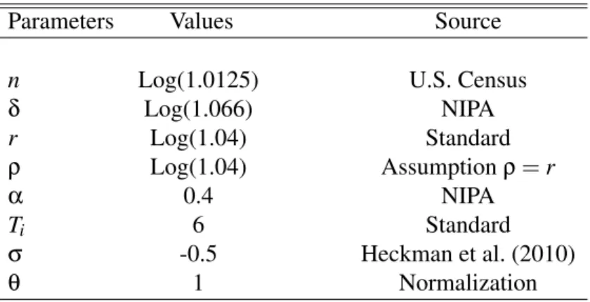
There is a group of parameters that are constant over time and are observed in the data. We follow the standard procedure of employing data from national accounts, the U.S. Census and values commonly used in the literature. The following table shows these parameters.
Parameters Values Source
n Log(1.0125) U.S. Census
δ Log(1.066) NIPA
r Log(1.04) Standard
ρ Log(1.04) Assumptionρ=r
α 0.4 NIPA
Ti 6 Standard
σ -0.5 Heckman et al. (2010)
θ 1 Normalization
Table 1: Observed parameters
The population growth rate,n, is the average U.S. population growth between 1900 and 2010, obtained from the U.S. Census. The National Income and Product Accounts (NIPA) provides the depreciation rate and the capital share in the goods sector, which are set to 6.6% and 40%, respec-tively13. The interest rate is set at 4%, and the parameterρhas the same value14. The first stage of the life cycle,Ti, is the pre-school period and is set at 6.
When studies on economic growth disregard early childhood education in the human capital accumulation, they implicitly assume that the two stages of human capital are substitutes. However, according to Heckman and Cunha (2007), an optimal allocation of human capital resources would be a distribution of investment between these stages. Thus, there is some degree of complementarity in the equation (5), i.e., parameterσshould be negative. Cunha et al. (2010) confirm the conclusion of Heckman and Cunha (2007). Indeed, with a nonlinear factor model with endogenous input, Cunha et al. (2010) estimate that the stages of human capital formation are complementary. Thus, the parameter that characterizes the complementarity of human capital function, σ, is set at -0.5, which is an intermediate value of Heckman et al. (2010) estimation15.
The model needs to set another group of variables to discipline and structure the shape of the U.S. economy. These parameters are life expectancy at birth, T, and retirement time, Tr, which
vary by year. Thus, the life expectancy at birth T for 1961, 1970, 1980, 1990, 2000 and 2008 was 70.27, 71.11, 74.01, 75.37, 76.74 and 77.94, respectively, which are the values reported in the World Development Indicators database. Additionally, the age of retirement for man was 61, 65, 63, 62, 63 and 63.45 for 1961, 1970, 1980, 1990, 2000 and 2008, respectively, which are the values
12Data restrictions explain the choice of 1961 as the first year. The last year is 2008 to avoid the financial crisis and
its consequences.
13For the depreciation rate, we use the long-run average for the investment/capital ratio.
reported in the Current Population Survey, 1962-2012 of the U.S. Bureau of the Census. Thus, the retirement time is the gap between life expectancy at birth and the age of retirement.
The remaining parameters to be calibrated are:
{A1,A2,A3,τK,τL,τH,τHc,γ,β,}
For each year, we have different distortions and TFP parameters but the same parameters of technology,γ, and preference,β. Thus, in total, we have 44 parameters to calibrate. To circumvent this hard task and to reduce the number of parameters, we normalizeA2to 1 and assume that some
parameters have a constant growth rate. Thus, we set
ξ(s) =ξ0eξg(s−2008), for
(
ξ∈ {A1,A3,τL,τH,τHc}
s∈ {1961,1970,1980,1990,2000,2008}
where the 0 superscript is the value for the year 2008, thegsuperscript is the growth rate, andsis the year16. With this simplification, we need to calibrate 13 parameters:
θ={A01,Ag1,A03,Ag3,τ0L,τLg,τ0H,τgH,τH0c,τgHc,τK,γ,β}
These parameters are calibrated so that in equilibrium, the model economy matches the follow-ing targets from the U.S. data:
i) GDP per capita in 2008 that is normalized to 1.
ii) Investment share of GDP in 2008 set to 0.2208 (Penn World Table).
iii) Share of early childhood sector workers in 2008 set to 0.0034 (OCDE statistics).
iv) Share of formal school sector workers in 2008 set to 0.0378 (OECD statistics).
v) Share of average worked hours in 2008 set to 0.3067 (OECD statistics).
vi) Average years of schooling in 2008 set to 13.2867 (Barro and Lee database).
vii) Mean of years of schooling for {1961,1970,1980,1990,2000,2008} set to 11.6987 (Barro and Lee database).
viii) Variance of years of schooling for{1961,1970,1980,1990,2000,2008}set to 2.4782 (Barro and Lee database).
ix) Mean of GDP per capita relative to 2008 for{1961,1970,1980,1990,2000,2008}set to 0.6763 (World Development Indicator)
x) Variance of GDP per capita relative to 2008 for {1961,1970,1980,1990,2000,2008} set to 0.0636 (World Development Indicator).
xi) Mean of average hours worked for{1961,1970,1980,1990,2000,2008}set to 0.3171 (OECD
statistics).
xii) Variance of average hours worked for {1961,1970,1980,1990,2000,2008}set to 9.185E-05 (OECD statistics).
xiii) Mean of GDP per capita growth rate between 1961 and 2008 set to 2.25% per year (World Development Indicators)
In this model, the output per capita of the economy is given by:
y=y1+q1y2+q2y3 (24)
Thus, we useyto match GDP per capita. The investment share of GDP is equal to(δ+n)kand the share of workers in each sector17 is given by equation (4).
As agents are homogeneous in our model, the average years of schooling is the optimum value ofTs that is implicitly set in the schooling decision, given by equation (11a) and (11b).
The life-cycle average labor supply of an individual is given by the labor supply throughout the life-cycle divided by the time that the individual could allocate to work. Therefore,
l= 1
T−Ty
Z Ty+Tw
Ty
l(ε)dε
This statistic matches the average hours worked. For this, we assume that there is a total of 16 hours of discretionary time per day18, which implies a total of 5840 (365*16) hours per year. Therefore, in 2008, we find that this statistic targeted a 1791/5840 ratio, where 1791 is the average hours worked in 2008.
Formally, the calibration strategy can be described as follows. Given a value forθ, we compute an equilibrium for each year s∈ {1961,1970,1980,1990,2000,2008} and define the following objects:
J1(bθ) =
V(ys(bθ)))−0.0636
E(ys(bθ))−0.6763
V(ls(bθ))−9.185E−05
E(ls(bθ))−0.3171
V(Tss(bθ))−2.4782
E(Tss(bθ))−11.6987
whereV(.)andE(.)indicate the variance and mean for years{1961,1970,1980,1990,2000,2008}. The second object that we define is
17It is represented byl
ifori∈ {1,2,3}.
J2(bθ) =
y2008(bθ) y1961(bθ)−e
0.0225(46)
y2008(bθ)−1
l2008(bθ)−0.3067
Ts2008(bθ)−13.2867
l22008(bθ)−0.0034
l32008(bθ)−0.0378
I2008(bθ)−0.2208
where the superscript indicates the year in which the respective variable was taken.
The first component of this vector indicates that between 1961 and 2008, the GDP per capita grew at a rate of 2.25% per year. The other terms are GDP per capita, life-cycle labor supply, years of schooling, share of workers in secondary and tertiary sectors and investment/GDP ratio, in this order.
Then, to findθ, we solve the following minimization problem:
min
θ J
⊤
1(θ)J1(θ) +J2⊤(θ)J2(θ)
Table 2 summarizes the results of our endogenous calibration. The model matches the targets very well. For instance, GDP per capita in 2008 is the worst match, but in this case, the error is only 2%. Furthermore, the objective function value of the minimization problem is 8.2E-04, and the average percentage error–the gap between the U.S. data and the model–is 0.48%. Thus, the model reproduces the U.S. data very well.
Parameter Value Target U.S. data Model
Leisure preference β 0.65 Mean of average hours worked to sample 0.317 0.316
Weight of early childhood
in Human Capital Technology γ 0.013 Mean of schooling to sample 11.7 11.67 Initial Labor Tax τ0
L 0.7 Average hours worked in 2008 0.307 0.308
Capital Tax τK 0.45 Investment share in 2008 0.22 0.22
Initial Schooling Tax τ0
H 0.6 Years of schooling in 2008 13.29 13.33
Initial Early Childhood Education Tax τ0
Hc 1.21 Worker share in sector 2 in 2008 0.0034 0.0034
TFP Initial Goods sector A01 0.42 GDP per capita in 2008 1 1.02 TFP Initial Schooling sector A0
3 2.3 Worker share in sector 3 in 2008 0.0378 0.0378 Trend of TFP goods sector Ag1 0.0078 Variance GDP per capita to sample 0.0636 0.0629 Trend of TFP schooling sector Ag3 -0.0089 Mean GDP per capita growth rate between 1961 to 2008 0.0225 0.0228 Trend of labor tax τgL -0.0001 Variance of average hours worked to sample 0.0001 0.0001
Ttrend of schooling tax τgH -0.024 Variance of schooling to sample 2.478 2.477
Trend of early childhood education tax τgHc -0.06 Mean GDP per capita to sample 0.676 0.678 Note: This sample is given by{1961,1970,1980,1990,2000,2008}.
Table 2: Endogenous parameters
4
Results
dynamics of the model is given by changing parameters{A1,A3,τL,τH,τHc}and the demographic
distribution, which is given by retirement age and life expectancy at birth.
(a) Years of schooling (b) GDP per capita
(c) Hours worked
Figure 1: Model and U.S. data - 1961 to 2008
The blue and red lines are, respectively, the model’s results and U.S. data. The model results are very close to the U.S. data. The average model error in absolute terms for school, GDP and hours worked are 0.76%, 1.92% and 1.43%, respectively 19. It is interesting to note that the fit for schooling and hours worked is surprisingly good because we use little information for the first years of these series20. For instance, in the 1960s the average error in absolute terms was 0.23% and 1.96%, for school and hours worked, respectively. Furthermore, for 1961, the first year of our series, the average error for these series were 0.68% and 1.87%, in this order21.
4.1
Relative Prices
In our model there is a rise in the relative prices of education that is supported by U.S. data. The main mechanism causing this rise is the relative increase in the labor productivity of the goods sector. The estimated reduction on the TFP of sector 3 and the increase in sector 1 over time help explain the increase22.
19The variance of these errors is 6.14-E05, 2.66-E04 and 7.92-E05, respectively. 20For example we do not use information to 1961 as a target.
21As robustness check for our calibration, we also calibrate and simulate the model for other two set of years: i)
Set1={1961,1962,1963,· · ·,2006,2007,2008}; and ii)Set2={1961,1965,1970,1980,· · ·,2000,2005,2008}. Table
5 in the appendix shows that the parameters are very close to the last calibration, and a simulation shows that the model is still good to fit the U.S. data. Indeed, the average error in absolute terms for schooling, GDP and hours worked is, respectively, 0.78%, 1.99% and 1.42% forSet1and 0.89%, 1.83% and 1.42% forSet2.
22This is supported by results in Hanushek and Rivkin (1997). Indeed, Hanushek and Rivkin (1997, p.37) stat “The
(a) Model prices (b) Prices index for U.S. economy - Bureau of Labour Statistics
Figure 2: Model and Data prices - 1978 to 2008
Figure 2 shows the relative prices of the model and the price index for the U.S. economy. To relate the prices of our model (figure 2a) with the data prices (figure 2b) note that the variables "all items", "durables goods" and "housing" are associated with the goods sector, while the variables "services", "educational books and supplies", "tuition other school fees and childcare", "college tuition and fees and elementary" and "high school tuition and fees" are associated with the edu-cation sector. It is clear from figure 2b that the prices associated with eduedu-cation sector increased faster than the prices associated with the goods sector, which supports the results of our model. Indeed, in the U.S. data, the index price of "all items", "durables goods" and "housing" increased 3.3, 1.62 and 3.46 times, respectively, while the index price of "services", "educational books and supplies", "tuition, other school fees and childcare", "college tuition and fees and elementary" and "high school tuition and fees" increased 4.2, 7.3, 8.73, 9.55 and 9.62 times, respectively. In our model, the relative prices of formal and early childhood education increased 93.07% and 47.9%, respectively.
We conduct an experiment of the model with TFP parameters to measure the importance of the relative prices in our quantitative results. Basically, we keep only the values of the TFP parameters (A1andA3) constant at their 2008 levels, changing the others.
When we keep constant the TFP parameters at their 2008 levels, the prices of education for the other years are higher than in the calibrated model. This increased price would have an expressive impact on educational choices. For all years, formal education and early childhood education would be lower in the experiment. In 1961, where we have the biggest gap between the experiment and the calibrated model, the results of experiment for formal and early childhood education would be 60.48% and 55.18% below the results of calibrated model, respectively23.
In Restuccia and Vandenbroucke (2013a), the growth of wages, which is given exogenously, is the main factor explaining the evolution of years of schooling in the U.S. economy. In our model, however, the growth of wages is given endogenously, and TFP parameters are the exogenous force that could affect the wages. What is important in our model for schooling choices is the growth of wages relative to tuition costs24,w/qifori∈ {1,2}. In this way, the impact of the TFP of the goods
sector in schooling is insignificant because it affects only the level of wages and does not affect the
to be a prime example, that experiences little technological change while other sectors undergo regular productivity improvements. Because wages rise roughly in proportion with the average growth rate of labor productivity in all sectors, the technologically stagnant sector faces increased labor costs.”
23In 1961 the TFP experiment increased the prices of early childhood education and formal education by 1.85 and
2.8 times, in this order.
ratio of wages to tuition costs25.
5
The Driving Forces
To better understand our results, we quantitatively decompose the contribution of exogenous vari-ables to the variation in human capital and income. We measure the effect of distortionsτL,τH and
τHc and life expectancy,T, on GDP per capita, schooling and early childhood education. For this,
we keep the value of one parameter constant at the 2008 level, changing the others.
(a) Years of schooling (b) Early Childhood Education
(c) GDP per capita
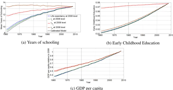
Figure 3: Constant level at 2008 for some exogenous variables - 1961 to 2008
Figure 3 presents the results. The main point is the large effect of educational distortions and the smaller effect of labor distortions and life expectancy. The explanation is straightforward. While the life expectancy increased 10.91% and the labor distortions reduced 0.57% from 1961 to 2008, the measured schooling and early childhood education distortions reduced by 68.09% and 92.77%, respectively.
We can note from figure 3a that the schooling distortion was the most important force of rising years of schooling. Indeed, when we keep constant the schooling distortion at its 2008 level,τ2008
H ,
the formal education is approximately constant at the 2008 level.
The experiment with early childhood distortion,τHc, shows the importance of early childhood
education to schooling. Indeed, due to an exogenous reduction inτHc, early childhood education in
1961 would be close to its measured level in 200826, which would increase the return of one extra year in formal school; therefore, schooling would also increase. Quantitatively, the impact would be large: In 1961, schooling would be just 11.29% below the 2008 level, while in the baseline simulation it would be 31.2% below.
25It is necessary to clarify that in this case, the result in GDP per capita is too large. For example, in 1961, the GDP
per capita increased 84.61% with respect to the calibrated model.
26In the early childhood experiment in figure 3b, the 1961 early childhood level would have been 87% the 2008
Although life expectancy affects schooling, its contribution is not too large. For instance, if in 1961 the life expectancy had been 77.94 years – the 2008 level – schooling would have been 9.62. Thus, when life expectancy increased 10.92%, years of schooling increased only 4.91%. This result shows that life expectancy was not an important force to explain the schooling evolution. This result agrees with part of the literature. For example, in Restuccia and Vandenbroucke (2013a) and Restuccia and Vandenbroucke (2013b), life expectancy is the least important exogenous force to explain schooling evolution.
In Ferreira and Pessoa (2007) life expectancy has a larger effect on schooling than it does here. This is because the human capital choice is based only on formal schooling decision, while we also have one intensive margin, early childhood education. Hence, the interaction between early childhood education and years of schooling reduces the effect of life expectancy on schooling. Figure 3b shows that in 1961, early childhood would have increased by 6.97% if life expectancy had increased 10.92%.
Figure 3 also shows that the impact of labor distortion was small. From 1961 to 2008, formal education increased 45.34% in our calibrated results. However, if the value of labor distortion parameter had been fixed at the 2008 level, formal education would have increased 41.26%. The results for early childhood education are similar. Thus, distortions to labor were not important to explain U.S. education.
Figure 3c presents the GDP per capita in our simulations. The interesting fact is that childhood education is as important as formal education to explain the evolution of GDP per capita. Indeed, in 1961, theτHcexperiment increased (when compared to the baseline) scenario, the income per capita
by 43.67%, while theτH experiment increased the income per capita by 37.72%. The main factor
behind this result is the impact on labor productivity. Early childhood is very important for labor productivity due the interaction with formal education, so the large evolution of early childhood27 was essential to understand the increase in labor productivity in the U.S. economy28. Furthermore, the expansion of human capital increased the opportunity cost of leisure29, leading to an increase in labor effort, which in turn amplified even further the impact of human capital on output.
Life expectancy and the labor distortion had a small role in explaining the evolution of income. Changing life expectancy (blue line) and labor distortions (green line) in 1961 to their 2008 levels increased income only 2.2% and 3.71%, in this order.
6
Economic Development and Distortions
Distortions to the accumulation of human capital play a key role in our model. These wedges are reduced-form parameters that encompass barriers to educational investments that are not directly reflected in prices. They can represent, e.g., policy distortions, barriers to the adoption of best practices or technology, bad management, and high commuting costs. In our model, they affect different activities and sectors in different ways; there is heterogeneity across educational stages. It would thus be interesting to investigate the relative impact of these distortions on human capital accumulation, on output and each one of them is more harmful to labor productivity.
27Between 1961 and 2008, early childhood increased 6.46 times.
28It is important to remember that the weight of early childhood education in human capital function,γ, was 0.013,
and so, the schooling weight was 0.987. Although it implies a priori a small value of return of early childhood investment, the dynamic effect of complementarity in human capital formation leads early childhood education be used as input for formal education, which improves the return in formal education.
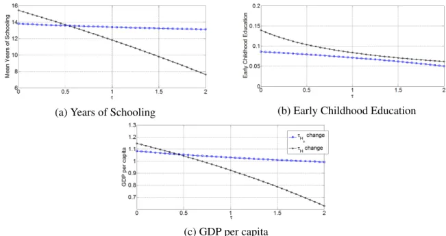
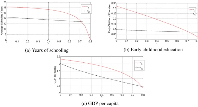
Figure 4c compares the impact of different types of educational distortion on both education and GDP per capita, holding all other parameters constant at their 2008 level. It is straightforward from figure 4c that GDP per capita is more sensible to formal education distortion than to early childhood distortion. The arc elasticity of formal education distortion (black line) and of early childhood distortion (blue line) is -0.52 and -0.092, respectively.
(a) Years of Schooling (b) Early Childhood Education
(c) GDP per capita
Figure 4: Impact of different types of educational distortion on both education and GDP per capita
Figure 4a and 4b may help us understand these results. Distortion to formal education causes a larger variation in years of schooling than does distortion in early childhood education (figure 4a), while the impact of both distortions on early childhood education are close (figure 4b). Indeed, whenτHincreases from 0 to 2, schooling years and early childhood education decrease by 51% and
41.62%, respectively, while in the τHc experiment, schooling years and early childhood education
decrease by 5% and 56%, respectively.
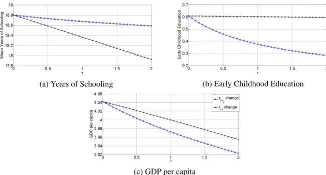
In figure 5, we have a similar analysis but in an economy without distortions (τi=0 for i∈
{L,K,H,Hc}). We have a different picture here: GDP per capita is less sensible to formal education
distortion than to early childhood distortion. Now, the arc elasticity of formal education distortion (black line) and that of early childhood distortion (blue line) are -0.088 and -0.12, respectively. This mainly happens because labor distortions amplify the effects of formal education distortion. In fact, labor distortions act in the same way that formal education distortions do because both distortions affect the time allocation in the educational stage (extensive dimension).
(a) Years of Schooling (b) Early Childhood Education
(c) GDP per capita
Figure 5: Impact of different types of educational distortion on both education and GDP per capita in a model initially without distortions
be more attractive than early childhood education, which amplifies the effects of formal education distortion vis-à-vis early childhood distortion. The opposite occurs in an economy without distor-tion: The high opportunity cost makes the early childhood investment (intensive dimension) more attractive, and thus, the impact of early childhood distortion becomes stronger.
The results in figures 4 and 5 highlight the fact that general equilibrium effects on human capital investment should be taken into account in the evaluation of the relative impact of policies targeted toward different educational stages. Some papers document that in a bad environment for children, it is better to invest more in the early stages of childhood than later (Heckman et al., 2013; Heckman and Cunha, 2007; Cunha et al., 2010). We conduct an experiment that intend to mimic a scenario in which there is a configuration of disadvantages for children. We thus analyze the impact of distortions if the level of early childhood distortion in 2008 were the same of 1961 (τHc=τ
1961
Hc ),
i.e., we analyze our economy in a bad scenario for early childhood. In this case, if the distortion in early childhood decreased 10%, the income would increase 2%, but if the distortion in the formal education decreased 10%, the income would increase only 1.95%. To clarify the importance of economic structure for opportunity cost, we set τL =0 in the last analysis. Thus, if distortion in
the early and later education decreased 10%, income would increase 0.67% and 0.1%, respectively. Thus, we confirm the results in the literature and show that it is strengthened whenτL =0.
Figure 6 shows the impact of changes on labor and capital distortion for years of schooling, early childhood education and GDP per capita.
(a) Years of schooling (b) Early childhood education
(c) GDP per capita
Figure 6: Impact of different types of labor and capital distortion on education and GDP per capita
7
Sensitivity
In this section, we conduct two sensitivity analyses. First, we analyze the sensitivity of the results with respect to complementarity parameterσ. After that, we change our model to incorporate more directly the role of government in education.
7.1
Complementarity
In this section, we analyze the sensitivity of the results with respect to complementarity parameter
σ. Studies on human capital formation claim that investments across stages of cognitive devel-opment are complementary, i.e., early investment increases the productivity of later investment (Cunha et al., 2006; Heckman and Cunha, 2007; Heckman et al., 2010). We simulate the model with the following parameter of complementarity : σ∈ {−1,−0.75,−0.25,−0.01,0.01}, remak-ing the calibration procedure for each differentσ. The parameters are shown in table 3.
Complementarity β γ τ0
L τK τ0H τ
0
Hc A
0
1 A03 A
g
1 A
g
3 τ
g
L τ
g H τ
g Hc σ=-1 0.64 0.003 0.71 0.45 0.57 1.15 0.41 2.20 0.0087 -0.011 -0.00009 -0.029 -0.042
σ=-0.75 0.65 0.006 0.70 0.45 0.61 1.25 0.42 2.25 0.0086 -0.011 -0.00009 -0.030 -0.040
σ=-0.5 0.65 0.013 0.70 0.45 0.60 1.21 0.42 2.30 0.0078 -0.009 -0.00012 -0.024 -0.056
σ=-0.25 0.65 0.028 0.70 0.45 0.61 1.14 0.43 2.39 0.0068 -0.008 -0.00016 -0.020 -0.075
σ=-0.01 0.67 0.06 0.69 0.45 0.67 1.21 0.45 2.55 0.0061 -0.012 -0.00012 -0.028 -0.100
σ=0.01 0.66 0.062 0.70 0.45 0.66 1.10 0.45 2.55 0.0063 -0.012 -0.00011 -0.029 -0.100
There is a negative correlation betweenγ– the weight of early childhood education in human capital function – and σ. Moreover, γ fluctuates considerably withσ. This makes sense because investment in formal education is more attractive when it increases the elasticity of the substitution of human capital – when the value of σ increases – because the individual needs to discount the future less than early childhood investment. However, remember that we have the same target for schooling. Thus, the weight of schooling, 1−γ, needs to decrease as it compensates for the increase in the return of schooling, i.e., the weight of early childhood education needs to increase.
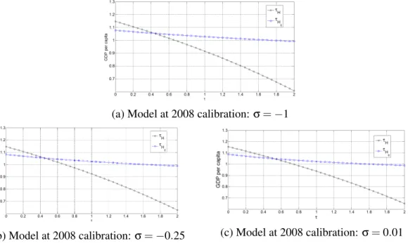
Figure 7 presents the sensitivity of the results of Section 6 for eachσ∈ {−1,−0.25,0.01}. We conclude that the results of the calibrated model are robust toσ30. Indeed, the distortion of formal education affects the income per capita more than the distortion of early childhood education.
(a) Model at 2008 calibration:σ=−1
(b) Model at 2008 calibration: σ=−0.25 (c) Model at 2008 calibration:σ=0.01
Figure 7: Impact of different types of education distortion on GDP per capita - sensitivity analysis
7.2
Introducing Public Expenditures on Education
One possible interpretation of the distortions to/incentives for human capital accumulation is that they are a measure of, among other things, the impact of government policies. It would be in-teresting, however, to incorporate a direct role of the government in affecting education. This is performed, in this section, by adding public investment to the human capital functions (equation (5)).
We consider that investment in education now has private and public sources. The human capital function of early education is now given by:
h1(x,g1) =(xTi)η+ (g1Ti)η 1
η
(25)
where g1 is government investment in early education, and η is the parameter that characterizes
the elasticity of substitution between private and public goods31. The human capital in the second stage is now given by:
h(Ts,x) =
γh1(x,g1)σ+ (1−γ)h2(Ts,g2)σ
1
σ
(26)
whereh2is:
h2(Ts,g2) =
Tsη+ (g2Ts)η 1
η
(27) In the function above, g2 is government investment in formal education. Note that as in the
previous case, the human capital accumulated in the first stage is a component of the human cap-ital function of the second stage. Equation (15), the distortions/budget constraint equation of the government, is modified to:
τLwl(s,s)h(Ts,x)Nw+τKRκ+ (τHcx−g1)q1Ni+ (τH−g2)q2Ns=χ (28)
There are no data on government expenditure on pre-primary education before the nineties, so we estimate this series. First, we calculate the mean share of government expenditure on pre-primary to pre-pre-primary through secondary education between 1998 and 2008, which is available in the UNESCO database. We then use pre-primary through secondary education expenditures as percentage of GDP, available in theUS Government Spending database, for the years prior to 1998, and keep constant the estimated share of government expenditure on pre-primary education to estimate the government expenditure of pre-primary education between 1971 and 1997. Finally, we use student enrollment in both pre-primary and primary + secondary education, also available in theUNESCOdatabase, to calculate the ratio of government expenditure per student to GDP per capita in each educational stage32.
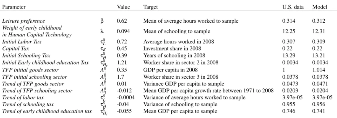
We calibrate this model to fit the U.S. economy following the previous procedure discussed in the calibration section33. Table 6 summarizes the result. As before, the model matches the targets very well. GDP per capita in 2008 is the worst match, but in this case, the error is only 1.4%.
Note that the calibration is not too sensitive to these changes. Indeed, only the distortion to formal education and the weight of early childhood education in the human capital function (γ) changed significantly. This happened because the government expenditure per student on late ed-ucation increased over time relative to early childhood eded-ucation. Therefore, distortions in late childhood education capture this fact and, thus, are lower than in the benchmark model.
The largest share of total government expenditure on pre-primary education was observed in 2000, which was 9.7% of government expenditure between pre-primary and secondary education. Therefore, if we kept constant total government expending on education but increased by 10%, for all years, the share of total government expenditure on pre-primary education34, the income per capita would be higher for all years, but it would be only 0.1% higher on average.
31This formulation of human capital is similar to Blankenau and Youderian (2015); thus, we setη=0.48, which is
the calibrated value from this article.
32Figure 8 in the appendix presents the government expenditures on education. 33Due to data restrictions, we use only the sample{1971,1980,1990,2000,2008}.
34In this case, the government would spend, on average, 10.36% more with pre-primary students and 0.99% less
Parameter Value Target U.S. data Model
Leisure preference β 0.62 Mean of average hours worked to sample 0.314 0.312
Weight of early childhood
in Human Capital Technology λ 0.094 Mean of schooling to sample 12.25 12.31 Initial Labor Tax τ0
L 0.72 Average hours worked in 2008 0.307 0.309
Capital Tax τK 0.45 Investment share in 2008 0.22 0.22
Initial Schooling Tax τ0
H 0.39 Years of schooling in 2008 13.29 13.21
Initial Early childhood education Tax τ0
Hc 1.21 Worker share in sector 2 in 2008 0.0034 0.0034
TFP initial goods sector A0
1 0.35 GDP per capita in 2008 1 1.014 TFP initial schooling sector A03 1.7 Worker share in sector 3 in 2008 0.0378 0.0378 Trend of TFP goods sector Ag1 0.01 Variance GDP per capita to sample 0.0473 0.0471 Trend of TFP schooling sector Ag3 -0.012 Mean GDP per capita growth rate between 1971 to 2008 0.0203 0.0204
Trend of labor tax τgL -0.0004 Variance of average hours worked to sample 3.97e-05 3.97e-05
Trend of schooling tax τgH -0.04 Variance of schooling to sample 0.955 0.956
Trend of early childhood education tax τgHc -0.055 Mean GDP per capita to sample 0.746 0.741
Note: This sample is given by{1971,1980,1990,2000,2008}.
Table 4: Endogenous parameters - Government expenditure per student as percentage of GDP per capita
We also reanalyze Section 6, and the results do not change: Income per capita is more sensitive to formal education distortions than to early childhood distortions. This result is not contradictory to the previous result because in this case, government investment increases the amount of goods that are used directly in human capital function, while educational distortions affect the prices of education that is privately purchased.
Following Blankenau and Youderian (2015), we change (and recalibrate) our model to use, as they do, government expenditure on education as a percentage of GDP instead of expenditure per student. Therefore, if in 2008 the government expenditure on pre-primary education had been 0.004 higher (+0.4% of GDP), income per capita would have been 8.62% higher, which is near what they found in their article. Moreover, if the government reallocated expending such that it were equal among pre-primary, primary and secondary education, income per capita would be 2.19% higher. This very strong result is due to their use of total public expenditure and disappears once one uses public expenditure per student.
8
Conclusion
In this paper, we have studied the evolution of human capital of American workers between 1961 and 2008. The new approach is that we have brought early childhood studies to our work, and thus, we have been able measure the evolution of early childhood human capital and its importance in labor productivity. In addition, we can understand and measure how distortions in education, labor and capital choice have affected U.S. development. We conclude that early childhood human capital increased 6.46 times between 1961 and 2008, and the share of early childhood human capital in the labor productivity increased 3.88 times. Furthermore, reduction in the early childhood distortion was the main force to understand income per capita evolution, leaving behind other exogenous forces, such as reduction in the formal education distortion and increased life expectancy.
of formal education is formed by opportunity cost and tuition cost, while the marginal cost of early childhood education is only tuition cost. Thus, in a scenario where distortions are zero, these result will change because the opportunity cost will be much higher.
We also have changed our model to analyze government incentives in education. The main result is the U.S. government would have increased income per capita only with a reallocation of educational resources for early childhood education.
References
Abington, C. and W. Blankenau (2013). Government education expenditures in early and late childhood. Journal of Economic Dynamics and Control 37(4), 854–874.
Attanasio, O. P. (2015). The determinants of human capital formation during the early years of life: Theory, measurement, and policies. Journal of the European Economic Association 13(6), 949–997.
Baumol, W. J. (1967). Macroeconomics of unbalanced growth: the anatomy of urban crisis. The American economic review, 415–426.
Baumol, W. J. and W. G. Bowen (1965). On the performing arts: the anatomy of their economic problems. The American Economic Review 55(1/2), 495–502.
Ben-Porath, Y. (1967). The production of human capital and the life cycle of earnings.The Journal of Political Economy, 352–365.
Blankenau, W. and X. Youderian (2015). Early childhood education expenditures and the intergen-erational persistence of income. Review of Economic Dynamics 18(2), 334–349.
Carneiro, P. M. and J. J. Heckman (2003). Human capital policy.
Castro, R. and D. Coen-Pirani (2014). Explaining the evolution of educational attainment in the us.
Córdoba, J. C. and M. Ripoll (2013). What explains schooling differences across countries? Jour-nal of Monetary Economics 60(2), 184–202.
Cunha, F., J. J. Heckman, L. Lochner, and D. V. Masterov (2006). Interpreting the evidence on life cycle skill formation. Handbook of the Economics of Education 1, 697–812.
Cunha, F., J. J. Heckman, and S. M. Schennach (2010, 05). Estimating the Technology of Cognitive and Noncognitive Skill Formation. Econometrica 78(3), 883–931.
Del Boca, D., C. Flinn, and M. Wiswall (2014). Household choices and child development. The Review of Economic Studies 81(1), 137–185.
Erosa, A., T. Koreshkova, and D. Restuccia (2010). How important is human capital? a quantitative theory assessment of world income inequality. Review of Economic Studies 77(4), 1421–1449.
Hanushek, E. A. and S. G. Rivkin (1997). Understanding the twentieth-century growth in us school spending. INTERNATIONAL LIBRARY OF CRITICAL WRITINGS IN ECONOMICS 159(2), 204–240.
Heckman, J. and F. Cunha (2007, May). The Technology of Skill Formation. American Economic Review 97(2), 31–47.
Heckman, J., R. Pinto, and P. Savelyev (2013, October). Understanding the Mechanisms through Which an Influential Early Childhood Program Boosted Adult Outcomes. American Economic Review 103(6), 2052–86.
Heckman, J. J. (2011). The economics of inequality: The value of early childhood education.
American Educator 35(1), 31–35.
Heckman, J. J., S. H. Moon, R. Pinto, P. Savelyev, and A. Yavitz (2010, July). A New Cost-Benefit and Rate of Return Analysis for the Perry Preschool Program: A Summary. NBER Working Papers 16180, National Bureau of Economic Research, Inc.
Irwin, L. G., A. Siddiqi, and C. Hertzman (2007). Early child development: a powerful equalizer.
Vancouver, BC: Human Early Learning Partnership and World Health Organization.
Klenow, P. J. and M. Bils (2000, December). Does Schooling Cause Growth? American Economic Review 90(5), 1160–1183.
Knudsen, E. I., J. J. Heckman, J. L. Cameron, and J. P. Shonkoff (2006). Economic, neurobio-logical, and behavioral perspectives on building america’s future workforce. Proceedings of the National Academy of Sciences 103(27), 10155–10162.
Lee, D. and K. I. Wolpin (2010). Accounting for wage and employment changes in the us from 1968–2000: A dynamic model of labor market equilibrium. Journal of Econometrics 156(1), 68–85.
Manuelli, R. E. and A. Seshadri (2014). Human capital and the wealth of nations. The American Economic Review 104(9), 2736–2762.
Myers, R. and X. de San Jorge (1999). Childcare and early education services in low-income communities in mexico city: Patterns of use, availability and choice.
Rangazas, P. (2000). Schooling and economic growth: a king–rebelo experiment with human capital. Journal of Monetary Economics 46(2), 397–416.
Rangazas, P. (2002). The quantity and quality of schooling and us labor productivity growth (1870– 2000). Review of Economic Dynamics 5(4), 932–964.
Restuccia, D. and R. Rogerson (2008). Policy distortions and aggregate productivity with hetero-geneous establishments. Review of Economic Dynamics 11(4), 707–720.
Restuccia, D. and C. Urrutia (2004). Intergenerational persistence of earnings: The role of early and college education. American Economic Review, 1354–1378.
Restuccia, D. and G. Vandenbroucke (2013b). The Evolution Of Education: A Macroeconomic Analysis. International Economic Review 54, 915–936.
Restuccia, D. and G. Vandenbroucke (2014). Explaining educational attainment across countries and over time. Review of Economic Dynamics 17(4), 824–841.
Rolnick, A. and R. Grunewald (2003). Early childhood development: Economic development with a high public return. The Region 17(4), 6–12.
Schoellman, T. (2012). Education quality and development accounting. The Review of Economic Studies 79(1), 388–417.
Schoellman, T. (2014). Early childhood human capital and development.
Schweinhart, L. J. (2004). The High/Scope Perry Preschool study through age 40: Summary, conclusions, and frequently asked questions. High/Scope Educational Research Foundation.
Scitovsky, T. and A. Scitovsky (1959). What price economic progress? Yale Law Review 49, 95–110.
You, H. M. (2014). The contribution of rising school quality to u.s. economic growth. Journal of Monetary Economics 63(0), 95 – 106.