www.geosci-model-dev.net/9/1545/2016/ doi:10.5194/gmd-9-1545-2016
© Author(s) 2016. CC Attribution 3.0 License.
The ecological module of BOATS-1.0: a bioenergetically constrained
model of marine upper trophic levels suitable for studies of fisheries
and ocean biogeochemistry
David Anthony Carozza1, Daniele Bianchi1,2,a, and Eric Douglas Galbraith1,b,c
1Department of Earth and Planetary Sciences, McGill University, Montreal, Canada 2School of Oceanography, University of Washington, Seattle, Washington, USA
anow at: Department of Atmospheric and Oceanic Sciences, University of California, Los Angeles, California, USA bnow at: Institució Catalana de Recerca i Estudis Avançats (ICREA), 08010 Barcelona, Spain
cnow at: Institut de Ciència i Tecnologia Ambientals (ICTA) and Department of Mathematics,
Universitat Autonoma de Barcelona, 08193 Barcelona, Spain
Correspondence to:David Anthony Carozza (david.carozza@gmail.com)
Received: 11 October 2015 – Published in Geosci. Model Dev. Discuss.: 1 December 2015 Revised: 14 March 2016 – Accepted: 1 April 2016 – Published: 22 April 2016
Abstract.Environmental change and the exploitation of ma-rine resources have had profound impacts on mama-rine commu-nities, with potential implications for ocean biogeochemistry and food security. In order to study such global-scale prob-lems, it is helpful to have computationally efficient numeri-cal models that predict the first-order features of fish biomass production as a function of the environment, based on empir-ical and mechanistic understandings of marine ecosystems. Here we describe the ecological module of the BiOeconomic mArine Trophic Size-spectrum (BOATS) model, which takes an Earth-system approach to modelling fish biomass at the global scale. The ecological model is designed to be used on an Earth-system model grid, and determines size spec-tra of fish biomass by explicitly resolving life history as a function of local temperature and net primary production. Biomass production is limited by the availability of photo-synthetic energy to upper trophic levels, following empirical trophic efficiency scalings, and by well-established empiri-cal temperature-dependent growth rates. Natural mortality is calculated using an empirical size-based relationship, while reproduction and recruitment depend on both the food avail-ability to larvae from net primary production and the pro-duction of eggs by mature adult fish. We describe predicted biomass spectra and compare them to observations, and con-duct a sensitivity study to determine how they change as a function of net primary production and temperature. The
model relies on a limited number of parameters compared to similar modelling efforts, while retaining reasonably realistic representations of biological and ecological processes, and is computationally efficient, allowing extensive parameter-space analyses even when implemented globally. As such, it enables the exploration of the linkages between ocean bio-geochemistry, climate, and upper trophic levels at the global scale, as well as a representation of fish biomass for idealized studies of fisheries.
1 Introduction
re-ductions (local extinctions) (McCauley et al., 2015), and an index of marine finfish biomass indicates an aggregate loss of 38 % over many species (Hutchings et al., 2010). Despite increasing harvesting effort (Watson et al., 2013b), annual wild harvest appears to have peaked globally in the early 1990s (Watson et al., 2004; Pauly, 2007; FAO, 2014) at an annual rate that has been recently estimated at 130 million tonnes (Mt) per year (Pauly and Zeller, 2016), since which time it appears to have declined. As older coastal fisheries have become increasingly depleted (Jackson, 2001), harvest has extended to more taxa as well as further from the coast and deeper in the water column (Norse et al., 2012; Watson and Morato, 2013).
Anthropogenic climate change, on the other hand, is al-ready altering nutrient dynamics and primary production through its effects on ocean temperature and circulation (Doney et al., 2012), with demonstrated consequences on the distributions of several fish populations (Pinsky et al., 2013; Walsh et al., 2015). Global climate models suggest that increased surface water stratification due to warming could decrease nutrient upwelling and so reduce net pri-mary production (Sarmiento et al., 2004; Steinacher et al., 2010; Bopp et al., 2013). Warming can also directly influence fish biomass by affecting physiological rates that influence growth, mortality, reproduction, recruitment, and migration (Brander, 2010; Sumaila et al., 2011). Despite progress in identifying important mechanisms of biomass change, portant uncertainties remain in constraining the overall im-pact and the spatial distribution of change in net primary production (Taucher and Oschlies, 2011) and fish biomass, with current analyses pointing toward heterogeneous spa-tial change in fish production and harvest potenspa-tial (Cheung et al., 2010; Barange et al., 2014; Lefort et al., 2014).
Research in fisheries and fisheries economics often fo-cusses on particular species, regions, and markets. In recent years, generalized, spatially resolved models of the marine ecosystem applicable to the global domain have been de-veloped, but most are not directly coupled with predictive models of fishing activity (Jennings et al., 2008; Lefort et al., 2014; Watson et al., 2014). Our intention is to model fisheries and economic harvesting as parts of an integrated system that is bioenergetically constrained, and based on fundamen-tal physical, ecological, and economic principles. The eco-logical module of the BiOeconomic mArine Trophic Size-spectrum model (BOATS) aims to represent commercial or-ganisms as a set of super-organism populations (that we refer to as groups) that grow, reproduce, and die, taking into ac-count their dependence on local environmental variables in the framework of a two-dimensional grid of the global ocean. The approach is structurally simpler than that of Christensen et al. (2015), and bears similarity with that of Jennings and Collingridge (2015), but unlike these models the BOATS ecological model explicitly treats life history and reproduc-tion, similar to Maury et al. (2007).
The true ecological structure of marine communities is very complex, and includes many species-level ecological dynamics that are not understood at a mechanistic predic-tive level. A typical oceanic food web consists of dozens or more of interacting species, whose sizes span several or-ders of magnitude and whose lifetimes range from days to decades. Instead of attempting to model such species-level characteristics, we rely on the simple principle that the over-all growth of organisms within a community depends on the availability of energy from net primary production, relative to the total consumption of energy by the metabolic activ-ity of the communactiv-ity. Since one of our primary goals is to predict fishery harvest through coupling with an economic model, we define our community as including all commer-cially harvested organisms, including pelagic, demersal, and benthic species, both finfish and invertebrates (see discussion of size-based groups in the next section), referring to all as “fish” for simplicity.
In this paper, we describe the ecological module of the BOATS model. In a companion paper (Carozza et al., 2016), the ecological module is coupled to an economic harvesting module and extended to a two-dimensional global grid, in or-der to explore the spatial distribution of harvest as well as the parameter uncertainty. Here, we present in detail the equilib-rium biomass at two ocean sites using a single set of param-eter values, and conduct a sensitivity study to illustrate how the model biomass and the size structure of marine commu-nities depend on net primary production and temperature.
2 Fish ecology model
The ecological module of BOATS uses the McKendrick– von Foerster (MVF) model (McKendrick, 1926; von Foer-ster, 1959), a widely used continuous-time model for an age-or size-structured population, to represent the evolution of biomass. Populations of fish biomass (all of the organisms in a group) are organized by size and are described by a con-tinuous biomass distribution that we refer to as a biomass spectrum. Fish begin in the smallest size class and grow over time into adjacent (larger) size classes. In each size class, fish biomass evolves in time as the biomass growth less the natu-ral mortality.
rep-resents biomass losses due to predation, by organisms both within and outside of the community, as well as other natural causes. The mortality formulation depends on an empirical relationship that considers the individual mass of the fish, the asymptotic mass of the fish (the maximum theoretical mass), and the temperature. The addition of new biomass into the smallest mass class, referred to as recruitment, is determined as a function of the net primary production and the produc-tion and survival of eggs.
BOATS is designed with the global ocean in mind, yet for ease of reading we present it for a single patch of the ocean, or in other words, for a single grid point on a two-dimensional grid. By then applying BOATS to each oceanic grid cell independently, we represent fish biomass and har-vest on a two-dimensional global grid. We force biomass using two-dimensional grids of vertically integrated net pri-mary production (NPP) and vertically averaged temperature derived from satellite ocean colour and direct temperature measurements, respectively (Sect. 2.8). At each grid point, we therefore simulate biomass spectra that are independent of the adjacent grid points. Hence, we do not take active or passive movement of fish, larvae, or eggs between adjacent grid points into account. These are complex processes that have been shown to play a role in determining fish biomass distributions (Watson et al., 2014). In BOATS, we assume that fish are present where there is NPP to provide food. Given that the model grid cells are 1◦×1◦, we only ef-fectively ignore nonlocal movements that occur over spatial scales that are larger than approximately 100 km×100 km. This could bias our results in parts of the ocean where the advection of fish biomass is strong relative to the time step and spatial grid scale, such as in the Gulf Stream. This is es-pecially true for larvae, but would likely pose less of a prob-lem for larger fish since they swim faster than strong oceanic currents. Due to the movement of plankton by currents, a bias could also result from the difference in the locations at which plankton and fish production occur. We expect this to have a small impact on our results given our relatively coarse spa-tial resolution. Movement induced by ocean circulation and fish behaviour could be implemented in the future, with exist-ing advection and diffusion algorithms (Faugeras and Maury, 2005; Watson et al., 2014).
In the current implementation of the model, we consider three independent populations of fish at every grid point, and so resolve three biomass spectra. These populations, which we refer to as groups, are defined by their asymptotic sizes as small, medium, and large fish, which allows for a very crude representation of biodiversity (Andersen and Beyer, 2006; Maury and Poggiale, 2013). There is no growth from one group to another; in other words, the small group consists of fish that remain small throughout their life history, such as anchovies and sardines, and so are distinct from the juve-niles of the medium and large groups. The asymptotic mass, the mass at which all energy is allocated to reproduction and therefore the mass at which growth stops, characterizes each
group. We employ groups since they allow us to make use of well-studied growth and mortality characteristics of fish of different asymptotic size (Andersen and Beyer, 2006; Maury and Poggiale, 2013). We work with a finite number of groups as opposed to a continuum (as in Andersen and Beyer, 2006; Maury and Poggiale, 2013), to directly compare our har-vest results to the Sea Around Us Project (SAUP) harhar-vest database (Watson et al., 2004; Pauly, 2007), using the three asymptotic masses (Sect. 2.9) from the functional group defi-nitions of the SAUP harvest database. Our group formulation combines functional groups (pelagic, demersal, and benthic, for example). Such an assumption may not be appropriate for particular aspects of benthic ecosystems, which have been shown to require more than a representation of size structure to adequately represent core ecosystem features (Duplisea et al., 2002; Blanchard et al., 2009). Nevertheless, for our global-scale model, we feel justified in using such a group formulation since Friedland et al. (2012) found little differ-ence in how the biogeochemical attributes and harvest of pelagic and demersal fisheries reacted to primary production and trophic transfer efficiencies. Alternative group formula-tions remain a promising avenue of research in global fish-eries modelling, one that could be pursued in future work (Blanchard et al., 2009; Maury, 2010).
Although we use the classical MVF model, we implement empirical relationships whenever possible to determine fun-damental rates such as growth and mortality, since our goal is to represent fish biomass at the global scale, while limiting the model complexity and number of parameters. As opposed to determining both growth and mortality from explicit pre-dation, as in Maury et al. (2007), Blanchard et al. (2009), Hartvig et al. (2011), and Maury and Poggiale (2013), NPP and the size distribution of phytoplankton set growth rates for all mass classes of fish through a trophic transfer of en-ergy from phytoplankton to fish. To guarantee that growth rates do not exceed realistic values, a von Bertalanffy growth formulation that is based on field observations acts as an up-per limit to the growth rate (von Bertalanffy, 1949; Hartvig et al., 2011; Andersen and Beyer, 2013). Mortality is based on an empirical parameterization that depends on mass and asymptotic mass, but also on the constant allometric growth rate in the empirical limit (Gislason et al., 2010; Charnov et al., 2012).
MVF model. APECOSM (the Apex Predators ECOSystem Model, Maury, 2010) was used to study tuna dynamics in the Indian Ocean (Dueri et al., 2012), as well as the impact of climate change on biomass and the spatial distribution of pelagic fish at the global scale (Lefort et al., 2014). More-over, Blanchard et al. (2009, 2012) considered the impact of future environmental change in large marine ecosystems (LMEs) and Exclusive Economic Zones, while Woodworth-Jefcoats et al. (2012) examined the impact of climate change in three regions of the Pacific Ocean.
2.1 Biomass evolution: the McKendrick–von Foerster (MVF) model
The MVF model, a first-order advection-reaction partial dif-ferential equation, was first presented by McKendrick (1926) for use in epidemiology, but was later more formally de-rived for use in the study of cellular systems by von Foer-ster (1959). Since it provides a natural framework for repre-senting aspects of size dependency and fish life history, and generates biomass spectra that resemble those found in the field (Sheldon et al., 1972; Blueweiss et al., 1978; Brown et al., 2004; Marquet et al., 2005; White et al., 2007), the MVF model has seen a wide variety of applications in marine ecosystems and fisheries. Ecosystem models that have ap-plied the MVF approach to large-scale fisheries studies gen-erally make use of the classical size-structured equation, but differ in the formulations used to calculate growth, mortality, and reproduction, and differ in the structural organisation of fish groups.
Although the MVF model can be expressed by a variety of variables, it is usually presented in terms of the num-ber of fish (the abundance) that evolve in time as a func-tion of the fish age. As an alternative to age, size (measured as length or mass) is also used as an organizing variable, since it can be more descriptive than age for certain appli-cations. Since fish growth (von Bertalanffy, 1949; Andersen and Beyer, 2013), natural mortality (Pauly, 1980; Gislason et al., 2010; Charnov et al., 2012), and harvest (Rochet et al., 2011) are generally size-dependent, we employ size in lieu of age. Moreover, we describe size in terms of mass as opposed to length, although there is a strong relationship between fish mass and length (Froese et al., 2013).
The MVF model uses a spectral framework to describe fish populations; that is, it describes the biomass of fish of mass
mat timet by a continuous spectrumf (m, t )such that the fish biomass in the mass interval[m, m+dm]isf (m, t )dm. Although abundance is typically used in applications of the MVF model, and has been used in marine ecosystem appli-cations, see for example Andersen and Beyer (2006); Blan-chard et al. (2009), or Datta et al. (2010), we use biomass to compare our results more directly with the harvest data that we use to evaluate BOATS. Regardless, since the abundance
nand biomassf spectra are related byf (m, t )=n(m, t )m, in the continuous case, using one form over the other does
not influence the model dynamics. We note that, in the nu-merical implementation of the model, there will be a small difference between the two since we use the geometric mean to represent a discretized range of masses (Sect. 2.9). Hence, as fish grow they jump from one geometric mean to next, which may result in an accumulation of biomass.
Fish biomass evolves in time as
∂
∂tfk(m, t )= − ∂
∂mγS,k(m, t )fk(m, t )
| {z }
1
+γS,k(m, t )fk(m, t )
m
| {z }
2
−3k(m, t )fk(m, t ) | {z }
3
(1)
fk(m, t=0)=fk,m,0 (2)
fk(m0, t )γS,k(m0, t )=Rk(m0, t ), (3)
wherefk(m, t )is the biomass spectrum in grams of wet fish biomass (gwB) per square metre of ocean surface per unit of the mass class (gwB m−2g−1), for an individual fish of mass
m, at timet, belonging to groupk. In Appendix A, we derive the biomass form of the MVF model used in Eq. (1). From the definition of the biomass spectrum above, we have that the cumulative biomass at timetof individuals of mass rang-ing from 0 tomis the integralFk(m, t )=
Rm
0 fk(m′, t )dm′. In this paper, spectral variables such as the biomass spectra
fk(m, t )are written in lower case, whereas cumulative
vari-ables that are integrated over size are written in upper case. Fish biomass is controlled by growth, mortality, reproduc-tion, and recruitment (note that we present harvest in the companion paper, Carozza et al., 2016). Term 1 on the right hand side of Eq. (1) represents the somatic growth in fish biomass that occurs at a rate γS,k(m, t ) (g s−1). This term results from fish growing from one interval of mass, which in the discrete case is called a mass class, into the adjacent mass class (for example from a class of 1 to 2 kg to a class of 2 to 3 kg). Since the MVF model is founded on the con-servation of numbers of fish (Appendix A), term 2 repre-sents the biomass accumulation that occurs from fish grow-ing in size. Term 3 of Eq. (1) represents the natural mortal-ity3k(m)fk(m, t )(gwB m−2g−1s−1), or all non-harvesting sources of fish mortality, which includes losses to predation as well as non-predation losses such as parasitism and dis-ease, senescence, and starvation (Pauly, 1980; Brown et al., 2004). Although we do not consider harvest mortality in this paper, in the full BOATS model (described by Carozza et al., 2016, in review) it is represented by another loss term on the right hand side of equation Eq. (1). The growth rate
γS,k(m, t )(Eq. 22) and the mortality rate3k(m)(Eq. 26)
de-pend on both mass and temperature.
Since the time evolution equation of the MVF model is a first-order partial differential equation, we specify an ini-tial condition (Eq. 2) and a boundary condition (Eq. 3). The initial condition, or the fish biomass spectrum at the starting timefk,m,0, is discussed in Sect. 3.1. The boundary
de-NPP
Temp
Fish production spectrum
Fish groups
Mortality
Reproduction and recruitment Growth Growth
rate
Figure 1. Schematic diagram of the main modules, components, and processes of the ecological module of BOATS. Net primary
pro-duction (NPP) and temperature (T) force the model and are used to
calculate the fish production spectrum, by assuming a transfer of en-ergy from phytoplankton to successive sizes of fish that depends on the trophic efficiency and the predator to prey mass ratio. From fish production, we calculate the size-dependent growth rate of biomass in three independent groups that represent small, medium, and large commercial fish. Mortality rates are calculated as a function of size and asymptotic size, and also depend on temperature. Adult fish, the largest sizes in each spectrum, allocate energy to reproduction, of which a fraction is returned to the smallest mass class of the cor-responding spectrum, representing recruitment of juveniles.
termines the flux of biomass that is added to the biomass spectrum at the initial size class, and depends on the energy allocated to reproductive biomass, the recruitment, and the NPP. This term is detailed in Sect. 2.4 and summarized in Eq. (29). A schematic of the ecological module of BOATS, with the main model components and processes, is presented in Fig. 1.
2.2 Temperature dependence
Organismal body temperature is a fundamental driver of physiological processes since it strongly controls rates of metabolic activity and therefore strongly influences growth, mortality, and reproduction rates (Brown et al., 2004). To model temperature dependence, which we represent by the functiona(T ), we apply the van’t Hoff–Arrhenius equation
a(T )=exp
ωa
kB
1
Tr − 1
T
, (4)
whereTr(K) is the reference temperature of the process in
question (growth or mortality, for example), kB (eV K−1) the Boltzmann constant, and ωa (eV) the activation energy
of metabolism. Although there is at present no mechanis-tic derivation of the relationship between metabolic rate and temperature at the level of an entire organism, we interpret
the exponential temperature dependence of Eq. (4) as an em-pirical parameterization of this complex relationship with strong observational constraints (Clarke, 2003, 2004; Mar-quet et al., 2005; Vandermeer, 2006).
For all temperature-dependent rates, we use the average water temperature from the upper 75 m of the water column (Jennings et al., 2008), since it is representative of an aver-age mixed layer depth and so identifies the averaver-age tempera-ture at which photosynthesis takes place (Dunne et al., 2005), and since it is representative of the depths at which many fish live and are harvested (Morato et al., 2006; Watson and Morato, 2013). We further assume that fish adopt exactly the water temperature. Given that the greater majority of marine organisms are ectotherms, we feel that this is a reasonable assumption. Taking the average of the upper 75 m of the wa-ter column could create biases in regions with strong verti-cal temperature gradients, since different components of the ecosystem could live at substantially different temperatures, or in regions that are dominated by bottom dwellers in re-gions deeper than 75 m. However, given that many commer-cial fish spend significant time near the surface, but actively travel throughout the water column, we feel that this depth is an appropriate first approximation of the average temper-ature felt by the community. Note that the tempertemper-ature we apply is generally not accurate for mesopelagic ecosystems, which could make up a large part of marine biomass (Irigoien et al., 2014), but since the majority of these ecosystems have not been commercially exploited, they are not included in our modelled community.
2.3 Energy allocation to growth
Fish growth rates are key mass-dependent quantities that characterize each fish group and are limited by the energy available to consumers, and, ultimately, by the photosyn-thetic primary production. We assume that there is a con-stant energetic content of biomass (Krohn et al., 1997; Maury et al., 2007), and so treat biomass and energy as equivalents. We envision that energy is supplied to a fish of massmby the transfer of biomass through the food web by means of predation. Following macroecological theory, this complex process is parameterized by assuming that a fraction of the energy from NPP is transferred up through the food web to become fish biomass production, depending on the average trophic efficiency, the average predator to prey mass ratio, and the phytoplankton size (Ernest et al., 2003; Brown et al., 2004) (Eq. 8). Individual fish then allocate this energy input to either somatic growth (that is, the formation of additional biomass, which we from here on refer to simply as growth
γS,k(m, t ), g s−1) or to formation of reproductive biomass
γR,k(m, t )(g s−1), and so we have that
whereξI,k(m, t )is the input of energy to a fish at timet in groupk. We rearrange to write the growth rate as
γS,k=ξI,k−γR,k. (6)
It is important to recognize that the individual fish growth rate cannot exceed a biologically determined maximum rate, no matter how much food is available. This aspect of fish growth is based on empirical observations and allometric ar-guments, and founded on the work of von Bertalanffy (1938, 1949, 1957) and expanded upon by many others including Paloheimo and Dickie (1965), West et al. (2001), and Lester et al. (2004). To take this growth rate limitation into account, we assume that the realized input energy ξI,k(m, t ) cannot exceed that supplied by NPP through the trophic scaling, or that determined by empirical growth limits, and so have that the energy input is
ξI,k=min[ξP,k, ξVB,k], (7)
where ξP,k(m, t ) is the energy input to fish from NPP as transferred through the food web, andξVB,k(m, t )is that in-put from a purely empirical allometric framework following von Bertalanffy (1949). Essentially,ξVB,k(m, t )describes the maximum growth rate of fish in the case that food is ex-tremely abundant.
We define φ59,C as the fraction of NPP that is
poten-tially available to the sum of all commercial fish groups. In the present work, we assume that φ59,C is equal to 1, and
therefore omit it from the equations. This simplifying as-sumption implies that the entire global ecosystem of animals larger than 10 g would have consisted of potentially com-mercial species prior to fish harvesting (including bycatch). Obviously this is incorrect, in that the existence of non-commercial animals larger than 10 g requires thatφ59,C<1
in the real world. However, given the weak observational constraints on biomasses of non-commercial animal species at the large scale, and the fact that the species composition of all marine ecosystems has been heavily altered by human ac-tivity, it is very difficult to estimate the true value ofφ59,C.
Despite this difficulty, sensitivity tests revealed that biomass and harvest in the model are approximately linear withφ59,C
(not shown). Since we constrain the parameters in BOATS by comparing linear correlations of modelled and observed harvest (see Sect. 3, Table 1, and Carozza et al., 2016), and given the linearity of modelled harvest vs.φ59,C, the value
of φ59,Cwould have a negligible effect on the spatial
cor-relation criterion used for the optimized parameter choices. Nevertheless, it should be pointed out that using alternate val-ues ofφ59,C would change the predicted biomass and
har-vest, all else being equal.
We further assume that each of the three fish groups has ac-cess to an equal fraction of the available primary production,
φ59,C/3. By assuming that constant portions of the available
photosynthetic energy are available to each of the commer-cial fish groups, all groups are assured to coexist stably. Eco-logically, our assumption implies equal resource partitioning
to each group, both when they are at the larval stage (through recruitment) and as juveniles and adults (through growth) (Chesson, 2000). This can be thought of as reflecting a sepa-rate ecological niche for each group that remains stable over time, and implies that excess NPP, which would result from growth-rate limitation of one group, is not available to other potentially commercial groups, but rather supplied to non-commercial species. Non-non-commercial species could include, among others, unharvested mesopelagic fish, planktonic in-vertebrates such as cnidarians, and benthic inin-vertebrates such as amphipods and nematodes. Although this and the previ-ous assumption are not strictly accurate representations of the marine ecosystem, we feel that they are commensurate with the simple three-group representation of the ecosystem and the scarcity of appropriate data constraints, and could be improved in future work.
Each individual fish receives an equal part of the fish pro-duction that is input to its mass class, which we here iden-tify as an infinitesimal mass interval of width dm. Where
φC,k is the fraction of φ59,C that is available to group k,
andπ(m, t )the fish production distribution, the individual
fish production is therefore the fish production in the mass intervalφC,kπ(m, t )dmdivided by the number of individuals in the mass classnk(m, t )dm(Eq. 8). Since the abundance spectrumnk(m, t )is equal by definition tofk(m, t )/m, the primary-production-based input of energy to each individual fish is
ξP,k=
φC,kπdm
nkdm
=φC,kπ m
fk
. (8)
Since we assume that the NPP that is transferred up through the trophic web is uniformly input to all individu-als in a given mass class, if the biomass in a mass class falls due to a removal (such as harvesting, for example) then this is equivalent to a decrease in the number of individuals in that mass class. This implies that more fish production would in-put to each individual, and so in such a scenarioξP,k would increase. This input of energy depends on the biomass (also referred to as density dependence) and the fish production. The fish production term depends on temperature through the representative mass of phytoplanktonmψ(t )(Eq. 25), which is a function of the temperature-dependent large fraction of phytoplankton8L(t )(Dunne et al., 2005).
In conditions that are not limited by food availability, the standard von Bertalanffy (somatic) growth rate equation is
γVB,k=Amb−kam−krm, (9)
where theAmbterm represents the energy input from food intake after assimilation and standard metabolism, andkam
and krm represent the energy used in activity and
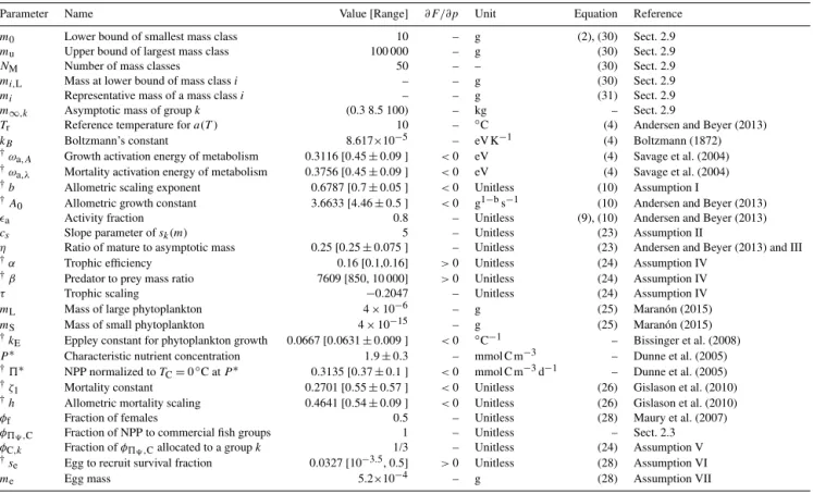
Table 1.Ecological model parameters. Assumption (I) (Brown et al., 2004; Savage et al., 2004; Andersen and Beyer, 2013); assumption (II) value of slope sufficiently large to have abrupt increase in allocation of reproduction from 0 to 1; assumption (III) (Beverton, 1992; Charnov
et al., 2012); assumption (IV) (Jennings et al., 2008; Barnes et al., 2010; Irigoien et al., 2014).βtruncated since we only consider fish up
to 100 kg; assumption (V) Equal partitioning of net primary production to each group; assumption (VI) (Dahlberg, 1979; Andersen and Pedersen, 2010; Pulkkinen et al., 2013). Assumption (VII) (Duarte and Alcaraz, 1989; Cury and Pauly, 2000; Freedman and Noakes, 2002;
Maury et al., 2007). The†symbol in the first column identifies parameters that were considered in the tuning procedure of the companion
paper (Carozza et al., 2016).∂F /∂pis the rate of change of equilibrium biomass (calculated over the three groups) with respect to change in
a parameterp.
Parameter Name Value [Range] ∂F /∂p Unit Equation Reference
m0 Lower bound of smallest mass class 10 – g (2), (30) Sect. 2.9
mu Upper bound of largest mass class 100 000 – g (30) Sect. 2.9
NM Number of mass classes 50 – – (30) Sect. 2.9
mi,L Mass at lower bound of mass classi – – g (30) Sect. 2.9
mi Representative mass of a mass classi – – g (31) Sect. 2.9
m∞,k Asymptotic mass of groupk (0.3 8.5 100) – kg – Sect. 2.9
Tr Reference temperature fora(T ) 10 – ◦C (4) Andersen and Beyer (2013)
kB Boltzmann’s constant 8.617×10⁻⁵ – eV K−1 (4) Boltzmann (1872)
†ω
a,A Growth activation energy of metabolism 0.3116 [0.45±0.09 ] <0 eV (4) Savage et al. (2004)
†ω
a,λ Mortality activation energy of metabolism 0.3756 [0.45±0.09 ] <0 eV (4) Savage et al. (2004)
†b Allometric scaling exponent 0.6787 [0.7±0.05 ] <0 Unitless (10) Assumption I
†A
0 Allometric growth constant 3.6633 [4.46±0.5 ] <0 g1−bs−1 (10) Andersen and Beyer (2013)
ǫa Activity fraction 0.8 – Unitless (9), (10) Andersen and Beyer (2013)
cs Slope parameter ofsk(m) 5 – Unitless (23) Assumption II
η Ratio of mature to asymptotic mass 0.25 [0.25±0.075 ] – Unitless (23) Andersen and Beyer (2013) and III
†α Trophic efficiency 0.16 [0.1,0.16] >0 Unitless (24) Assumption IV
†β Predator to prey mass ratio 7609 [850, 10 000] >0 Unitless (24) Assumption IV
τ Trophic scaling −0.2047 – Unitless (24) Assumption IV
mL Mass of large phytoplankton 4×10⁻⁶ – g (25) Maranón (2015)
mS Mass of small phytoplankton 4×10⁻¹⁵ – g (25) Maranón (2015)
†k
E Eppley constant for phytoplankton growth 0.0667 [0.0631±0.009 ] <0 ◦C−1 – Bissinger et al. (2008)
P∗ Characteristic nutrient concentration 1.9±0.3 – mmol C m−3 – Dunne et al. (2005)
†5∗ NPP normalized toT
C=0◦C atP∗ 0.3135 [0.37±0.1 ] <0 mmol C m−3d−1 – Dunne et al. (2005) †ζ
1 Mortality constant 0.2701 [0.55±0.57 ] <0 Unitless (26) Gislason et al. (2010)
†h Allometric mortality scaling 0.4641 [0.54±0.09 ] <0 Unitless (26) Gislason et al. (2010)
φf Fraction of females 0.5 – Unitless (28) Maury et al. (2007)
φ59,C Fraction of NPP to commercial fish groups 1 – Unitless – Sect. 2.3
φC,k Fraction ofφ59,Callocated to a groupk 1/3 – Unitless (24) Assumption V
†s
e Egg to recruit survival fraction 0.0327 [10−3.5, 0.5] >0 Unitless (28) Assumption VI
me Egg mass 5.2×10⁻⁴ – g (28) Assumption VII
is the growth constantA0(g1−bs−1) modulated by the van’t
Hoff–Arrhenius temperature dependence for growthaA(T ) (Eq. 4).
The energy input we wish to resolve is that for both growth and reproduction, and so we add the reproduction termkrm
to both sides of Eq. (9) to find the energy input to be
ξVB,k=Amb−kam. (10)
Although the interpretation of the terms in Eq. (10) do not exactly correspond to von Bertalanffy’s original interpreta-tion of a balance between anabolic growth and catabolic de-cay, we refer to this equation as the von Bertalanffy energy input ξVB,k. We consider different values of the activation energy of metabolism for growth ωa,A and mortalityωa,λ (Eq. 4), which result in different temperature dependence curves aA(T )andaλ(T ). The parameterb (unitless) is the allometric scaling constant, and ka (s−1) is the mass
spe-cific investment in activity. We follow Andersen and Beyer (2013) and define a new constant ǫa=ka/(ka+kr), which
when combined with the idea that there is zero growth at
the asymptotic massm∞,k (Munro and Pauly, 1983; Chen et al., 1992; Andersen and Beyer, 2013), allows us to express the mass specific investment in activity as ka=Aǫamb∞−,k1.
At each group’s asymptotic mass, we therefore have that
ξVB,k(m∞,k)=A(1−ǫa)mb∞,k.
Equation (7) for the input of energy to growth and repro-duction is therefore
ξI,k=min φ
C,kπ m
fk
, Amb−kam
, (11)
the minimum of a term that depends on biomass and one that does not. Applying the definition of the fish production spec-tra that we introduce in the next section (Eq. 24), we have a change in growth regime whenfkis such that
fk<
φC,k5ψ
mψ
mτ
Amb−k
am
. (12)
maximum physiological rate, and any unused energy avail-able to fish production is assumed to be transferred to unre-solved parts of the ecosystem. For low productivity systems, the model could overestimate biomass since a larger frac-tion of primary producfrac-tion will be transferred to commercial species. However, in high productivity systems, the allomet-ric limit is more likely to set growth rates; therefore a larger fraction will be transferred to the non-commercial groups. That said, the potential for, and the magnitude of, such a fea-ture will depend on the particular values of the growth rates at the site in question (Eq. 11).
2.4 Energy allocation to reproduction
We assume that the energy allocated to reproduction
γR,k(m, t )is proportional to the total input energyξI,k(m, t ) such that
γR,k=8kξI,k, (13)
where8k(m)is the mass-dependent fraction of input energy that is allocated to reproduction. From Eq. (6), we write the growth rate as
γS,k=(1−8k) ξI,k. (14)
We now derive an expression for 8k(m). Following Hartvig et al. (2011), we assume that the allocation to re-production is proportional to mass (Blueweiss et al., 1978; West et al., 2001; Lester et al., 2004; Andersen and Beyer, 2013), and that it also scales with a size-dependent ratesk(m) that defines the size-structure of the transition to maturity (Eq. 23). This gives us
γR,k=krmaxskm, (15)
where krmax is a normalizing constant. Combined with Eq. (13), we have that
γR,k=8kξI,k=kmaxr skm, (16)
whereξI,kis a representative input energy that we employ to guarantee that the allocation to reproduction does not change with biomass. For the representative input energy, we take the maximum possible value; that is, the von Bertalanffy input energy described in Eq. (10), and so have thatξI,k=ξVB,k. We therefore determine8k(m)for the energy input regime that is not limited by fish production, and find that
8k=
kmaxr skm
ξVB,k
. (17)
We determine krmax by applying the definition of the asymptotic mass, namely that it is the mass at which energy is only allocated to reproduction and so8k(m∞,k)=1. This gives
8k(m∞,k)=
krmaxsk(m∞,k)m∞,k
ξVB,k(m∞,k, t )
=1, (18)
and so we have that
kmaxr =ξVB,k(m∞,k, t )
sk(m∞,k)m∞,k
. (19)
We replace this value ofkrmaxinto Eq. (17) to find that
8k=
sk
sk(m∞,k)
m m∞,k
ξVB,k(m∞,k, t )
ξVB,k
. (20)
Applying Eq. (10) forξVB,k, and noting thatsk(m∞,k)is essentially equal to 1, we find that
8k=sk
1−ǫa
m/m∞,k
b−1 −ǫa
. (21)
Bringing this development together with Eq. (14), the in-dividual fish growth rate is
γS,k= 1−sk
1−ǫa
m/m∞,k
b−1 −ǫa
!
min
φC,kπ m
fk
, Amb−kam
. (22)
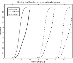
As in Hartvig et al. (2011), we assume that the mass struc-ture of the allocation of energy to reproduction sk(m) is a sharply transitioning function that shifts from near zero to near one around the mass of maturity mα,k. Based on Beverton (1992) and Charnov et al. (2012), we further as-sume that the mass of maturity is proportional to the asymp-totic massm∞,ksuch thatmα,k=ηm∞,k(Table 1). Although other functional forms are plausible,sk(m)must have a tran-sition in mass that is proportional tom∞,k(or to the maturity mass) (Hartvig et al., 2011), and so we use the functional form used by Hartvig et al. (2011),
sk= "
1+
m mα,k
−cs#−1
, (23)
where the parametercsdetermines how quickly the transition from zero to one takes place (Fig. 2). For reference, we cal-culate the reproduction allocation mass scale, the range over which the majority of the change in reproduction allocation takes place, as the inverse of the derivative evaluated at the maturity mass,(dsk
dm|m=mα,k)
−1, which we find to be 4mα,k
cs .
2.5 Fish production spectrum
Table 2.Ecological model variables.
Symbol Name Unit Equation
m Size (mass) of fish g –
t Time s –
T Temperature K or◦C –
f (m, t ) Fish biomass spectrum gwB m−2g−1 (1)
F (m, t ) Cumulative fish biomass gwB m−2 –
γS,k(m, t ) Individual fish growth rate g s−1 (22)
3k(m, t ) Natural mortality rate s−1 (1), (26)
a(T ) Van’t Hoff–Arrhenius temperature dependency Unitless (4)
ξI,k(m, t ) Total input energy to growth and reproduction g s−1 (11)
γR,k(m, t ) Energy allocated to reproduction g s−1 (13)
ξP,k(m, t ) Energy input from net primary production g s−1 (8)
ξVB,k(m, t ) Energy input from allometric theory g s−1 (10)
5(m, t ) Fish production gwB m−2s−1 (8)
π(m, t ) Fish production spectrum gwB m−2g−1s−1 (8), (24)
Nk(m, t ) Cumulative group abundance # m−2 (8), (A1)
nk(m, t ) Group abundance spectrum # m−2g−1 (8), (A1)
ka Mass specific investment in activity s−1 (10)
sk(m) Mass structure of energy to reproduction8(m) Unitless (23)
8k(m) Fraction of input energy to reproduction Unitless (21)
5ψ(t ) Net primary production mmol C m−3d−1 (24)
5ψ Annual average net primary production mmol C m−3d−1 (33)
mψ(t ) Representative mass of phytoplankton g (24), (25)
8L(t ) Fraction of large phytoplankton production Unitless (25)
RP(m0, t ) Primary-production-determined recruitment gwB m−2s−1 (27)
Re,k(m0, t ) Egg production and survival determined recruitment gwB m−2s−1 (28)
Rk(m0, t ) Overall recruitment gwB m−2s−1 (29)
1.5 2 2.5 3 3.5 4 4.5
0 0.1 0.2 0.3 0.4 0.5 0.6 0.7 0.8 0.9 1
Scaling and fraction to reproduction by group
Mass (log10 g)
Fraction
Small Medium Large
Figure 2. Mass dependence of reproduction by group. The mass
scaling functionsk(m)(thin lines, Eq. 23) determines the mass
de-pendence of the allocation of energy to reproduction.8k(m)(thick
lines, Eq. 21) is the fraction of energy allocated to reproduction.
(mmol C m−2g−1s−1). Following Brown et al. (2004) and Jennings et al. (2008), we base this formulation on (1) the NPP5ψ(t )(mmol C m−2s−1) (Sect. 2.8), (2) the representa-tive size at which NPP takes placemψ(t )(g) (Jennings et al.,
2008), and (3) the trophic scaling exponentτ that indicates how efficiently energy is transferred through the trophic web, whereτdepends on the trophic efficiencyαand the predator to prey mass ratioβ, and is equal to log(α)/log(β)(Brown et al., 2004). The fish production spectrum follows
π=5ψ
mψ
m
mψ
τ−1
. (24)
As in Brown et al. (2004), we assume thatαandβ, and henceτ, are constant. From the expression for fish produc-tion detailed in Eq. (24), we determine the individual fish growth rate using Eq. (22).
πk for largemand overestimateπkfor smallm. Essentially, a mass-dependent β would tend to decrease the steepness of biomass spectra relative to what is shown here. It is also commonly assumed that the trophic efficiencyαis constant (Brown et al., 2004; Jennings et al., 2008; Tremblay-Boyer et al., 2011). Based on acoustic biomass estimates and mod-elling work, Irigoien et al. (2014) suggests that trophic effi-ciency can instead be significantly different in low and high productivity regions, at different levels in the food web (from phytoplankton to mesozooplankton and from mesozooplank-ton to fish) and that it can also depend on environmental pa-rameters such as temperature (through its influence on organ-ismal metabolic rates) and water clarity (which affects visual predation). Quantifying variability inτ is an important target for future work.
The production spectrum is the product of two terms. The first is the initial value determined at the representative phy-toplankton massmψ(t ), which corresponds to the NPP nor-malized by the representative phytoplankton size. The fish production spectrum then follows a power law dependence in m with a scaling exponent of τ−1. This mass scaling represents larger phytoplankton (largermψ(t )) being trophi-cally closer to fish than smaller phytoplankton, thereby per-mitting more energy to be transferred from phytoplankton to fish (Ryther, 1969). The power law dependence that we use is based on Kooijmann (2000) and Brown et al. (2004). The model is forced with observations of NPP, and so we run the model in units of mmol C. For analysis and presentation, we convert to grams of wet biomass (gwB) by assuming that there are 12 g C per mol C, and that there are 10 gwB for ev-ery g of dry carbon (Jennings et al., 2008).
Phytoplankton mass ranges over several orders of magni-tude (Jennings et al., 2008). We take a simple approach and express the spectrum of phytoplankton as a single represen-tative mass at which NPP takes place. Due to the wide range of phytoplankton mass, we calculate the representative mass as
mψ=m8LL(t )m 1−8L(t )
S , (25)
and so take the geometric mean of the mass of a typical large,
mL, and a typical small,mS, phytoplankton, weighted by the
fraction of production due to large or small phytoplankton,
8L(t )and 1−8L(t ), respectively. We calculate this fraction
using the phytoplankton size structure model of Dunne et al. (2005), which resolves small and large phytoplankton and assumes that small zooplankton are able to successfully prey upon increasing production of small phytoplankton, but that large zooplankton are unable to do so as effectively for large phytoplankton production. Dunne et al. (2005) propose an empirical relationship for the large fraction of NPP8L(t )in
terms of temperatureTC(t )(◦C) and the NPP, the Eppley
fac-torekETC(t )wherek
E(◦C−1) is the Eppley temperature
con-stant for phytoplankton growth, and 5∗ (mmol C m−3d−1) the productivity normalized to a temperature of 0◦C. The
Dunne et al. (2005) model resolves a high fraction of the vari-ability in phytoplankton community structure (Agawin et al., 2000), and provides a mechanism to explain how the frac-tion of large phytoplankton biomass increases with increas-ing phytoplankton biomass. Although we use this particular formulation for the large fraction in Eq. (25), future work could examine alternatives (Denman and Pena, 2002). 2.6 Natural mortality
The natural mortality term represents all forms of natural (non-fishing) mortality. It mainly consists of predation, but also includes non-predatory sources of mortality such as par-asitism, disease, and senescence (Pauly, 1980). This term is of first-order importance in determining energy flows in ma-rine food webs, and so also in determining biomass. In pursu-ing our principle of uspursu-ing empirical parameterizations to rep-resent complex processes that are incompletely understood, we follow the work of Gislason et al. (2010) and Charnov et al. (2012) and take the mortality rate to be
3k=λm−hmh∞+,kb−1, (26)
where λ=eζ1(A
0/3)aλ(T ) (see Appendix B for a full derivation of this form).ζ1 is a parameter estimated from
mortality data (Gislason et al., 2010), A0 (g1−bs−1) is the
growth constant from Eq. (10), andaλ(T )is the van’t Hoff– Arrhenius exponential for mortality as described in Eq. (4). Charnov et al. (2012) provided a mechanistic underpinning for Eq. (26) by calculating the optimal number of daughters per reproducing female over that female’s lifetime. Unlike other empirical mortality rate frameworks, such as that of Savage et al. (2004), the mass dependencem−hdoes not de-pend on the allometric growth scaling b, and so the mass dependence of the mortality rate is not determined by inter-nal biological parameters, but by predation and competition (Charnov et al., 2012). The losses due to natural mortality, term 3 in Eq. (1), are linearly proportional to biomass as in Gislason et al. (2010), and in keeping with the classical MVF model.
Since the prey mortality rate does not depend on the preda-tor biomass, we do not resolve top-down trophic cascades (Andersen and Pedersen, 2010; Hessen and Kaartvedt, 2014). At present, a scarcity of data hinders a formal verification of generalized trophic cascades in the open ocean, which would be desirable for the formulation of their impact within the BOATS framework. However, we do represent bottom-up ef-fects through the growth formulation described in Eq. (1), since a change in biomass in one size class is carried upward through the trophic web as fish grow to larger mass classes.
2.7 From reproduction to recruitment
Fish reproduction and recruitment comprise a set of com-plex ecological processes that result in new fish biomass en-tering a fishery (Myers, 2002). This first involves fish allo-cating energy to reproduction and releasing eggs and sperm during spawning. Fertilized eggs must then survive preda-tion until they hatch to become larvae, when they must again survive predation until they grow into juveniles (Dahlberg, 1979; McGurk, 1986; Myers, 2001). The end of the juvenile stage is generally defined as when fish reach sexual maturity or when they begin interacting with other adult members of the fishery (Kendall et al., 1984). The definition of a recruit is more nuanced since it generally depends on the fishery in question and can be based on a particular size or age, the size or age of sexual maturity, or the size or age at which fish can be caught (Myers, 2002). For the model, we refer to re-cruitment as the flux of new biomass into the lower boundary mass (m0) of each group.
Recruitment is driven by biomass-dependent (density-dependent) processes, such as predation and disease, as well as by biomass-independent (density-independent) processes such as environmental change. These processes strongly and nonlinearly affect mortality throughout the egg, larval, and juvenile stages (Dahlberg, 1979; McGurk, 1986; My-ers, 2002). To model the number of recruits that result from a given spawning stock of biomass, one must make assump-tions on the nature of these processes. The widely used stock-recruitment models of Ricker (1954), Schaefer (1954), and Beverton and Holt (1957), and the generalization of these models by Deriso (1980) and Schnute (1985), make such assumptions and operate in terms of the spawning stock biomass; that is, the biomass that is of reproductive age.
We model recruitment by considering both the NPP and the production and survival of eggs by adult fish. Our formu-lation is based on the Beverton–Holt stock recruitment rela-tionship (which employs a Holling Type 2 functional form, Holling, 1959), as used by Beverton and Holt (1957) and An-dersen and Beyer (2013), with NPP setting the upper limit and the half-saturation constant (Eq. 29). This form allows for an approximately linear decrease to zero recruitment as the spawning stock biomass goes to zero, but sets an up-per limit that depends on the NPP when the spawning stock
biomass is large, in order to represent the role of food avail-ability in determining larval survival.
The flux of biomass out of a mass class is the growth rate multiplied by the biomass in that mass class (Eq. 1). Since the recruitment is also a flux of biomass (one that occurs at the lower mass boundary), to define it in terms of NPP
RP,k(m0, t )(gwB m−2s−1), we apply Eq. (8) and find that
RP,k(m0, t )=γP,k(m0, t )fk(m0, t )
=φC,kπ(m0, t )m0
fk(m0, t )
fk(m0, t )
=φC,kπ(m0, t )m0, (27)
wherem0is the lower bound of the smallest mass class, and
π is the fish production spectrum from Eq. (24). Alterna-tively, the recruitment from the production and survival of eggs to recruits,Re,k(m0, t )(gwB m−2s−1), depends on the
energy allocated to reproduction,γR,k(t )(Eq. 13), by allnk individuals over all mass classes, which we write as
Re,k(m0, t )=φfse
m0
me m∞,k
Z
m0
γR,knkdm. (28)
The model biomass includes both males and females, which are assumed to mature at the same mass (Beverton, 1992). As in other model studies (Maury et al., 2007; Ander-sen and PederAnder-sen, 2010; AnderAnder-sen and Beyer, 2013), males and females of reproductive age continually reproduce, yet only the female contribution is counted in the flux into the smallest mass class, since the male contribution to a fertil-ized egg is negligible compared to that of the female. Hence, when the integral part of Eq. (28) is multiplied by the frac-tion of females,φf, we have the biomass of eggs produced.
Dividing by the mass of an eggmetherefore gives the
num-ber of eggs produced, which when multiplied by the survival fractionse, expressing the probability that an egg becomes
a recruit, gives the number of recruits. From the number of recruits produced per unit time, we multiply by the mass of a recruit,m0, to determine the biomass flux of recruits.
Applying the same form as the stock-recruitment model developed by Beverton and Holt (1957) (see Andersen and Beyer, 2013) we take the overall recruitment Rk(m0, t )
(gwB m−2s−1) to be
Rk(m0, t )=RP,k(m0, t )
Re,k(m0, t )
RP,k(m0, t )+Re,k(m0, t )
. (29)
Following Andersen and Beyer (2013), we take the half-saturation constant (the value of Re,k(m0, t ) at which the
overall recruitment is one half of the maximum recruit-ment allowed by productivity) to be RP,k(m0, t ). Figure 3
shows how the overall recruitment Rk(m0, t ) changes as
a function ofRP,k(m0, t )andRe,k(m0, t ). As is the case for
R P (gwB m
−2 yr−1)
Re
(gwB m
−2
yr
−1
)
Recruitment flux
5
5
5
5 5
10
10
10
10
15
15
15
20
20
20
25
25
0 5 10 15 20 25 30
0 50 100 150 200 250 300
0 5 10 15 20 25 30
Figure 3. Recruitment flux. The recruitment flux of group k,
Rk(m0, t )(gwB m−2yr−1, Eq. 29) as a function of the recruitment
based on the boundary flux of NPPRP,k(m0, t )(gwB m−2yr−1,
Eq. 27), and the recruitment from production and survival of eggs
Re,k(m0, t )(gwB m−2yr−1, Eq. 28).
also the egg- and survival-based recruitmentRe,k(m0, t )
in-creases, the overall recruitment saturates toward the primary production-based limit RP,k(m0, t ). This indicates that for
sites with high biomass, NPP limits recruitment. At the other extreme, when Re,k(m0, t ) is small relative to RP,k(m0, t ),
the recruitment is approximately linear in Re,k(m0, t ) and
so has a weak dependence onRP,k(m0, t )such that at low
biomass the egg production and survival limits recruitment. Tables 1 and 2 detail the fish model parameters and vari-ables, respectively. The group and mass class structure, and the numerical discretization of the continuous biomass spec-tra, are presented in Sect. 2.9 and Sect. 2.10, respectively. 2.8 Environmental forcing: temperature and net
primary production
The ecological model requires temperature and NPP infor-mation as forcing input to calculate the time evolution of biomass (Eq. 1). These variables can be provided by an ocean general circulation model that includes a lower trophic level model. Here, we instead use observational estimates, which would be expected to provide a more realistic simulation. For temperature, we use the World Ocean Atlas 2005 (Locarnini et al., 2006), which brings together multiple sources of in situ quality-controlled temperature interpolated to monthly climatologies on a 1◦×1◦grid. We discuss our usage of
tem-perature in Sect. 2.2, and as discussed above, use the aver-age water temperature from the upper 75 m of the water col-umn to force temperature-dependent rates. For NPP, we take the average of three satellite-based estimates (Behrenfeld and Falkowski, 1997; Carr et al., 2006; Marra et al., 2007) to cap-ture some of the variability that exists in different NPP mod-els (Saba et al., 2011). We note that satellite-based estimates suffer from a range of shortcomings, including lack of
pro-ductivity sources other than phytoplankton (e.g. seagrass and corals), and biases in coastal regions and estuaries (Smyth, 2005; Saba et al., 2011). Although overall minor (see Cross-land et al., 1991; Duarte and Chiscano, 1999), these uncer-tainties will carry through to the modelled biomass and har-vest.
2.9 Group and mass class structure
Fish span several orders of magnitude in mass, and we therefore discretize the mass spectra into logarithmic mass classes. In order to directly compare our results with the Sea Around Us Project (SAUP) harvest database (Watson et al., 2004; Pauly, 2007), we consider three fish groups each with a different asymptotic mass. We first convert the maximum lengths used in the SAUP (30 cm for the small group, 90 cm for medium group, and up to our maximum resolved length for the large group) to asymptotic length assuming that the maximum length is 95 % of the asymp-totic length (Taylor, 1958; Froese and Pauly, 2014), and then apply a length–weight relationship of the form m=δ1lδ2
(Froese et al., 2013) to calculate the asymptotic mass. This results in asymptotic masses of 0.3, 8.5, and 100 kg for the small, medium, and large groups, respectively.
Although the asymptotic masses differ, all three groups have the same mass class structure, with lower and upper bounds ofm0 = 10 g andmu = 100 kg, respectively. Since
the groups have different asymptotic massesmk,∞, there are
therefore fewer resolved mass classes for groups with smaller asymptotic mass. We define the mass classes by dividing the mass spectrum intoNMclasses with lower boundsmi,Lsuch
that
mi,L=m0
mu
m0
i−1
NM
, (30)
whereiis the index of the mass class that ranges from 1 to
NM. Based on this definition, we describe a mass class as an
intervalIi= [mi,L, mi+1,L]of length1mi =mi+1,L−mi,L
(i=1, . . ., NM). We divide the spectrum into 50 mass classes
(NM=50). Although we use fewer mass classes than some
other studies (Maury et al., 2007; Hartvig et al., 2011), we have tested higher temporal and spatial resolutions and find that our interpretations would not be influenced by our choice of temporal or spatial resolution.
When we calculate and present mass-dependent quantities, we consider a massmi that represents the average or central value of its class. For this, we apply the geometric mean of the lower and upper bounds of a mass class, which we calcu-late as
mi = mi,Lmi+1,L1/2, (31)
2.10 Numerical methods
The biological part of our model is a system of three non-linear first-order (in mass) partial differential equations that describe the evolution of the biomass spectra of three fish groups. Each equation is forced with the same net primary production and temperature information, and the equations do not interact with one another. Here, we use the standard notation of a subscriptito describe a mass cell, and a super-scriptnto describe a temporal cell. The notationk, as in the main text, refers to a fish group. For example,fk,in+1 repre-sents the biomass spectral valuef of groupk, at mass class
iat timen+1.
Since the McKendrick von-Foerster model is an advec-tive equation in biomass, as is true of advecadvec-tive equations, transport errors are a concern (Press et al., 1992). To limit such errors, and because growth is always defined to be pos-itive (or zero), we apply an upwind scheme (Maury et al., 2007; Hartvig et al., 2011). This numerical scheme uses only biomass information that is upwind of the cell of interest; that is, it only uses biomass information at cellsiandi−1 to integrate and determine the biomass at celli at the next timestep. We use a forward difference scheme for the tempo-ral rate of change, and explicitly calculate the growth (γ) and mortality (3) rates; that is, we use the current temporal state of biomass fk,in to update the biomass, as opposed to using the future biomass statefk,in+1as in an implicit scheme, and integrate biomass as
fk,in+1=fk,in +
−
γn
k,ifk,in −γk,in−1fk,in−1
1mi
+γ n k,if
n k,i
mi
−3nk,ifk,in
1t. (32)
The model is stable and converges as we decrease1t.
3 Results and discussion
Here we describe the behaviour of the fish ecology model, and make use of a simplified version of the model as a ref-erence point and initial biomass condition. We consider two model grid points that correspond to individual patches of ocean at a cold-water site in the East Bering Sea (EBS) LME (64◦N, 165◦W) and a warm-water site in the Benguela
Current (BC) LME (20◦S, 12◦E), and describe the
result-ing biomass spectra and other model variables. We discuss the results from a sensitivity test that considers the role of NPP (ranging from 50 to 2000 mg C m−2d−1) and tempera-ture (ranging from−2 to 30◦C) on biomass. For these sim-ulations, we use a 15 day timestep and constant forcing of annually averaged NPP and temperature.
We do not use these sites for a thorough data-based model validation, which is difficult at this time due to a lack of suitable fish biomass data. The parameter values used here
1 2 3 4 5
−3 −2 −1 0 1 2
(a) Cold−water site f k
Mass (log10 g)
Spectra (log10 gwB m
−2
g
−1
)
Small
Medium
Large
Total
1 2 3 4 5
−3 −2 −1 0 1 2
(b) Warm−water site f k
Mass (log10 g)
Figure 4.Steady state biomass spectra at two sites. Black solid, dashed, and dash–dot curves represent the small, medium, and large group biomass, respectively, whereas the grey curves represent the total of the three groups. The model is forced at two sites with
an-nual average net primary production (NPP) and temperature (T)
with a timestep of 15 days. Simulations are for a(a)cold-water site
in the East Bering Sea LME (64◦N, 165◦W) and a(b)warm-water
site in the Benguela Current LME site (20◦S, 12◦E).
are taken from an extensive data-model comparison that em-ploys the global implementation of the model, and is fully described in the companion paper (Carozza et al., 2016). In that study, we take a Monte Carlo approach with over 10 000 parameter sets to find parameter combinations that best fit observed harvest at the LME-scale, considering the full range of the uncertain parameter space for the 13 most important parameters. Of these 13 parameters, 2 are eco-nomic, with the remaining 11 ecological parameters being identified with a dagger symbol in Table 1. Beyond the val-idation to harvest at the LME-scale in the companion paper, more specific validation could be done in the future with suit-able data sets when they become availsuit-able (that is, size ag-gregated, regional-scale, species-comprehensive biomass as-sessments).
3.1 Initial biomass state
To begin our results and analysis section, we make a series of simplifying assumptions in order to derive an analytical biomass spectrumfk,m,0, which we use as a reference point
for evaluating aspects of the full model. Since this analyti-cal biomass state is a reasonable approximation of the full model, we also use it as an initial biomass condition for our simulations.
Beginning with the evolution of biomass in Eq. (1), we assume that the input energy expressed in Eq. (7) is solely controlled by NPP, so that ξI,k(m, t )=ξP,k(m, t )=
φC,kπ(m, t )m/fk(m, t ), and that there is no allocation
of energy to reproduction, so that 8k(m)=0. These two assumptions result in a growth rate of γS,k(m, t )=
φC,kπ(m, t )m/fk(m, t ), which allows us to calculate the
in the mortality rateλand representative phytoplankton mass
mψterms), and find that the equilibrium biomass spectrum of each each group is
fk,m,0=
φC,k5ψ(1−τ )
λmτψmh∞+,kb−1 m
τ+h−1.
(33)
As expected from the MVF model, biomass follows a power law spectrum with respect to mass. Given that the power law scaling exponent isτ+h−1, biomass scales as a function of the trophic and mortality scalings, which we assume are constant. On the other hand, the intercept of the spectrum (in logarithmic space, when m=m0=10 g)
de-pends on a variety of parameters such as the NPP and trophic efficiency, as well as the natural mortality rate and the rep-resentative phytoplankton mass. Unlike the mass scaling, the intercept is also group dependent through the fraction of pri-mary production allocated to each group and the asymptotic mass.
3.2 Biomass equilibrium
As in other studies, we use features of the modelled biomass spectra, shown in Fig. 4, to interpret the model results. Work on marine ecosystems indicates that biomass spectra, when plotted in log-log space, are approximately linear over most of the size range and have slopes that range from −1.0 to
−1.2 (Blueweiss et al., 1978; Brown et al., 2004; Marquet et al., 2005; White et al., 2007). Ignoring harvest, group biomass spectra generally decrease with size, except at the maturity mass at which energy begins to be allocated to re-production (Fig. 2), where there is a decrease in the growth rate and thereby an accumulation of biomass that may result in a local maximum or a local decrease of the spectrum slope (Andersen and Beyer, 2013). As expected from Eq. (33), the group intercepts differ, but only by little since in our formu-lation the only difference arises from the weak asymptotic mass dependencemh∞+,kb−1in the mortality term. Biomass is larger at the cold-water site, despite it having a lower NPP (Fig. 5). In particular, large group biomass is larger at the cold-water site, which is consistent with the findings of Wat-son et al. (2014).
There is a nonlinear decrease in biomass at larger mass classes (Fig. 4). The shape of the biomass spectra are deter-mined from the growth and mortality rates. Since the growth rate consists of NPP and allometric regimes (Eq. 22), and the mortality rate of a single regime (Eq. 26), any changes in the shape of the biomass spectra are determined by the growth rate. We generally find that the NPP regime (Eq. 8) limits energy input in smaller mass classes, whereas the allometric regime (Eq. 10) plays the limiting role in the largest mass classes.
Temperature (oC)
NPP (mg C m
−2
d
−1)
(a) Total biomass (log10 gwB m−2)
0 0.5
1
1.5
2
2 2.5 3
0 10 20 30
500 1000 1500 2000
−0.5 0 0.5 1 1.5 2 2.5 3 3.5
Temperature (oC)
NPP (mg C m
−2
d
−1)
(b) Intercept of total biomass spectra (log10 gwB m−2g−1)
−1 −0.5
0 0.5
1
1 1.5
0 10 20 30
500 1000 1500 2000
−1.5 −1 −0.5 0 0.5 1 1.5 2
0 10 20 30
−1.1 −1 −0.9 −0.8 −0.7 −0.6
Temperature (oC)
Slope (log10 gwB m
−2g −1/log10 g)
(c) Slope of nonreproducing biomass spectra
Small Medium
Large Total
Figure 5.Model sensitivity to net primary production (NPP) and
temperature (T).(a)Total biomass in terms of NPP andT,(b)
in-tercept of total fish spectrum in terms of NPP andT, and(c)group
and total slope of the non-reproducing part of the fish biomass
spec-tra. In(c), since the slopes of the biomass spectra do not depend on
NPP, the slopes are lines that depend only on temperature. Red and
blue circles in(a)and(b)represent the NPP andT of the warm- and
cold-water sites, respectively, used in Fig. 4. All total spectral inter-cepts and slopes are calculated by adding the biomass in each mass class over all three groups. The intercept is the spectral biomass of the first mass class, and the slope is calculated from the mass classes
that are smaller than the maturity massmα,k(the non-reproducing
mass classes).
3.3 Sensitivity tests
Total biomass (Fig. 5a) increases monotonically for increas-ing NPP, yet decreases monotonically for increasincreas-ing temper-ature. Increasing temperature not only reduces the primary-production-based growth rateγPby reducing the
representa-tive phytoplankton size (Eq. 24), it also significantly drives up the mortality rate, generating a clear pattern of reduced biomass. Under the allometric regime of growth (Eq. 10), higher temperature implies a greater growth rate, which on its own results in an increase in biomass (not shown). How-ever, this feature is more than counterbalanced by the mor-tality rate increase, which results in an overall lower biomass for higher temperature.
nonlin-early changing in temperature due to the multiple sources of temperature dependence in the intercept (Eq. 33). The biomass slope does not depend on NPP (Fig. 5c), as indicated in Eq. (33), and the resulting total slope values (grey curve in Fig. 5c), given the parameters used in this single realiza-tion of the model, are consistent with published values from marine ecosystems that range from−1.0 to−1.2 (Blueweiss et al., 1978; Brown et al., 2004; Marquet et al., 2005; White et al., 2007). However, we find flatter slopes for lower tem-peratures, to values as low as −0.9. This implies that our model would result in generally higher biomass than if the slope of the spectra fell between−1 and−1.2. Equation (33) also indicates that the slope is not a function of tempera-ture. That equation applies for the small group (blue curve in Fig. 5c) over all temperatures, and for the medium group at low temperatures. However, when the input energy is de-termined by the von Bertalanffy limit, as is the case for high temperatures in the medium group and all temperatures for the large group, a rise in temperature steepens the biomass slope. Overall, NPP only influences spectra by shifting the intercept, whereas temperature both shifts the intercept and changes the slopes of biomass spectra when the input energy is set by the von Bertalanffy limit.
The model illustrates hypothetical inferences, based on the macroecological theory it uses, that need to be compared to suitable observations. Further validation of the model at spe-cific locations and at the size-class level of detail remains a challenge because of the scarcity of suitable data sets. To further validate BOATS and comparable models, we require size-class-resolved observations at the ecosystem level, at a high enough resolution to detect variations in spectral prop-erties, and at a sufficient number of sites so as to detect bulk variations due to different temperature and NPP. This type of detail at the ecosystem level is not available even in current stock assessment databases, and it should be considered an important target for future data syntheses.
4 Conclusions
We have described a new marine upper trophic level model for use in gridded, global ocean models. The model as de-scribed here is used as the ecological module of the BOATS model, designed to study the global fishery. In a compan-ion paper, we discuss the economic module of the BOATS model and complete the model evaluation by comparing harvest simulations to global harvest observations. The ap-proach could be readily adapted to other purposes, such as for use in studies of ocean biogeochemistry or ecology.
The model uses NPP and temperature to represent the first-order features of fish biomass using fundamental marine bio-geochemical and ecological concepts. When possible, we ap-ply empirical relationships with mechanistic underpinnings to simplify complex ecological processes that are difficult to constrain. Phytoplankton community structure is represented by the proportion of large phytoplankton. Fish growth rates are determined by a parameterized trophic transfer of energy from primary production, but limited by empirical allometric estimates. The natural mortality rate is based on an empir-ical relationship that depends on the individual and asymp-totic mass, and reproduction depends on the NPP and the fish biomass of reproductive age. The resulting biomass spectra, as defined here, include all commercially harvested organ-isms longer than 10 cm (greater than 10 g).
We presented simulated biomass spectra at a warm- and a cold-water site, and performed a sensitivity test of the model forcing variables to examine key model variables. We find that the structure of modelled biomass spectra is broadly consistent with observations, and biomass slopes match ob-servations over a wide range of NPP and temperature. Al-though the model employs a limited number of parameters compared to similar modelling efforts, it retains reasonably realistic representations of biological and ecological pro-cesses, and is computationally efficient, which allows for ex-tensive sensitivity studies and parameter-space analyses even when implemented globally. Due to its dynamical generality and conceptual simplicity, the ecological module of BOATS is well-suited for global-scale studies where the resolution of species or functional-groups is not necessary.
Code availability