❊♥s❛✐♦s ❊❝♦♥ô♠✐❝♦s
❊s❝♦❧❛ ❞❡
Pós✲●r❛❞✉❛çã♦
❡♠ ❊❝♦♥♦♠✐❛
❞❛ ❋✉♥❞❛çã♦
●❡t✉❧✐♦ ❱❛r❣❛s
◆◦ ✹✸✹ ■❙❙◆ ✵✶✵✹✲✽✾✶✵
❋✐♥❞✐♥❣ ❛ ▼❛①✐♠✉♠ ❙❦❡✇♥❡ss P♦rt❢♦❧✐♦ ✲ ❆
●❡♥❡r❛❧ ❙♦❧✉t✐♦♥ t♦ ❚❤r❡❡✲▼♦♠❡♥ts P♦rt❢♦✲
❧✐♦ ❈❤♦✐❝❡
●✉st❛✈♦ ▼✳ ❞❡ ❆t❤❛②❞❡✱ ❘❡♥❛t♦ ●❛❧✈ã♦ ❋❧ôr❡s ❏✉♥✐♦r
❙❡t❡♠❜r♦ ❞❡ ✷✵✵✶
❖s ❛rt✐❣♦s ♣✉❜❧✐❝❛❞♦s sã♦ ❞❡ ✐♥t❡✐r❛ r❡s♣♦♥s❛❜✐❧✐❞❛❞❡ ❞❡ s❡✉s ❛✉t♦r❡s✳ ❆s
♦♣✐♥✐õ❡s ♥❡❧❡s ❡♠✐t✐❞❛s ♥ã♦ ❡①♣r✐♠❡♠✱ ♥❡❝❡ss❛r✐❛♠❡♥t❡✱ ♦ ♣♦♥t♦ ❞❡ ✈✐st❛ ❞❛
❋✉♥❞❛çã♦ ●❡t✉❧✐♦ ❱❛r❣❛s✳
❊❙❈❖▲❆ ❉❊ PÓ❙✲●❘❆❉❯❆➬➹❖ ❊▼ ❊❈❖◆❖▼■❆ ❉✐r❡t♦r ●❡r❛❧✿ ❘❡♥❛t♦ ❋r❛❣❡❧❧✐ ❈❛r❞♦s♦
❉✐r❡t♦r ❞❡ ❊♥s✐♥♦✿ ▲✉✐s ❍❡♥r✐q✉❡ ❇❡rt♦❧✐♥♦ ❇r❛✐❞♦ ❉✐r❡t♦r ❞❡ P❡sq✉✐s❛✿ ❏♦ã♦ ❱✐❝t♦r ■ss❧❡r
❉✐r❡t♦r ❞❡ P✉❜❧✐❝❛çõ❡s ❈✐❡♥tí✜❝❛s✿ ❘✐❝❛r❞♦ ❞❡ ❖❧✐✈❡✐r❛ ❈❛✈❛❧❝❛♥t✐
▼✳ ❞❡ ❆t❤❛②❞❡✱ ●✉st❛✈♦
❋✐♥❞✐♥❣ ❛ ▼❛①✐♠✉♠ ❙❦❡✇♥❡ss P♦rt❢♦❧✐♦ ✲ ❆ ●❡♥❡r❛❧ ❙♦❧✉t✐♦♥ t♦ ❚❤r❡❡✲▼♦♠❡♥ts P♦rt❢♦❧✐♦ ❈❤♦✐❝❡✴
●✉st❛✈♦ ▼✳ ❞❡ ❆t❤❛②❞❡✱ ❘❡♥❛t♦ ●❛❧✈ã♦ ❋❧ôr❡s ❏✉♥✐♦r ✕ ❘✐♦ ❞❡ ❏❛♥❡✐r♦ ✿ ❋●❱✱❊P●❊✱ ✷✵✶✵
✭❊♥s❛✐♦s ❊❝♦♥ô♠✐❝♦s❀ ✹✸✹✮ ■♥❝❧✉✐ ❜✐❜❧✐♦❣r❛❢✐❛✳
Finding a maximum skewness portfolio – a general solution to
three-moments portfolio choice
Gustavo M. de Athayde a , Renato G. Flôres Jr b, *
a
Banco Itaú, Rua Boa Vista 176, São Paulo 01014-919, Brazil
b
Escola de Pós-Graduação em Economia / Fundação Getulio Vargas, Praia de
Botafogo 190, 11° andar, Rio de Janeiro 22253-900, Brazil
______________________________________________________________________
Abstract
Considering the three first moments and allowing short sales, the efficient portfolios set for n risky assets and a riskless one is found, supposing that agents like odd moments and dislike even ones. Analytical formulas for the solution surface are obtained and important geometric properties provide insights on its shape in the three dimensional space defined by the moments. A special duality result is needed and proved. The methodology is general, comprising situations in which, for instance, the investor trades a negative skewness for a higher expected return. Computation of the optimum portfolio weights is feasible in most cases.
JEL classification: C49; C61; C63; G11
Keywords: Duality; Efficient set; Higher moments; Portfolio choice; Skewness.
______________________________________________________________________
(This version: September, 10; 2001)
* Corresponding author. Tel.: + 55-21-2559 5909; fax: + 55-21-2553 8822. E-mail address: [email protected] .
1. Introduction
Since at least Mandelbrot (1963)’s, economists and practitioners as well have been
aware that the distribution of asset returns very seldom is normal. In spite of the
considerable empirical literature now taking into account this fact (e.g. Campbell et al.,
1997), financial theory has been reluctant in incorporating higher order moments in its
developments. Portfolio choice – a most important subject for applications -, in spite of
pioneer contributions like Samuelson (1967) and Kraus and Litzenberger (1976), still is
largely dominated by the Markowitz Weltamschaung. In this paper we build up the
efficient portfolios set for the case in which consideration is given to the three first
moments. Ingersoll (1975), in an early effort in this direction, provided a clue on the
shape of a portfolio frontier with the first three moments. Nevertheless his solution was
based on differentiation of the utility function, and not on the technical constraints of
the efficient set.
We provide the characteristics and the shape of the efficient set, as well as ways
to assure the investor he is on it. Characterisation of the efficient set – i.e., the set of
points where one can’t get any better in any moment, without getting worse on another -
seems a much more plausible and feasible approach if interest lies in actual
computations related to practical problems as asset allocation, fund managing and
dynamic portfolio optimisation. In practice, use of criteria based on utility functions
may not seem reasonable for fund managers, especially those who need to report to their
clients the criteria used to select the portfolios.
In general, investors will prefer high values for odd moments and low ones for
even moments. The former can be seen as a way to decrease extreme values on the side
of losses and increase them on the gains’. The latter can be justified by the fact that even
moments measure dispersion, and therefore volatility; something undesirable because it
increases the uncertainty of returns. If the investor is focussed on the worst scenario,
like the Value at Risk of his portfolio, this kind of behaviour becomes even clearer and
more justifiable.
Based on the assumption that agents like odd moments and dislike even ones, we
shall build up the efficient portfolio frontier in the case of n risky assets and a riskless
one, considering the three first moments and allowing short sales. The resulting surface
will be represented in a convenient three dimensional space, whose co-ordinates are in
deviations (the square root of variance). Given the assumption at stake, we shall in
principle work in the positive orthant of R3 related to positive values in the three axes.
There might however be cases where, for instance, the investor will be either obliged or
open to trade a negative skewness for a higher expected return. Such situations are
comprised in our methodology, and many of the results are presented in the half-space
of R3, defined by the non-negativity constraint on the standard deviation.
The characterisation of the optimal surface will allow the actual computation of
optimum weights in most practical cases. All results suppose the existence of the
optimum, in the different optimisation programmes, what cannot be valid in certain
pathological situations which are not considered in the paper.
It is interesting to see the optimal surface as the set of points giving the highest
skewness for given mean and variance, but – as will be shown – they also give the
highest mean for given variance and skewness, and the lowest variance for a given
mean and skewness. In fact, it seems easier to attack the problem from this last
viewpoint.
The next section develops a few preliminaries necessary for obtaining the
results. They comprise a convenient notation and a duality proposition needed to pass
from one “three-moments programme” to another. Section three then studies the
efficient set for the minimum variance problem with given mean and skewness, while
section four develops some insightful examples. With the help of the duality result, in
section five we solve the complete problem. A final section concludes.
2. Preliminaries: notation and duality
2.1 A convenient notation
Dealing with higher moments can easily become algebraically cumbersome or
even intractable. Given a n-dimensional random vector, its moments can be seen as
tensors, a mathematical object well known to physicists, for instance. The second
moments tensor is the popular nxn covariance matrix, while the third moments one can
be visualised as a nxnxn cube in three-dimensional space. As with the covariance
number of different skewnesses is equal to that of combinations with repetition of three
elements out of n,
ö ç ç
è æ +
3 2
n
, and not n3 .
We shall transform the skewness tensor into a nxn2matrix by slicing each nxn
layer and pasting them, in the same order, sideways. The fact that one ends up with a
matrix allows the use of matrix differential calculus in all expressions and the derivation
of compact and elegant formulas. Calling σijk a general (co-) skewness, in the case that n=2, the resulting 2x4 matrix will be:
ê ù
ë é
222 221 122 121
212 211 112 111
σ σ σ σ
σ σ σ σ
,
of which only four elements are distinct.
Now suppose that a vector of weights α ∈ Rn is given, and x, M2and M3stand for the matrices containing the expected (excess) returns, co-variances and skewnesses
of a random vector of n assets. The mean return, variance and skewness of the portfolio
with these weights will be given, respectively, by: α’x , α’M2α and α’M3 (α⊗α) , where ‘⊗’ stands for the Kronecker product. It is immediate to see that, as real functions
of α , these three expressions are homogenous functions of the same degree as the order
of the corresponding moment. This means that Euler’s theorem can be easily used in the
needed derivations.
2.2 A duality result
Two kinds of duality results will be needed. The first is rather standard, relating
a minimum of the objective function f(x), constrained by one equality condition
0 )
( =
−g x
g , with the maximum of the function in the condition, g(x), now constrained
by the objective function: f − f(x)=0(or vice-versa). Theorem 9.12, in page 210, in Panik (1976), is suitable to our purposes, for instance. We remind only the basic
requirements, namely that both f and g are of class C2 in an open neighbourhood of the
optimum and that the existence of a strong local minimum (or maximum) must be
ensured.
However, we shall also need a duality result involving two equality constraints,
below is especially customised to the needs of the next sections; ‘strict second order
conditions’, in its hypotheses, means that all the signal inequalities of the bordered
Hessians are strict (see the proof):
Duality Lemma: Let f(x), g(x) and h(x), be real, continuously differentiable functions
of class C2 on an open set A ⊂ Rn. If x* ∈ A is a strong (local) minimum of f(x), subject to g −g(x)=0, and h −h(x)=0, g and h scalars, with corresponding Lagrange multiplier values given by λ1 and λ2, λ1>0 1, and strict second order conditions
THEN
x* ∈ A is also a strong (local) maximum of g(x) subject to f(x*)− f(x)=0, and
0 )
( =
−h x
h , with respective Lagrange multiplier values
1 1
λ and
1 2
λ λ
− .
Proof: The proof is shown in the Appendix.
3. Minimum variance portfolios
The first problem we shall tackle is to minimise variance subject to skewness
and mean return. Let M1, M2and M3stand for the matrices containing the mean returns,
co-variances and skewnesses of n risky assets and rf be the risk free rate of return. If [1]
is a nx1 vector of 1’s, α∈ Rn is the vector of weights on the risky assets, the solution to the programme of finding a minimum variance portfolio with a given expected return
E(rp) and skewness 3
p
σ , is obtained by minimising the Lagrangian:
[ ]
1) )] ( ( ))1 ( (
) (
[ , 1 , 2 ,
1 2 ,
3 α α α
σ λ α
α λ
α α
αL= M + E r − M + − r + − M ⊗
Min
p f
p (1)
Calling x = M1 – [1] rf , the vector of mean excess returns, and
E(rp)−rf =R , the given (excess) portfolio return, the first order conditions are:
) ( 3
x
R=α, (3)
) (
3 ,
3 α α α
σ = M ⊗
p . (4)
Making use of the last two equations, we can find the values of λ1 and λ2,
2 2 2 4 0 2 4 1 ) ( 3 A A A A A R A p − − = σ
λ ,
2 2 4 0 2 0 2 ) ( 3 A A A R A A p − − = σ
λ (5)
where: A0 = x,M2−1x ,
) ( 3 1 2 ,
2 = α⊗α
−
M M x
A , (6)
) ( )
( , 3, 2 1 3
4 = α⊗α α⊗α
−
M M M
A ;
the subscript of the A’s corresponding to the degree of homogeneity of the term with
respect to the vector α. Notice also that A0 and A4 are positive because the inverse of the covariance matrix is positive definite. Substituting (5) in (2) shows that the solution to
the optimisation problem must satisfy the following n equations system:
( )
) ( )
( 0 4 2 2 3
2 0 2 2 4 0 2 4 2 3 3 α α σ σ α ⊗ − − + − − = M A A A R A A x A A A A R A
M p p . (7)
System (7), which is highly non-linear in α, provides a necessary condition for the portfolios to be minimum variance. As there are two restrictions, a sufficient
condition (see Panik, 1976, chapter 10) is that the determinants of the bordered Hessians
below, for r=3, 4, ...,n , be positive:
ù ê ê ê ê ê ê ê ë é ⊗ ⊗ ⊗ − − − 0 0 )) ( ( 0 0 ) ( )) ( ( ) ( )) ( ) ( 6 2 ( , 3 , 3 3 2 2 4 0 2 0 2 3 r r r r rr p I M x I M x I M A A A R A A M α α α σ
, (8)
1
where the symbol ( )rr denotes the square matrix obtained from the Hessian of (1) by
retaining only the elements of its first rows and columns, while ( )r denotes the vector
formed with the r first rows of the derivative of each restriction.
These two sets of conditions guarantee a local extreme, not necessarily a global
one. There might be more than one solution to them and, in practice, due attempts must
be made to ensure that the global minimum variance, subject to the constraints, was
found. From now on, we shall suppose that there is at least one non-trivial solution to
(6) satisfying the sufficient conditions in (8).
Pre-multiplying (6) by the solutions α,, the optimal variance(s) will be given by:
2 2 4 0
2 0
2 2 4
) (
) (
2 3 3
2
A A A
A R A R A
p p
p −
+ −
= σ σ
σ . (9)
As the inverse of the covariance matrix is positive definite, both the numerator
and denominator of the above expression are positive:
0 ) ( 2
} )
( { } )
(
{ 3 ⊗ − 3 , 2 1 3 ⊗ − 3 = 4 2 − 2 3 + 0 3 2 >
−
p p
p
p M M R x A R A R A
x R
M α α σ α α σ σ σ
0 ] ) ( [
} )
( { }
) (
{M3 α⊗α A0 −xA2 ,M2−1 M3 α⊗α A0 −xA2 = A0 A0A4 − A2 2 > .
Moreover, as 0A0 > , the result in the second expression above allows to derive a non-negativity condition for the multipliers in (5):
3
2 4
1 0 A R Aσp
λ > ⇔ > and A A R
p 2
0 2 >0⇔ σ 3 >
λ . (10)
Without loss of generality, let us now fix a positive real number k, and consider
all )( 3,R
p
σ pairs such that σp3 =k3R3, or y3 =kR, where y3 is the cubic root of
skewness, also called standardised skewness. The following important Proposition is
Proposition 1: For a given k, let α define the minimum variance portfolio when R=1 and y3 =k, and σp2, λ1, λ2 be, respectively, the corresponding minimum variance and
multipliers, THEN
for all optimal portfolios related to skewness/return pairs such that σp3 =k3R3, or
kR
y3 = :
i) the solution to (7) will be α =αR, with corresponding minimum variance
2
2
2 p R
p σ
σ = ;
ii) the respective Lagrange multipliers (5) will be related by:
R
1
1 λ
λ = and λ =2 λ2R ;
iii) the two funds separation property is valid.
Proof: Rewriting (7), when σp3 =k3R3, or y3=kR:
) ( ) ( )
( 2 3
2 4 0 2 3 3 0 2 2 4 0 3 3 2 4
2α − α⊗α
− + − − = M A A A R A R k A x A A A R k A R A
M . (11)
When R = 1, calling α the solution, this reduces to:
) (
) ( )
( 2 3
2 4 0 2 3 0 2 2 4 0 3 2 4
2α − α ⊗α
− + − − = M A A A A k A x A A A k A A
M . (12)
It is easy to see that α =αR solves (11); indeed, substituting it in the equation and remembering that the A’s are homogenous functions gives:
2 3 4 2 2 4 0 3 2 3 3 0 4 2 2 4 0 5 3 2 5 4
2 ( )
] ) ( [ ] ) (
[ A A A R M R
R A R k A x R A A A R k A R A R
M α α ⊗α
− − + − − = ,
after cancelling the R’s, one is back to (12). The result for the variance is
straightforward.
=
− −
= 2 2
2 4 0
2 4 1
) (
3
A A A A
A R A
p
σ
λ A R R
R A R A A
R A R A
p
1 2 2 4 2 2 4 4 0
5 2 5 4
) (
3
λ σ
= −
−
.
Now, all minimum variance portfolios that are in a fixed direction k in R x y3
space are simply multiples of α . Along each of these lines, the only thing that changes among the optimal portfolios is how much is allocated on the “risky portfolio α ” and then, on the riskless asset, to satisfy the unit sum condition. Thus, for every angle k, a
two fund separation property is guaranteed.
In the direction y3 =kR, the optimal variance as a function of the excess return will be a parabola. Taking instead the three dimensional space defined by standard
deviation 2 2 y2
p =
σ , standardised skewness and (excess) return, in the half-plane
formed by a specific direction k (in R x y3 space) and the (positive part) of the standard
deviation axis, the optimal portfolio surface will be reduced to the straight line
0 ,
1
2
2
2 ≥
+
= x
k x y
y
p p
2
. As 2
p
y differs with k, the angle that this line makes with
the standard deviation axis varies also with k, which, in turn, also specifies an
angle/direction in the first quadrant of the R x y3 plane. Figure 1 gives an idea of the
situation.
(a) (b)
Figure 1: (a) the optimal variance parabola in mean (excess returns) x standardised skewness x
variance space; (b) the corresponding straight line in mean x standardised skewness x standard deviation space
2
One may ask what will be the shape of the whole set when the k directions vary.
In principle, four types of surfaces, roughly sketched in Figure 2, can be conceived:
(a) (b)
(c) (d)
Figure 2: Possible shapes of the optimal three moments set in (excess) mean returns x
standardised skewness x standard deviation space.
The areas in light grey represent the surface formed by the set of minimum
variance lines/portfolios outlined in Figure 1(b). In Figure 2(d) we have some directions
that give us either local maxima R or local maxima y3, for a given level of y2. In Figure
2(c) there are several maxima R and only one direction giving a maximum y3, while in
2(b) there are several local maxima y3 and only one maximum R. Finally, 2(a)
represents a sort of ideal situation where there is only one maximum R and one
maximum y3 for a given y2. It will be shown that the cases described in 2(c) will never
happen, and so those in 2(d).
Proposition 1 and the pictures outlined in Figures 1 and 2 have a far reaching
consequence. The optimal surface in the positive-variance half of 3D space bears a
sequence of planes parallel to any two axes will generate a sequence of homothetic
figures starting at the origin and whose expansion ratio will be equal to that of the
respective (excess) returns. In particular, the following Proposition is immediate:
Proposition 2: For a given level of y2 , cut the optimal surface with a plane orthogonal
to the standard deviations axis and project the intersection in the ‘returns x skewness plane’, THEN the k directions (in the R x y3 half plane) related to the highest R and the
highest (and lowest) y3 are invariant with y2 .
Henceforth, if we want to see the set of minimum variance portfolios that have
the highest R or y3 , it suffices to find such a portfolio in a given level of variance. The
desired set will be made of multiples of these portfolios. But how do we find these
specific directions ? The answer is in the following proposition:
Proposition 3: The direction in the R x y3 half plane that gives the highest R for all the
minimum variance portfolios with the same standard deviation y2 is unique and related
to the celebrated (Markowitz’s) Capital Market Line (CML). Moreover, in this
direction, the skewness constraint to programme (1) is not binding. A similar property
holds for the directions giving the highest (and lowest) skewness, but the directions are
now not unique.
Proof: Notice that, in view of the classical duality result, the highest R for a given
variance level σ2, when fixed, produces a minimum variance that equals the very σ2.
We shall then begin by considering the classical mean-variance problem:
Min )α,M2α+λ(R−α,x , with notation as before. The first order conditions are:
x
M2α =λ
2 and R=α,x .
Pre-multiplying the first condition by x,M2−1, we have:
0
2 A
R
=
λ . Substitution
x M A
R 1
2 0
−
=
α . (13)
Calling this portfolio αR , the associated optimal variance, solution to this classical problem, is
0 2
2
A R
R =
σ , (14)
defining the famous Capital Market Line in mean x variance space. A skewness and a k can also be associated to this optimal portfolio, being evident that both are independent
of the given y2 and of the solution
α
R, implying that – as expected - one also has a straight line in mean x skewness space:
) (
3 , 3 0
3
3 wM w w
A R
R = ⊗
σ , where w=M2−1x , and (15)
0 3
3 ,
) (
3
A w w M w
R y
k R
R
⊗ =
= . (16)
Hence, the direction kR is an invariant, and, by duality, all the maximum mean returns
(for given variance) lie in the same direction in mean x skewness space.
It is also easy to verify that (13) can be a solution to (7), given R and the implied
skewness. It suffices to notice that:
R
R A
A R w
w M w A R M
M x A
R R
R 2
0 3
, 2 0
2 3
1 2 ,
2 = ( ⊗ )= ( ⊗ ) 3 =
− α α σ
, (17)
which, when applied to (7), provides the required answer. Moreover, combining (17)
and (5) implies that λ2 =0, making the skewness constraint not binding and redundant all along direction kR. So, all the results are proved.
For the case of skewness, following similar steps, we first findthe portfolios that
minimise variance subject only to skewness, i.e.,
Min ))α,M2α +λ(σ 3 −α,M3(α⊗α
p .
) (
3
2M2αs =λ M3 αS ⊗αS and 3 s, 3( S S)
s α M α α
σ = ⊗ .
Pre-multiplying the first one by (αS ⊗αS),M3,M2−1, we have:
s A
s
4
3
2
σ
3λ
= ,which entails:
) (
3 1 2 4
3
S S s
s M M
A
s
α α σ
α = − ⊗
. (18)
Contrary to the previous (classical) case, the optimal weights are now (as usual)
implicitly defined by a non-linear system. When
σ
s3 =1, we have a portfolioα
s suchthat:
) (
1
3 1 2 4
S S
s M M
A
s
α α
α = − ⊗
. (19)
The homotethy implies that αs =αs3 σs3 =αsys3 is a solution to (18), ensuing
an optimal variance σs2 =σs2(ys3)2. A corresponding (excess) return and a direction,
both independent of the variance level, can be found as:
3
s s s R y
R = , ks =1/Rs , (20)
implying that all these optimal portfolios lie in the same direction. To verify that it also
is a particular case of (9) in the direction ks , pre-multiply (18) by x’, resulting in:
s s
A A Rs s 2
4
3
σ
= . (21)
Supposing 3 =1
s
σ
, use of (21) in (9) will give:s
A
S 4
1
2 =
σ , (22)
which is exactly what one gets when, using the (implicit) expression for αs in (19), one computes the minimum variance. Moreover, (21) makes the first constraint of (1) –
shown in (5) - redundant, implying that it is a special case of the general problem, when
0
1=
to find the portfolio that minimises variance subject to the constraint that skewness is
equal to 1.
Notice that, in the ‘Markowitz case’, in order to achieve the requirements of
classical duality – i.e., that (14) is indeed a strong local minimum – nothing is
demanded of the sign of λ1, as the multiplier disappears in the second derivative. However, it will be important to know whether λ1>0. Working with the corresponding formula in (5), this implies that:
0 0
) (
/ ) ( 0
)
( 0 4 2 2 0
0 2 2 4
2 2 4 0
3 2 4
1 − = > >
− >
− −
= R
A R A
A A
A R A R A
A A A
A R
A σ
λ . (23)
So, once the direction is found, if one works with portfolios that have a positive R, the
multiplier will be also positive. It should be emphasised that there is a unique direction
in this case, described by (16). Thus, the shapes sketched in Figures 2c and 2d will
never occur.
In the skewness case, the multiplier must be positive for duality to be ensured.
Using (21) in the condition for λ2>0 in (10), yields:
4 2 2 0
3
3 ( )
A A
A P
p
σ
σ > ,
so that, if the skewness is positive, by the derivations following formula (9), the
condition is satisfied. However, given that (19) can be a non-linear system of, in
principle, the fifth degree, there will usually be more than one solution to it; and
consequently more than one kS .
4. Examples and further insights
We begin by finding the ‘highest skewness line’ when all the covariances and
coskewnesses between n different risky assets are null. This is interesting first because
in the standard Markowitz world the solution is always an interior point, what will never
happen now. Secondly, as will be seen, even in a simpler structure like this there can
Working out system (19), it is not very hard to see that one arrives at the
following set of equations:
4
2 1 2
j jj jjj n
j i ii iii
i σ α
σ α
σ σ α
=
= , 1 ≤ i ≤n . (24)
The above system, beyond the trivial solution at the origin, has 2n-1 non-trivial
ones obtained by setting to zero a subset of weights – here included the null set. Calling
K the set of non-zero weights, the solution for one i ∈ K , with the aid of the general first order conditions used in the proof of Proposition 3, will be:
∈
=
K j jjj
jj
iii ii i
3 / 1 2 3
) (
σ σ σ
σ
α . (25)
This means that there is only one solution with all weights different from zero and 2n-2
corner solutions where at least one asset does not enter in the optimal portfolio. The
variance associated to a set K solution will be:
3 / 1 2 3
) (
∈K j jjj
jj
σ σ
.
It is then evident that the global minimum will correspond to a corner solution in which
all weights are zero but the one which will assign (σiii)-1/3 to the asset i* for which the quantity
σii σiii2/3 (26)
attains its smallest value. All the other solutions will be related to local minima or
maxima (it is not difficult to prove that the non-zero-weights one corresponds to a
maximum). The direction of interest – out of the 2n-1 possible ones, it is important to
remind – will be defined by an angular coefficient
kS = (σi*i*i*)1/3 /(ri* - rf) , where ri* is the mean return of asset i*.
It is intuitive that the extreme corner solutions yield the best results. Indeed, as
4
1 A
ss =
σ . Therefore, the highest A4 will produce the lowest variances. When all the
co-variances and coskewnesses are null,
=
= n
i ii iii i s
A
1
2 4
4 α σσ ;
since this is a convex function on the α’s, the corner solutions will give the highest A4. Thus, concentrating on any single asset will bring forth optimal solutions. In this case,
the amount to be invested on the single asset will have to obey the following constraint:
3
3 1
1
iii i
iii i
σ α σ
α =
= .
To achieve the highest A4s, one should invest everything on the asset that has the highest:
ii iii
ii iii i
σ σ σ
σ
α 3
2 2
4
) (
= . (27)
The intuition of choosing such portfolio is quite simple: it is the one which,
keeping the predetermined skewness level (in this case, 1), increases to the least
possible the total variance.
This example is interesting because while the CML usually gives an interior
solution, in which we diversify our portfolio, the directions with the highest skewness
are those that are totally concentrated on a single asset. In practice, when the hypothesis
of null co-variances and co-skewnesses is not observed, the criterion based on (27)
could be a warm start for the iterations needed to solve system (7).
Moving back to the general case, it is important to find the direction in which
there will be a global minimum variance for a given skewness (or maximum skewness
for a given variance). However, as shown by the previous example, there will be other
(local) minimum variance directions, as well as (global and local) maximum variance
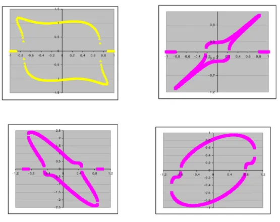
ones. Figure 3 shows four examples, computed with simulated data, of how the
isovariance curve may look like in the “returns x skewness” plane. All the four curves have two directions that provide, locally, the highest skewness (in absolute values) and
one of the first two directions becomes very close to the latter, the curve becomes closer
to an elliptical shape, as in the two bottom pictures. It is also worth noticing that the
direction that gives a highest (lowest) skewness in one quadrant gives a lowest (highest)
one in the diagonally opposed one.
If the portfolio with the highest skewness is the one further to the right – i.e.,
generating points in the first quadrant, we’ll have a well-behaved efficient set. If it is
further to the left - lying, for instance, in the second quadrant, we’ll have a
discontinuous efficient set, or, if one only wants to work with non-negative skewness
and excess return, the surface must be cut.
-1,5 -1 -0,5 0 0, 5 1 1, 5
-1 -0,8 -0,6 -0,4 -0, 2 0 0, 2 0, 4 0,6 0,8 1
- 1,2 - 0,7 - 0,2 0,3 0,8
- 1 - 0,8 - 0,6 - 0,4 - 0,2 0 0,2 0,4 0,6 0,8 1
- 2,5 - 2 - 1,5 - 1 - 0,5 0 0,5 1 1,5 2 2,5
- 1,2 - 0,8 - 0,4 0 0,4 0,8 1,2
- 1 - 0 ,8 - 0 ,6 - 0 ,4 - 0 ,2 0 0 ,2 0 ,4 0 ,6 0 ,8 1
- 1 ,2 - 0 ,8 - 0 ,4 0 0 ,4 0 ,8 1 ,2
Figure 3: Four possible shapes of isovariance curves in the mean x standardised skewness plane. The curves were generated from actual data points, that is why they look
discontinuous. Beyond being all continuous, the sharp horizontal edges suggested in all but
the one below right do not really characterise cuspids, all being (if conveniently zoomed)
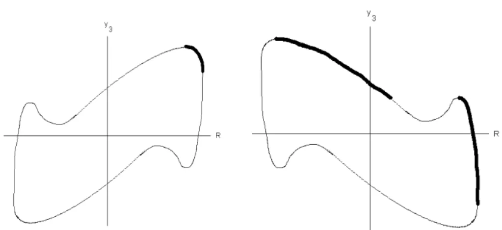
Figure 4 – a qualitative interpretation of several simulations - illustrates two key
cases. The one to the left corresponds to the ideal situation, the part of interest in the
isovariance curves lies in the first quadrant and is a connected set. In the one to the right
– a mirror image of the previous curve -, the global maximum skewness corresponds to
a negative return value. Moreover, the valley of the lowest skewness solution forces a
discontinuity in the optimal set. If the discontinuity is very long, it will imply a great
loss of expected return when jumping from one part to the other of the efficient set,
meaning that we might be better off staying at the right side arch. As a consequence, the
optimal portfolio set may assume many different shapes beyond the well-behaved
paraboloid-like surface in Figure 2(a). In practice, when facing a situation like the one
in the right of Figure 4, the analyst must decide where she wants to pursue the
minimisation algorithm: work in both parts, stay only with the right arch or work with it
and the portion of the other arch in the first quadrant.
Figure 4: Two possible shapes of isovariance curves, with – in bold – the line from the
maximum mean return point to the maximum skewness one. The figure in the left portrays
the ideal situation, in the one in the right, the final efficient surface will have two pieces.
As a final remark on why the isovariance curves may become so complicated, it
should perhaps be reminded that portfolio skewness can become a very complicated
function of R, depending on the (marginal) skewnesses and co-skewnesses between the
different assets. Even with a small number of assets, say three, it is easy to work out a
degree never smaller than three. The “isovariance curves” may then assume different
and complex shapes as illustrated above
5. The efficient frontier
The efficient frontier will be built up by means of the Duality Lemma; in order
to conveniently use it a last proposition is needed:
Proposition 4: Let kR be as in (14) and the kS in (20) be the one related to the highest
skewness line, which is supposed to be unique, THEN kS≥ kR , or, in other words, the angle of the ‘highest skewness line’ is greater than the one of the ‘highest mean (excess)
return line’. Moreover, in the area comprised by these two lines and the positive
(excess) returns half of the mean returns x standardised skewness plane, both Lagrange
multipliers related to programme (1) are positive.
Proof: Let R=1 and consider the (irrestrict) minimum variance (14) which solves the
classical mean-variance problem; there is associated to this pair a standardised skewness
obtained from (15) which is exactly kR. Now take in the ‘highest skewness line’ the
(standardised) skewness corresponding to R=1 , which will be kS. The variance
associated to the constraints 1, kS must be superior to (14) , because this is the (skewness
unconstrained) minimum variance when R=1. But it is also the (mean unconstrained)
minimum variance when skewness equals kS , so the only possibility is that kS ≥ kR . For the second part, we know that λ2 is zero all along the ‘highest mean return
line’ and, from the previous argument, that the ‘highest skewness line’ lies above. Given
that the multipliers are a continuous function of the constraints, let’s examine what
happens with λ2 when we move upwards, in the vertical, from a point on the ‘highest
mean return line’. Along this path, the mean return will be the same but skewness will
be progressively increasing; the fact that departure was from a “Markowitz point” and
the homotethy imply that the minimum variance will also be increasing, so λ2 will
become positive – the optimum is increasing with the restriction - along all lines
progressively passing through the origin at a higher angle than kR. This continues until
one reaches the ‘highest skewness line’ where λ2 is indeed positive whenever the
For λ1 it suffices to repeat the argument now moving horizontally to the right,
from a point on the ‘highest skewness line’ - where, as known, λ1 is zero. The value of
the multiplier when one reaches the other line is, from (2), positive whenever R is.
We are now ready to invoke the duality result. Within the region between the
two canonical lines both multipliers are positive and the Lemma applies to both possible
inversions, namely, maximise skewness, given the same mean and the optimum
variance, or maximise mean excess return given the same skewness and the optimum
variance, so that the efficient frontier is the part of the minimum variance surface
(outlined in the ‘normal case’ in Figure 2(a)) comprised between the vertical planes
passing through the canonical lines. Outside this part, though for a given
mean-skewness pair there exists a minimum variance, as at least one multiplier is negative, it
will be possible to move a little in the optimal surface, along a specified direction,
increasing both members of the pair while simultaneously decreasing the variance; so
that the original pair gives way to an inefficient point.
For computing the optimum, one should then first obtain the canonical lines
described in Proposition 3; vertical – i.e., parallel to the standard deviation axis – planes
through them will circumscribe the efficient set. If a minimum variance portfolio is
sought, provided the k defined by the ratio of the given skewness to the cube of the
given excess return is efficient – i.e., comprised between the two canonical lines the
agent wants to work3 -, the fixed point(s) for the function ϕ below, which is a
re-working of the right-hand side of (11), making 3
3 k
p =
σ and R=1,
) (
)) ( ( ) (
) (
)) ( ( ) (
) ( ) ( )
( 21 3
2 2 4
0
2 3 0 1
2 2 2 4
0
3 2
4 α α
α α
α α
α
α α
α
ϕ ⊗
− − +
− −
= − M−M
A A
A
A k A x
M A
A A
k A A
,
will be the set of weights α . Multiplication of this vector by the given mean excess return will produce the solution.
6. Conclusions
We have shown how to deal, in a general way, with three-moments portfolio
problem, no complete solution to it had been presented till now, in spite of the
nowadays common knowledge that skewness matters. The notation used allowed to
derive compact formulas ready to feed the proper optimisation algorithms. Moreover, a
deep insight on the geometry of the efficient set was obtained, which – beyond its
theoretical interest – is crucial to guide the practical finding of the optimal weights.
The results presented should now be used in several and diversified concrete
situations, to produce a better grasp of when the (simpler) Markowitz solution would lie
too far from the optimum and to improve the knowledge on the different patterns of
multiple local optima. The example carried out in section four, and the complex
structure – in its full generality - of the nonlinear system (7) make these practical
experiments a must. They also seem to announce that the Markowitz solution may be
very inefficient.
Finally, given the need to regularly update optimal portfolios, the framework here
developed must be translated, in a further stage, into a dynamic setting.
Appendix
Proof of the Duality Lemma in section 2:
An extreme value of f(x), at point x*, subject to g−g(x)=0, and h −h(x)=0 must satisfy:
0
2
1 − =
− g h
f D D
D λ λ , at x* . (A.1)
As λ1>0, multiplying (A.1) by -1/λ1, we get: 0
2
1 − =
− f h
g D D
D γ γ , at x* , (A.2) where γ1 =1/λ1 >0 and γ2 =−λ2/λ1 . (A.3)
Given that x* is a minimum of f(x) subject to g−g(x)=0 and h−h(x)=0, the differentiability hypotheses imply that the determinants of the Bordered Hessians
below – where r=3, 4, ..., n , and the symbol ( )rr denotes the square matrix obtained
from the Hessian of the Lagrangian by retaining only the elements of its first r rows and
columns, while ( )r denotes the vector formed with the r first rows of the derivative of
each restriction – exist. Moreover, as strict second-order conditions are assumed, by
Theorem 10.5 in Panik (1976; page 220), they must also be non-negative,
3
ù ê ê ê ë é − − − − − − 0 0 ' ) ( 0 0 ' ) ( ) ( ) ( )
( 1 2
r g r h r g r h rr h g f D D D D H H
H λ λ
. (A.4)
Multiplying the matrix in (A.4) by -1/λ1, we have:
ù
ê ê ê
ë
é − −
0 0 / ' ) ( 0 0 / ' ) ( / ) ( / ) ( ) ( 1 1 1 1 2 1 λ λ λ λ γ γ r g r h r g r h rr h f g D D D D H H H
, where now the sign of each
determinant will be that of (−λ1)r+2 or of (−1)r+2 as λ1>0 . Multiplying the last two rows and columns of each matrix above by λ1:
ú ú ú ù ê ê ê ë
é − −
0 0 ' ) ( 0 0 ' ) ( ) ( ) ( )
( 1 2
r g r h r g r h rr h f g D D D D H H
H γ γ
,
and the determinant signs will not change. Making use of (A.2), these matrices are
identical to: ù ê ê ê ë é + + − − 0 0 ' ) ' ( 0 0 ' ) ( ) ( ) ( ) ( 2 1 2 1 2 1 r h f r h r h f r h rr h f g D D D D D D H H H γ γ γ γ γ γ ;
moreover, their determinants do not change if one subtracts the penultimate row times
2
γ from the last, and does the same for the last two columns:
ù
ê ê ê
ë
é − −
0 0 ' ) ( 0 0 ' ) ( ) ( ) ( ) ( 1 1 2 1 r f r h r f r h rr h f g D D D D H H H γ γ γ γ .
-1/γ1=λ1 > 0 :
ú ú ú ù
ê ê ê
ë é
− −
− −
− −
0 0
' ) (
0 0
' ) (
) ( ) ( )
( 1 2
r f
r h
r f r
h rr
h f
g
D D
D D
H H
H γ γ
. (A.5)
But the matrices in (A.5) are Bordered Hessians, for r=3,...,n , of the problem of
maximising g(x) subject to f − f(x)=0 and h −h(x)=0. Their signs, given the last operation performed, will be those of (−1)r+4 . Equation (A.2) and the fact that (−1)r times the corresponding determinant in (A.5) always gives a positive number (as
0 ) 1 ( ) 1
(− r − r+4 > ) make up a sufficient condition (by the already mentioned Theorem 10.5 in Panik(1976)) for x* to be a strong local maximum of the dual problem.
References
Campbell, J., Lo, A., MacKinlay, C. 1997. The Econometrics of Financial Markets. Princeton University Press, Princeton.
Ingersoll, J. 1975. Multidimensional security pricing. Journal of Financial and Quantitative Analysis 10, 785-798.
Kraus, A., Litzenberger, R. H. 1976. Skewness preference and the valuation of risky assets. Journal of Finance 31, 1085-1100.
Mandelbrot, B. 1963. The variation of certain speculative prices. Journal of Business 36, 394-419.
Panik, M. J. 1976. Classical Optimization: Foundations and Extensions. North-Holland Pub. Co., Amsterdam.