F RADE O CTOBER- 2017

(1)

M

ASTER IN

F

INANCE

M

ASTER

´

S

F

INAL

W

ORK

D

ISSERTATION

P

ERFORMANCE OF

R

ETURN

M

ODELS

:

A

PORTFOLIO

THEORETICAL APPROACH

C

ARLOS

A

UGUSTO

Z

ERPA

F

RADE

(2)

i

M

ASTER IN

F

INANCE

M

ASTER

´

S

F

INAL

W

ORK

D

ISSERTATION

P

ERFORMANCE OF

R

ETURN

M

ODELS

:

A

PORTFOLIO

THEORETICAL APPROACH

C

ARLOS

A

UGUSTO

F

RADE

S

UPERVISION

:

R

AQUEL

M

EDEIROS

G

ASPAR

(3)

ii

A

BSTRACT

(4)

iii

R

ESUMO

O objetivo desta investigação é avaliar o impacto das assunções dos modelos geradores de retornos nas fronteira eficiente e seus portafolios. Isto foi conseguido mediante o trabalho in-sample (assim eliminando o risco de estimação, focando a investigação no risco de modelo) em ambos mercados de ativos financeiros, o Europeo e Americano, nos 7 anos anteriores, considerando ambos, o caso em que shortselling esta permitido como também o caso em que esta proibido. O processo inclui o calculo da fronteira eficiente seguindo as assunções dos modelos geradores de retornos. Em particular o Constant Correlation Model (CCM), o Single-Index Model (SIM) e o modelo de tres factores de Fama e French (1993) Multi-Factor Model (MFM). Para os dois mercados de investimentos, comparamos a fronteira eficiente gerada aplicando MVT nos dados in-sample com a fronteira eficiente dos modelos de retorno seleccionados. Mostramos que o risco do model è importante na aplicação do MVT. Sendo os erros encontrados em todos os modelos consideravel. Também, considerando o risco de modelo para o caso de shortselling proibido, o CCM mostra melhor desempenho que os modelos mais sofisticados. Por outra parte, em condiçoes de shortselling permitido, o SIM mostra melhor desempenho.

K

EYWORDS

(5)

iv

List of Figures

Figure 1- In-Sample MVT Efficient Frontier For Europe………..………. 17

Figure 2 - In-Sample MVT Efficient Frontier For America……… 18

Figure 3 - CCM Efficient Frontier For Europe…...……….19

Figure 4 - CCM Efficient Frontier For America…..………... 21

Figure 5 - SIM Efficient Frontier For Europe...……….. 22

Figure 6 - SIM Efficient Frontier For America………...……… 23

Figure 7 - MFM Efficient Frontier For Europe……...……… 25

Figure 8 - MFM Efficient Frontier For America………...……….. 26

Figure 9- Difference Between [E] And [R] On Europe………...28

Figure 10-Difference Between Mvt And [R] On Europe……… 29

Figure 11-Difference Between [E] And [R] On America………... 30

Figure 12-Difference Between Mvt And [R] On America……….. 31

List of Tables

Table 1 - Composition Of Portfolios For Europe – SSNA……….. 28

Table 2 - Composition Of Portfolios For Europe –SSA……….29

Table 3 - Composition Of Portfolios For America –SSNA………30

Table 4 - Composition Of Portfolios For America –SSA……….. 31

List of Tables in Appendix

Table A. 1 European Investment Opportunity Set……….. 37

Table A. 2 American Investment Opportunity Set……….. 37

Table A. 3 Annualized returns of the European opportunity set for MVT in %... 39

Table A. 4 Correlation Matrix of the European opportunity set for MVT……….. 39

Table A. 5 Annualized returns of the American opportunity set for MVT in %...39

(7)

vi

Table A. 7 Correlation Matrix of the European opportunity set for CCM……….. 41

Table A. 8 Correlation Matrix of the American opportunity set for CCM………. 40

Table A. 9 Annualized expected of the European opportunity set for SIM in %... 41

Table A. 10 Annualized expected of the American opportunity set for SIM in %... 41

Table A. 11 Correlation Matrix of the European opportunity set for SIM……….. 42

Table A. 12 Correlation Matrix of the American opportunity set for SIM………. 43

Table A. 13 Annualized expected of the European opportunity set for MFM in %...42

Table A. 14 Annualized expected of the American opportunity set for MFM in %... 42

Table A. 15 Correlation Matrix of the European opportunity set for MFM…………... 44

Table A. 16 Correlation Matrix of the American opportunity set for MFM…………... 43

List of Abbreviations

MVT: Mean Variance Theory CCM: Constant Correlation Model SIM: Single Index Model

(8)

1

1. Introduction

Popularity of the return models stems primarily from the intuitive appeal of the dichotomy into risk and return. The most well-known two-parameter portfolio models have the following main assumptions: A perfect capital market, investor risk aversion and

two-parameters return distribution implies the important “Efficient set theorem”: The optimal

portfolio for any investor must be efficient in the sense no other portfolio with the same or higher expected return has lower dispersion of return. In the search for the optimal portfolio, Markowitz (1952) developed Mean Variance Theory that has been the basis of the modern portfolio analysis. Introducing the concept of diversification into the investment and security analysis world, the theory was widely accepted and welcomed by those who had the means to use it. MVT bases itself in the assumption that analysts are able to estimate expected returns, future returns reliabilities and correlation across any pair of securities. However, our ability to efficiently estimate MVT inputs is limited. For that reason, there are return generating models that could easily and practically describe and help to forecast correlations. Using such models, we face two type of risk, estimation risk and model risk. The estimation risk comes from the process of obtaining the inputs that each model requires, while the model risk comes from the assumption that each model have on its application. The subject of estimation risk has been widely tested and

studied in recent years even though model risk research it’s not a common topic. The

(9)

2

2. Literature Review

The two-attribute risk and return models are very popular in the economics and finance world for analyzing decisions under uncertainty. Holthausen (1981) denotes that the popularity of the return models stems primarily from the intuitive appeal of the dichotomy into risk and return.

The most well-known two-parameter portfolio model were researched by Tobin (1958) and Markowitz (1959). The main assumptions: A perfect capital market, investor risk aversion and two-parameters return distribution implies the important “Efficient set

theorem”: The optimal portfolio for any investor must be efficient in the sense no other

portfolio with the same or higher expected return has lower dispersion of return.

In the search for the optimal portfolio, its proportions and characteristics, Markowitz (1952, 1959) developed MVT. For over 65 years MVT has been the basis of the modern portfolio analysis. Introducing the concept of diversification into the investment and security analysis world, the theory was widely accepted and welcomed by those who had the means to use it1.

MVT bases itself in the assumption that analysts are able to estimate expected returns, future returns reliabilities and correlation across any pair of securities. However, our ability to efficiently estimate MVT inputs is limited, mostly because of the nature of the correlation structure and the large amount of correlation coefficients to be estimated, see Epps (1981).

Elton and Gruber (1973), Elton, Gruber and Urich (1978), Sharpe (1963) and King (1966), acknowledging the situation and used it as a motivation. Developing return generating models that could easily and practically describe and help to forecast correlations.

(10)

3

When using such models, we face two type of risk, estimation risk and model risk. The estimation risk comes from the process of obtaining the inputs that each model requires, while the model risk comes from the assumption that each model have on its application.

The subject of estimation risk has been widely tested and studied in recent years by Bignozzi and Tsanakas (2015), Cardoso and Gaspar (2016), Jegadeesh, Noh, Pukthuanthong, Roll and Wang (2015) and Siegal and Woodgate (2016) even though

model risk research it’s not a common topic.

The present work focus on the model risk, evidencing the effect that model assumption have in the efficient frontier and relevant portfolios, like minimum variance and tangent portfolio, performing an in-sample analysis of real-life portfolios in the European and American stock market and measuring the biases introduced by well-known return generation models: The Constant Correlation Model (CCM), The Single-Index Model (SIM), and the Fama and French (1993) 3 factors model, as our Multi-Factor Model (MFM).

Section 2.1 deepens into MVT and the computation of the correlation structures. The subsequent sections review the return generating models considered for the analysis. Section 2.2 reviews the Constant Correlation Model, Section 2.3 approach the analysis of the Single Index Model and, finally, Section 2.4 aboard the research developments on the Multi Index Model.

2.1 MVT, Breakthroughs and limitations.

(11)

4

Moreover, MVT served as foundation for several further developments that improved the performance of financial investments through portfolio selection. Among them, we recall MVT as the foundation of equilibrium models, such as CAPM, developed by Lintner (1965), Mossin (1966) and Sharpe (1964).

When applying MVT, there are two important steps. The first is the inputs estimation of the model. The Second, consists in using those inputs to determine the investment opportunity set and the associate efficient frontier. The second part thus, depends strongly on part one.

2.2 Constant Correlation Model

The most common correlation assumption is that past correlation structure hold information about the future average correlation, but do not contain information about individual differences of securities contained in the correlation matrix.

Elton and Gruber (1973) and Elton, Gruber and Urich (1978) tested widely the forecast of future correlations by smoothing the historical correlation matrix data with averaging. They tested both aggregate and disaggregate type of averaging techniques. The Aggregate averaging assumes future pairwise correlation coefficients as the average of all correlation coefficients in the past correlation structure. The disaggregate type of averaging is assumes that an average correlation can be found among a group of securities. Their conclusion is that, even when they found differences in the forecast technique, the differences were small when compared to the forecasting error.

2.3 Single Index Model

(12)

5

whole. The correlation structure across securities is then assumed as the correlation

between the securities’ return and the index. Implicitly, the assumption is that there are

no specific correlations across securities’ returns.

2.4 Multi Factor Model

Multi Factor Models emerged when King (1966) analyzed the impact in co-movement among securities beyond the market’s impact, and found the co-movements within industries.

The efficiency of the MFM in performing accurately forecast directly depends on the definition of the factors used. Elton and Gruber (1973) state that one of the most common approaches in finance is let the data define the factors and to obtain the series of factors that best describes the historical variance-covariance matrix we should analyze past correlation structures. However, they found that even when adding factors to the single-index model resulted in a better description of the historical correlation structure, it also led to a lower prediction accuracy and a decrease in the models performance.

Roll and Ross (1980) found that a MFM needs at least three factors to describe the historical correlation structure. While Dhrymes, Friend and Gultekin (1984) found that, in most cases, more than just three factors are needed and that the exact number depends on the overall number of firms under analysis. Gibbons (1982) found that the number of factors needed is between six and seven.

(13)

6

In terms of the comparison with the SIM, Brennam and Schwartz (1983), Nelson and Schaefer (1983), Elton, Gruber and Naber (1988), and Elton, Gruber and Michaely (1990) refer that MFM tend to be preferable because they might be more relevant. The reasons they suggest the last statement is true is because: The model have an better measure in the impact of changes in the interest rates, reflects the effect introduced by the differences in yield spread among government bonds and singular risk class, reflects the effect introduced by the differences in yield spread among government bonds, corporate bonds, and financial bonds, reflects the effect introduced by the differences in a call’s value and reflects the effect introduced by the differences in tax rates

2.5 Historical comparison between models

It is also important to test how well these models perform using parameters that are estimated based on historical data. At this point, it would be wrong to assume that adding more indexes to the MFM would result in a better performance than the single-index model or the constant correlation model. Having a more complex multi-index model only means that it is possible to reproduce more accurately the historical correlation structure, not that the model will forecast more accurately the future correlation structure.

The constant correlation model was tested extensively with respect to the single-index model, the multi-index model and the very historical correlation structures. In the three previous cases, the use of the constant correlation model, both with aggregate and disaggregate type of averaging, had a better performance. Elton, Gruber and Spitzer (2006) found forecast of future correlation structures with differences that were almost always statistically significant at a 0.05 level. Furthermore, differences in the performance of the portfolio in the four cases were significant enough to have an economic impact. Using the constant correlation model often led to an increase in returns of about 25%.

(14)

7

that suggest that simpler models appears to be better than more complex models, stating the preference as constant correlation model and Sharpe single-index model in that order. Cohen and Pogue (1967) tested the economic significance of the multi-index model (specialized form) against a single-index model. The authors divided the securities in the sample by the standard industrial classification. Both models were run with a market index and an industry index, concluding that the single-index model have more desirable properties since the model is simpler to use and led to lower expected risk than the multi-factor model.

Ledoit and Wolf (2003), observing that the increase in the complexity of the models tends to also increase the random noise that the model picks up, asked them self if combining

models wouldn’t improve the accuracy of the estimations. Deriving rules for combining

results of forecasting from two different techniques, they found that combining the historical correlation structure with the Sharpe single-index model outperforms the individual models. However, in a later study in 2004, the authors found that combining the historical correlation structure with the constant correlation model works even better than their previous study. With the same approach as Ledoit and Wolf, a work performed by Elton, Gruber and Spitzer (2006) researched the use of a two-step procedure to find forecast. The first step is forecasting future average correlation between securities, while the second step is forecasting future difference from the mean. Concluding one, that an exponential smooth or a rolling average of past correlation structure works better in predicting the inputs of the model. And second, that organizing the population into industry groups or characteristics as size and assuming the correlation between securities as the average correlation between each group improves the forecasting results.

(15)

8

3. Data and Methodology

In order to evidence the impact that return generating models assumptions have in the investment opportunity set, the efficient frontier obtained, and the associated portfolios, we propose an in-sample empirical analysis.

Out-of-sample results on the MVT are generally composed of inputs (estimation errors) and model risk resulting from the chosen return generating model (assumptions). In order to mitigate the estimation error and only quantify the effect caused by the return model itself, we have chosen to work in-sample, which means, we worked over realized data. Setting our starting investment period in a past date.

Under this control scenario, we know the “true” in-sample MVT inputs. Since all the returns are realized, we compute the realized expected returns, volatilities and correlations for all securities and built the correlation matrix as the original MVT suggest and consider it the realized scenario.

The reviewing of this section is organized as follows. Section 3.1 presents the data gathered and the methodology used to select it. Section 3.2 focus on the computation of the inputs for the MVT and each of the return generating model considered. Having as a division Subsection 3.2.1 for the Constant Correlation Model, Subsection 3.2.2 for the Single Index Model, Subsection 3.2.3 for the Multi Factor Model inputs. Subsequently, Section 3.3 details the calculation process of the set of portfolios under each method and Section 3.4 the methodology used for the comparison process.

3.1 Data

(16)

9

restrictions in the portfolios, two scenarios are tested for each model considered. The first, short-sell is not allowed (SSNA) and second, short-sell allowed (SSA) for each model.

The components of each investment opportunity set represent the appropriate industries or sectors significantly involved in each market place so that each is a fair representation of the whole market. The number of stocks chosen was set in order to generate well enough diversified portfolios, thus, mitigating in its most efficient way the idiosyncratic risk associated. As Reilly (1985) suggests in his research, considering between 12 to 18 stocks should be enough. Mao (1970) and Sharpe (1972) also researched the optimal diversification of portfolios, reaching the conclusion that, in general, the benefits derived from diversification increase with the number of securities but at a decreasing rate. While the cost of diversification increase with the number of securities at an increasing rate, acknowledging that after the 20th_{stock, the benefit from increasing the diversification} does not compensate the increase in the cost of diversification. The data gathered was the daily securities’ price and the risk free rate both from the 01/01/2010 to the 31/12/2016, a seven year investment period.

Europe’s opportunity set is built of 19 EuroStoxx 50’s stocks, each representing one

Stoxx All Europe 800 super sector. The index selected for the single-index model is the EuroStoxx 502. America’s opportunity set is built of 16 S&P500’s stocks, each representing one Global Industry Classification Standard (GICS) super sector. The index selected for the single-index model is the S&P500 itself. See Table A.1 and A.2 for details on the exact shares considered for the each investment opportunity set.

Common daily stock prices are retrieved from Yahoo Finance. The risk free rates comes from the European Central Bank and the Federal Reserves for Europe and America, respectively. Book to market ratio and market capitalizations used in the Fama and French 3 factors MFM are retrieved from Bloomberg.

2_{Selected because represents the performance of the 50 largest companies among the 19 supersectors in}

(17)

10

3.2 Computation of models inputs

The inputs to generate the efficient frontiers and the set of portfolios which are compared in this work are the securities returns and the correlation structure. Each model specifies the calculation of the inputs under different specification, as stated in the literature review. At this point, it is important to remember that the main goal of this work is to analyze the impact of using return models to obtain MVT inputs.

3.2.1 The true MVT Inputs

We focus our study on the expected returns and correlation matrix resulting from the in-sample data. Creating a vector 𝑅̅𝑀𝑉𝑇composed of the annual return of each of the stocks for each opportunity set and a matrix 𝑉𝑀𝑉𝑇 composed with the correlations between the same returns. The above values are the inputs of the true MVT scenario.

This data serves to achieve the MVT efficient frontier, used as benchmark throughout this study, being compared with the other models efficient frontiers. Having this in consideration, these parameters are referred to as true expected returns and true correlation structure. Anything else referred to as true is assumed to be related with these same parameters or model. 𝑅̅𝑀𝑉𝑇and 𝑉𝑀𝑉𝑇are available in the appendix under Table A.3 and Table A.4, respectively, for the European opportunity set and Table A.5 and Table A.6, respectively, for the American opportunity set.

3.2.2 Constant Correlation Model Inputs

(18)

11

equal due to the fact that the input is the same, the standard deviation) was computed using an aggregate averaging technique, following the below formula, as the replacement of the pairwise correlation between each securities return.

ρ = ∑Ni=1N∗(N−1)∑Nj=1ρij 2

(1)

3.2.3 Single Index Model Inputs

For the Single Index Model (SIM), the inputs were computed following William Sharpe (1963) research. Using the data gathered, an auto-regression model was developed between the return of each securities and the return of the index chosen. With such

auto-regression model, we found the parameters α and β for each security. The before

mentioned parameters represent the independent and dependent, respectively, part on the securities return on the market. The annual mean return 𝑅̅𝑆𝐼𝑀 (available in the appendix under Table A.9 for the European opportunity set and Table A.10 for the American opportunity set) of each security was computed using the following formula:

𝑅𝑖 = 𝛼𝑖+ 𝛽𝑖∗ 𝑅𝑀 (2)

The Correlation Matrix 𝑉𝑆𝐼𝑀(available in the appendix under Table A.11 for the European opportunity set and Table A.12 for the American opportunity set)was computed

according to the model’s specifications, following the below formulas:

𝜎𝑖2 = 𝛽𝑖2∗ 𝜎𝑅𝑀2 (3)

𝜎𝑖𝑗2 = 𝛽𝑖∗ 𝛽𝑗 ∗ 𝜎𝑅𝑀2 (4)

3.2.4 Multi-Factor Model Inputs

For the Multi-Factor Model (MFM), the inputs were computed following Fama and French (1993) research. Using the data gathered, an auto-regression model was developed between the return of each securities and the models parameters. Such parameters include the markets excess return, which is assumed to be the return on the Index chosen minus the risk-free rate, the size premium and the value premium.

(19)

12

asset. This portfolios are: Small size companies with low book to market value of its assets (S/L), Small size companies with medium book to market value of its assets (S/M), Small size companies with high book to market value of its assets (S/H), Big size companies with low book to market value of its assets (B/L), Big size companies with medium book to market value of its assets (B/M) and Big size companies with high book to market value of its assets (B/H).

Once the six portfolios are computed, the Size premium SMB (small minus big) and the HML (high minus low) components required by the model were computed as follows:

𝑆𝑀𝐵 = 1_{3 ∗ (𝑆/𝐿 + 𝑆/𝑀 + 𝑆/𝐻) −}1_{3 ∗ (𝐵/𝐿 + 𝐵/𝑀 + 𝐵/𝐻) (5)}

𝐻𝑀𝐿 =1₂∗ (𝑆/𝐻 + 𝐵/𝐻) −1₂∗ (𝑆/𝐿 + 𝐵/𝐿) (6)

With such auto-regression model, we found the parameters α, β1, β2 and β3 for each security. The annual mean return 𝑅̅𝑀𝐹𝑀 (available in the appendix under Table A.13 for the European opportunity set and Table A.14 for the American opportunity set) of each security was computed using the following formula:

𝑅𝑖𝑡− 𝑅𝑓𝑡 = 𝛼𝑖𝑡+ 𝛽𝑖1∗ (𝑅𝑀𝑡− 𝑅𝑓𝑡) + 𝛽𝑖2∗ 𝑆𝑀𝐵 + 𝛽𝑖3∗ 𝐻𝑀𝐿 (7)

The Correlation Matrix 𝑉𝑀𝐹𝑀(available in the appendix under Table A.15 for the European opportunity set and Table A.16 for the American opportunity set) was

computed according to the model’s specifications, following the below formulas:

𝜎𝑖2 = 𝛽𝑖12∗ 𝜎(𝑅𝑀−𝑅𝑓)2+ 𝛽𝑖22∗ 𝜎(𝑆𝑀𝐵)2+ 𝛽𝑖32∗ 𝜎(𝐻𝑀𝐿)2 (8)

𝜎𝑖𝑗2 = 𝛽𝑖1∗ 𝛽𝑗1∗ 𝜎(𝑅𝑀−𝑅𝑓)2+ 𝛽𝑖2∗ 𝛽𝑗2∗ 𝜎(𝑆𝑀𝐵)2+ 𝛽𝑖3∗ 𝛽𝑗3∗ 𝜎(𝐻𝑀𝐿)2 (9)

3.3 Efficient frontier and set of portfolios computation

Once the inputs of each model were computed accordingly, the method used to obtain the efficient frontier and set of portfolios to analyze (naïve portfolio, minimum variance portfolio and maximum Sharpe ratio portfolio) was the same, indifferently of the model used to compute the inputs. Using the formulas as follows:

𝑅̅𝑝 = 𝑋𝑇∗ 𝑅̅ (10)

(20)

13 Where:

𝑅̅: is the returns matrix

X: is the proportion of each security matrix V: is the correlation matrix between securities

The minimum variance portfolio was obtain such that the variance of the portfolio 𝜎_𝑝was minimum:

𝑀𝑖𝑛𝑥𝑎,𝑥𝑏,𝑥𝑐,…,𝑥𝑛𝜎2𝑝,𝑥 = 𝑥𝑎2𝜎𝑎2+ 𝑥𝑏2𝜎𝑏2+ 𝑥𝑐2𝜎𝑐2 + ⋯ + 𝑥𝑛2𝜎𝑛2+ 2𝑥𝑎𝑥𝑏𝜎𝑎𝑏+

2𝑥𝑎𝑥𝑐𝜎𝑎𝑐+ 2𝑥𝑏𝑥𝑐𝜎𝑏𝑐+ ⋯ + 2𝑥𝑛−1𝑥𝑛𝜎𝑛−1,𝑛 𝑠. 𝑡. 𝑥𝑎+ 𝑥𝑏+ 𝑥𝑐 = 1 (12)

In matrix expression:

𝑀𝑖𝑛𝑥𝜎2𝑝,𝑥 = 𝑥′∑𝑥 𝑠. 𝑡. 𝑥′1 = 1 (13)

The tangent portfolio was obtain such that the Sharpe ratio was maximized.

𝑀𝑎𝑥𝑥𝑅𝑝 = 𝑥′𝑅 𝑠. 𝑡. 𝜎2𝑝 = 𝑥′∑𝑥 = 𝜎2𝑝,0 𝑎𝑛𝑑 𝑥′1 = 1 (14)

To compute the portfolio frontier in (𝑅, 𝜎) space (Markowitz bullet) we only need to find two efficient portfolios. The remaining frontier portfolios can then be expressed as convex combinations of these two portfolios. The following proposition describes the process for the three risky asset case using matrix algebra.

Let 𝑥 = (𝑥_𝑎, 𝑥_𝑏, 𝑥_𝑐)′ and 𝑦 = (𝑦_𝑎, 𝑦_𝑏, 𝑦_𝑐)′ be any two minimum variance portfolios with

different target expected returns 𝑥′𝑅 = 𝑅_𝑝,0 ≠ 𝑦′𝑅 = 𝑅_𝑝,1. That is, portfolio 𝑥 solves

𝑀𝑖𝑛𝑥𝜎2𝑝,𝑥 = 𝑥′∑𝑥 𝑠. 𝑡. 𝑥′𝑅 = 𝑅𝑝,0 𝑎𝑛𝑑 𝑥′1 = 1,

And portfolio 𝑦 solves

𝑀𝑖𝑛𝑦𝜎2𝑝,𝑦 = 𝑦′∑𝑦 𝑠. 𝑡. 𝑦′𝑅 = 𝑅𝑝,1 𝑎𝑛𝑑 𝑦′1 = 1.

(21)

14

𝑧 = 𝛼. 𝑥 + (1 − 𝛼)𝑦 = [𝛼𝑥𝛼𝑥𝑎𝑏+ (1 − 𝛼)𝑦+ (1 − 𝛼)𝑦𝑎𝑏

𝛼𝑥𝑐+ (1 − 𝛼)𝑦𝑐

] (15)

Then the portfolio 𝑧 is a minimum variance portfolio with expected return and variance given by:

𝑅𝑝,𝑧 = 𝑧′𝑅 = 𝛼. 𝑅𝑝,𝑥+ (1 − 𝛼)𝑅𝑝,𝑦, (16)

𝜎2

𝑝,𝑧= 𝑧′∑𝑧 = 𝛼2𝜎2𝑝,𝑥+ (1 − 𝛼)2𝜎2𝑝,𝑦+ 2𝛼(1 − 𝛼)𝜎𝑥𝑦, (17)

Where

𝜎2

𝑝,𝑥 = 𝑥′∑𝑥, 𝜎2𝑝,𝑦 = 𝑦′∑𝑦, 𝜎2𝑥,𝑦= 𝑥′∑𝑦.

3.4 Comparison Process

In order to perform a standardized and rational comparison between models, three methods were selected. The first method includes to compute the difference in risk (volatility) for each level of return for the expected and realized efficient frontiers of each model. The lower this difference is, the closest is the expected from the realized efficient frontier. Second method includes to compute the difference in risk (volatility) for each level of return for the control MVT and realized efficient frontier of each model. The lower this difference is, the closest is the expected from the realized efficient frontier. Lastly, the third method was developed specially for the purpose of measuring the difference between the compositions of portfolios. The difference ratio takes the form of the following formula:

𝐷𝑖𝑓𝑓𝑒𝑟𝑒𝑛𝑐𝑒 𝑟𝑎𝑡𝑖𝑜𝑥,𝑦 = ∑ (𝑥𝑖

𝑦 _{− 𝑥} 𝑖𝑧)2 𝑛

𝑖=1

∑ (𝑥𝑛 _𝑖𝑦 − 𝑥_𝑖𝑛𝑎𝑖𝑣𝑒₎2 𝑖=1

(18)

Where:

n: Is the number of assets

(22)

15

The lower this index is, the closest is the composition of the model’s portfolios from the

control MVT portfolio’s composition compared to the naïve portfolio.

The above mentioned ratio was set up to test the intrinsic fact that, even when two portfolios can be a perfect match when being compared considering the return and volatility, that does not mean they have the same combination of assets and composition.

(23)

16

4. Results

The present chapter aboard the results obtained by applying the methodology explained in the last chapter to the data gathered. It is divided into two main sections, first, Section 4.1 covers the results obtained for the European opportunity set. The same section is subdivided in six subsection, Subsection 4.1.1 for MVT results, 4.1.2 for CCM results, 4.1.3 for SIM results, 4.1.4 for MFM results, 4.1.5 for the overall differences between the results obtained from each model and, finally, Subsection 4.1.6 for the combination results regarding each models relevant portfolios. The second part, Section 4.2 covers the results obtained for the American opportunity set. Also following the same standards as the previous section, it is subdivided into Subsection 4.2.1 for MVT results, 4.2.2 for CCM results, 4.2.3 for SIM results and finally, Subsection 4.2.4 for MFM results, 4.2.5 for the overall differences between the results obtained from each model and, finally, Subsection 4.2.6 for the combination results and comparison regarding each models relevant portfolios.

4.1 True Efficient Frontiers and Optimal Portfolios

In the following section, the results obtained by applying MVT to the European and American opportunity sets are shown. The graphs presents the efficient frontiers with their respective minimum variance and tangent portfolio. Also, it provides the position of the naïve portfolio.

4.1.1 European MVT Efficient Frontier

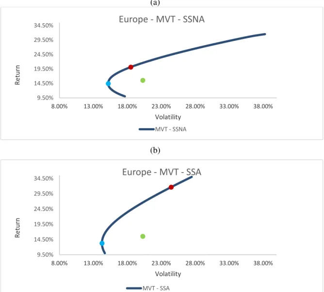
The below Figure 1 (a) presents the efficient frontier obtained by applying the MVT to the European dataset with short-sell not allowed. The tangent portfolio shows a return of 20.13% and a standard deviation of 18.52% while the minimum variance portfolio shows a return of 14.41% and a standard deviation of 15.19%

(24)

17

standard deviation of 24.46% while the minimum variance portfolio shows a return of 13.26% and a standard deviation of 14.27%

Figure 1- In-Sample MVT Efficient Frontier for Europe (a)

(b)

Efficient frontier for the in-sample MVT in the European investment market, both for (a) short-sell

restricted and (b) short-sell allowed

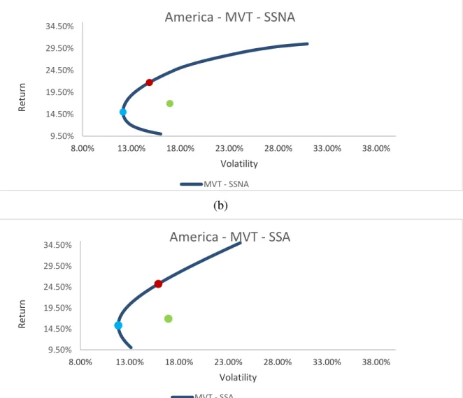
4.1.2 American MVT Efficient Frontier

The below Figure 2 (a) presents the efficient frontier obtained by applying the MVT to the American dataset with short-sell not allowed. The tangent portfolio shows a return of

9.50% 14.50% 19.50% 24.50% 29.50% 34.50%

8.00% 13.00% 18.00% 23.00% 28.00% 33.00% 38.00%

R

et

u

rn

Volatility

Europe - MVT - SSNA

MVT - SSNA

9.50% 14.50% 19.50% 24.50% 29.50% 34.50%

8.00% 13.00% 18.00% 23.00% 28.00% 33.00% 38.00%

R

et

u

rn

Volatility

Europe - MVT - SSA

(25)

18

21.71% and a standard deviation of 14.83% while the minimum variance portfolio shows a return of 14.98% and a standard deviation of 12.13%

Figure 2 (b) presents the efficient frontier obtained by applying the MVT to the American dataset with short-sell allowed. The tangent portfolio shows a return of 25.21% and a standard deviation of 15.91% while the minimum variance portfolio shows a return of 15.30% and a standard deviation of 11.85%

Figure 2 - In-Sample MVT Efficient Frontier for America (a)

(b)

Efficient frontier for the in-sample MVT in the American investment market, both for (a) short-sell

restricted and (b) short-sell allowed

4.2 Using Constant Correlation Model

9.50% 14.50% 19.50% 24.50% 29.50% 34.50%

8.00% 13.00% 18.00% 23.00% 28.00% 33.00% 38.00%

R

et

u

rn

Volatility

America - MVT - SSNA

MVT - SSNA

9.50% 14.50% 19.50% 24.50% 29.50% 34.50%

8.00% 13.00% 18.00% 23.00% 28.00% 33.00% 38.00%

R

et

u

rn

Volatility

America - MVT - SSA

(26)

19

Each subsection presents the graphs of both the expected [E] and realized [R] efficient frontiers with their respective minimum variance and tangent portfolio for each opportunity set. Moreover, each subsection presents the results for both restriction cases, short-sell is allowed and short-sell is not allowed.

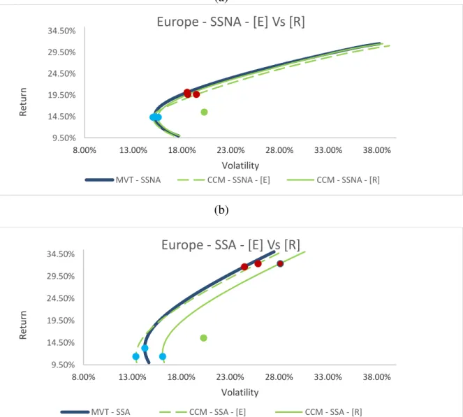
4.2.1 European CCM Efficient Frontier

Figure 3 (a) presents the efficient frontier obtained by applying the CCM to the European dataset with short-sell not allowed. The expected tangent portfolio shows a return of 19.62% and a standard deviation of 19.47% while the expected minimum variance

Figure 3 - CCM Efficient Frontier for Europe (a)

(b)

Efficient frontier for the CCM in the European investment market, both for (a) short-sell restricted and (b)

short-sell allowed. Comparing In-Sample MVT, expected and realized CCM efficient frontier.

9.50% 14.50% 19.50% 24.50% 29.50% 34.50%

8.00% 13.00% 18.00% 23.00% 28.00% 33.00% 38.00%

R

et

u

rn

Volatility

Europe - SSNA - [E] Vs [R]

MVT - SSNA CCM - SSNA - [E] CCM - SSNA - [R]

9.50% 14.50% 19.50% 24.50% 29.50% 34.50%

8.00% 13.00% 18.00% 23.00% 28.00% 33.00% 38.00%

R

et

u

rn

Volatility

Europe - SSA - [E] Vs [R]

(27)

20

shows a return of 14.29% and a standard deviation of 15.02%. The realized tangent portfolio shows a return of 19.62% and a standard deviation of 18.58% while the expected minimum variance portfolio shows a return of 14.29% and a standard deviation of 15.56%.

Figure 3 (b) presents the efficient frontier obtained by applying the CCM to the European dataset with short-sell allowed. The expected tangent portfolio shows a return of 32.36% and a standard deviation of 25.85% while the expected minimum variance portfolio shows a return of 11.40% and a standard deviation of 13.36%. The realized tangent portfolio shows a return of 32.36% and a standard deviation of 28.11% while the expected minimum variance portfolio shows a return of 11.40% and a standard deviation of 16.10%.

4.2.2 American CCM Efficient Frontier

Figure 4 (a) presents the efficient frontier obtained by applying the CCM to the American dataset with short-sell not allowed. The expected tangent portfolio shows a return of 21.93% and a standard deviation of 16.35% while the expected minimum variance portfolio shows a return of 14.06% and a standard deviation of 12.05%. The realized tangent portfolio shows a return of 21.93% and a standard deviation of 15.11% while the expected minimum variance portfolio shows a return of 14.06% and a standard deviation of 12.31%.

(28)

21

Figure 4 - CCM Efficient Frontier for America (a)

(b)

Efficient frontier for the CCM in the America investment market, both for (a) short-sell restricted and (b)

short-sell allowed. Comparing In-Sample MVT, expected and realized CCM efficient frontier.

4.3 Using Single Index Model

9.50% 14.50% 19.50% 24.50% 29.50% 34.50%

8.00% 13.00% 18.00% 23.00% 28.00% 33.00% 38.00%

R

et

u

rn

Volatility

America - SSNA - [E] Vs [R]

MVT - SSNA CCM - SSNA - [E] CCM - SSNA - [R]

9.50% 14.50% 19.50% 24.50% 29.50% 34.50%

8.00% 13.00% 18.00% 23.00% 28.00% 33.00% 38.00%

R

et

u

rn

Volatility

America - SSA - [E] Vs [R]

(29)

22

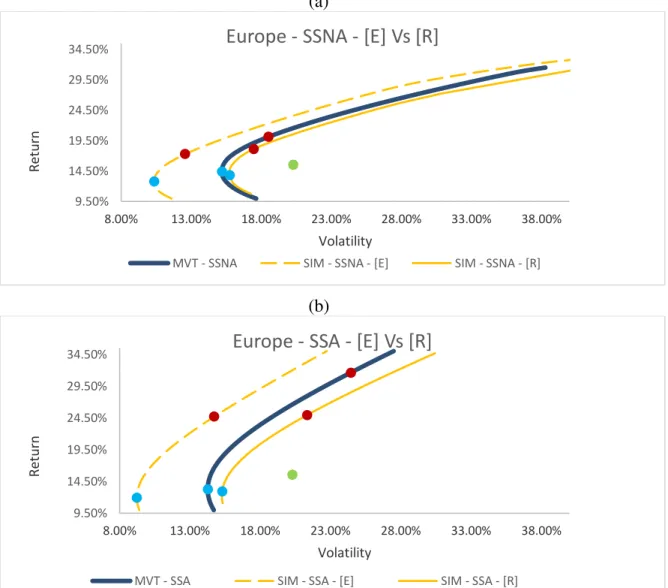
4.3.1 European SIM Efficient Frontier

Figure 5 (a) presents the efficient frontier obtained by applying the SIM to the European dataset with short-sell not allowed. The expected tangent portfolio shows a return of 17.28% and a standard deviation of 12.57% while the expected minimum variance portfolio shows a return of 12.75% and a standard deviation of 10.35%. The realized tangent portfolio shows a return of 18.12% and a standard deviation of 17.46% while the expected minimum variance portfolio shows a return of 13.79% and a standard deviation of 15.75%.

Figure 5 - SIM Efficient Frontier for Europe (a)

(b)

Efficient frontier for the SIM in the European investment market, both for (a) short-sell restricted and (b)

short-sell allowed. Comparing In-Sample MVT, expected and realized SIM efficient frontier.

9.50% 14.50% 19.50% 24.50% 29.50% 34.50%

8.00% 13.00% 18.00% 23.00% 28.00% 33.00% 38.00%

R

et

u

rn

Volatility

Europe - SSNA - [E] Vs [R]

MVT - SSNA SIM - SSNA - [E] SIM - SSNA - [R]

9.50% 14.50% 19.50% 24.50% 29.50% 34.50%

8.00% 13.00% 18.00% 23.00% 28.00% 33.00% 38.00%

R

et

u

rn

Volatility

Europe - SSA - [E] Vs [R]

(30)

23

Figure 5 (b) presents the efficient frontier obtained by applying the SIM to the European dataset with short-sell allowed. The expected tangent portfolio shows a return of

24.70% and a standard deviation of 14.74% while the expected minimum variance portfolio shows a return of 11.96% and a standard deviation of 9.22%. The realized tangent portfolio shows a return of 24.97% and a standard deviation of 21.54% while the expected minimum variance portfolio shows a return of 12.93% and a standard deviation of 15.29%.

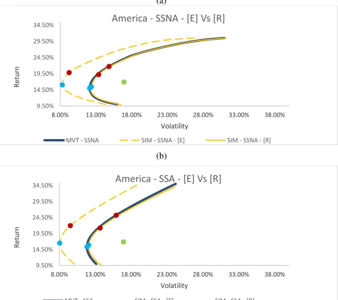
4.3.2 American SIM Efficient Frontier

Figure 6 - SIM Efficient Frontier for America (a)

(b)

Efficient frontier for the SIM in the America investment market, both for (a) short-sell restricted and (b)

short-sell allowed. Comparing In-Sample MVT, expected and realized SIM efficient frontier.

9.50% 14.50% 19.50% 24.50% 29.50% 34.50%

8.00% 13.00% 18.00% 23.00% 28.00% 33.00% 38.00%

R

et

u

rn

Volatility

America - SSNA - [E] Vs [R]

MVT - SSNA SIM - SSNA - [E] SIM - SSNA - [R]

9.50% 14.50% 19.50% 24.50% 29.50% 34.50%

8.00% 13.00% 18.00% 23.00% 28.00% 33.00% 38.00%

R

et

u

rn

Volatility

America - SSA - [E] Vs [R]

(31)

24

Figure 6 (a) presents the efficient frontier obtained by applying the SIM to the American dataset with short-sell not allowed. The expected tangent portfolio shows a return of 19.79% and a standard deviation of 9.26% while the expected minimum variance portfolio shows a return of 16.06% and a standard deviation of 8.30%. The realized tangent portfolio shows a return of 19.21% and a standard deviation of 13.37% while the expected minimum variance portfolio shows a return of 15.49% and a standard deviation of 12.38%.

Figure 6 (b) presents the efficient frontier obtained by applying the SIM to the American dataset with short-sell allowed. The expected tangent portfolio shows a return of 21.93% and a standard deviation of 9.54% while the expected minimum variance portfolio shows a return of 16.48% and a standard deviation of 8.05%. The realized tangent portfolio shows a return of 21.24% and a standard deviation of 13.68% while the expected minimum variance portfolio shows a return of 15.89% and a standard deviation of 12.09%.

4.4 Using Fama

–

French 3 Factors Model

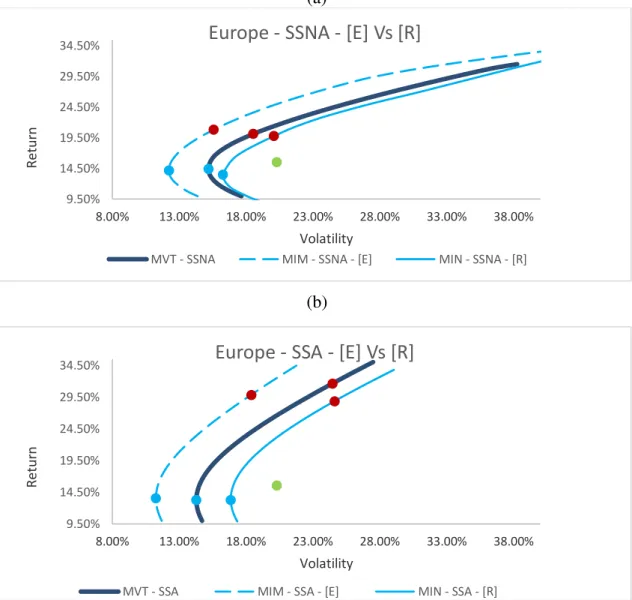
4.4.1 European MFM Efficient Frontier

(32)

25

Figure 7 (b) presents the efficient frontier obtained by applying the SIM to the European dataset with short-sell allowed. The expected tangent portfolio shows a return of 29.85% and a standard deviation of 18.39% while the expected minimum variance portfolio shows a return of 13.55% and a standard deviation of 11.26%. The realized tangent portfolio shows a return of 28.86% and a standard deviation of 24.62% while the expected minimum variance portfolio shows a return of 13.27% and a standard deviation of 16.85%.

Figure 7 - MFM Efficient Frontier for Europe (a)

(b)

Efficient frontier for the MFM in the European investment market, both for (a) short-sell restricted and

(b) short-sell allowed. Comparing In-Sample MVT, expected and realized MFM efficient frontier.

9.50% 14.50% 19.50% 24.50% 29.50% 34.50%

8.00% 13.00% 18.00% 23.00% 28.00% 33.00% 38.00%

R

et

u

rn

Volatility

Europe - SSNA - [E] Vs [R]

MVT - SSNA MIM - SSNA - [E] MIN - SSNA - [R]

9.50% 14.50% 19.50% 24.50% 29.50% 34.50%

8.00% 13.00% 18.00% 23.00% 28.00% 33.00% 38.00%

R

et

u

rn

Volatility

Europe - SSA - [E] Vs [R]

(33)

26

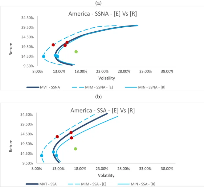
4.2.4American MFM Efficient Frontier

Figure 8 (a) presents the efficient frontier obtained by applying the MFM to the American dataset with short-sell not allowed. The expected tangent portfolio shows a return of 20.43% and a standard deviation of 11.62% while the expected minimum variance portfolio shows a return of 14.40% and a standard deviation of 9.39%. The realized tangent portfolio shows a return of 20.13% and a standard deviation of 14.38% while the expected minimum variance portfolio shows a return of 14.40% and a standard deviation of 12.64%.

Figure 8 - MFM Efficient Frontier for America (a)

(b)

Efficient frontier for the MFM in the America investment market, both for (a) short-sell restricted and (b)

short-sell allowed. Comparing In-Sample MVT, expected and realized MFM efficient frontier.

9.50% 14.50% 19.50% 24.50% 29.50% 34.50%

8.00% 13.00% 18.00% 23.00% 28.00% 33.00% 38.00%

R

et

u

rn

Volatility

America - SSNA - [E] Vs [R]

MVT - SSNA MIM - SSNA - [E] MIN - SSNA - [R]

9.50% 14.50% 19.50% 24.50% 29.50% 34.50%

8.00% 13.00% 18.00% 23.00% 28.00% 33.00% 38.00%

R

et

u

rn

Volatility

America - SSA - [E] Vs [R]

(34)

27

Figure 8 (b) presents the efficient frontier obtained by applying the SIM to the American dataset with short-sell allowed. The expected tangent portfolio shows a return of 23.14% and a standard deviation of 12.74% while the expected minimum variance portfolio shows a return of 13.39% and a standard deviation of 9.16%. The realized tangent portfolio shows a return of 22.53% and a standard deviation of 16.02% while the expected minimum variance portfolio shows a return of 13.48% and a standard deviation of 12.55%.

4.5 Discussion

4.5.2 Efficient frontier comparison for Europe

Figure 9 shows the results obtained by computing the difference in risk (volatility) between expected and realized results in the efficient frontiers for each fixed level of returns, for both SSNA and SSA cases. Figure 10 shows the results obtained by computing the difference in risk (volatility) between MVT and realized results in the efficient frontiers for each fixed level of returns, for both SSNA and SSA cases.

Table 1 and 2 show the composition of both, the minimum variance and the tangent portfolio, for each model used during this research, for both SSNA and SSA cases. At the end of each table, its shown difference in composition ratio. The lower the index is, the closer is the composition of the portfolio to the composition of our control, the MVT.

4.5.2 Efficient frontier comparison for America

Figure 11 shows the results obtained by computing the difference in risk (volatility) between expected and realized results in the efficient frontiers for each fixed level of returns, for both SSNA and SSA cases. Figure 12 shows the results obtained by computing the difference in risk (volatility) between MVT and realized results in the efficient frontiers for each fixed level of returns, for both SSNA and SSA cases.

(35)

28

Figure 9- Difference between [E] and [R] on Europe

Difference in the level of risk (volatility) between expected and realized portfolios for the same level of

returns in the European market.

Table 1 - Composition of Portfolios for Europe – SSNA

Portfolio Composition - Europe - SSNA

Minimum Variance Tangent Portfolio

Securities MVT CCM SIM MIM MVT CCM SIM MIM ABE 1.36% 3.34% 3.98% 0.39% 0.00% 0.00% 0.00% 0.00% AC 0.00% 0.00% 0.00% 1.65% 0.00% 0.00% 0.00% 0.00% AGS 0.00% 0.00% 0.00% 5.33% 0.00% 0.00% 0.00% 2.60% AD 23.56% 21.50% 16.02% 10.06% 11.24% 7.19% 11.54% 0.00% APAM 0.00% 0.00% 0.00% 0.00% 0.00% 0.00% 0.00% 2.51% BAYN 0.00% 0.48% 2.80% 0.11% 0.00% 0.00% 0.00% 0.00% BNP 0.00% 0.00% 0.00% 0.00% 0.00% 0.00% 0.00% 0.00% DTE 0.65% 0.00% 0.46% 0.16% 18.06% 11.67% 9.55% 11.11% EDP 7.14% 3.56% 9.18% 9.79% 0.00% 0.00% 0.00% 0.00% EXO 0.00% 0.00% 0.00% 0.00% 1.87% 12.30% 13.00% 21.03% FCA 0.00% 0.00% 0.00% 0.00% 7.61% 6.46% 1.97% 4.21% GFC 6.23% 4.58% 2.29% 5.27% 5.67% 4.45% 5.13% 10.74% HEIA 16.20% 19.11% 13.01% 8.08% 16.69% 15.18% 6.48% 0.00% NOS 2.73% 0.00% 0.00% 0.00% 0.00% 0.00% 0.00% 0.00% REP 0.00% 0.00% 0.00% 0.00% 0.00% 0.00% 0.00% 0.00% SAP 13.20% 14.81% 4.44% 0.00% 21.37% 27.63% 11.29% 11.01% UCB 12.22% 5.43% 14.98% 10.57% 17.49% 8.65% 15.41% 16.82% UNA 12.71% 27.18% 32.84% 39.80% 0.00% 6.47% 25.64% 19.63% WIE 4.01% 0.00% 0.00% 8.79% 0.00% 0.00% 0.00% 0.35% Difference Ratio 23.0994 38.8913 37.0669 47.7878 47.1580 41.7697

Composition of the minimum variance and tangent portfolios for the European market under the short-sell

restriction. Showing also, the computed Difference Ratio.

0.00% 1.00% 2.00% 3.00% 4.00% 5.00% 6.00% 7.00%

10.00% 15.00% 20.00% 25.00%

ΔV ol at ili ty Returns

Europe - Returns Vs

Δ

Volatilities

(36)

29

Figure 10-Difference between MVT and [R] on Europe

Difference in the level of risk (volatility) between in-sample MVT and realized portfolios for the same level

of returns in the American market.

Table 2-Composition of portfolios for Europe - SSA

Portfolio Composition - Europe - SSA

Securities MVT CCM SIM MIM MVT CCM SIM MIM ABE 8.77% 8.42% 10.27% 7.59% -32.19% -34.10% -20.15% -37.90% AC -3.73% -0.80% 2.61% 3.35% -28.32% -12.51% -1.60% 0.21% AGS -0.88% -4.45% -2.70% 6.45% 7.34% -3.74% -2.29% 11.72% AD 23.11% 24.16% 17.28% 12.75% 22.46% 27.50% 20.30% 15.08% APAM -2.73% -6.60% -5.43% -1.14% 7.78% -1.81% 0.59% 7.08% BAYN -8.14% 5.84% 7.82% 4.00% -16.63% 5.15% 12.96% 1.78% BNP -7.63% -4.99% -10.99% -1.05% -14.68% -12.51% -22.99% -13.71% DTE 1.32% -7.02% 0.95% -0.68% 21.36% 19.90% 9.86% 11.70% EDP 9.70% 8.63% 10.84% 12.63% -10.36% -24.99% -2.55% -4.84% EXO -4.69% -2.81% 0.15% 1.61% 24.75% 24.05% 22.41% 28.08% FCA -2.54% -6.21% -4.64% -3.68% 15.94% 15.84% 8.92% 9.66% GFC 13.07% 9.54% 7.35% 7.12% 26.26% 21.13% 17.59% 21.46% HEIA 15.15% 22.16% 15.42% 10.90% 27.12% 34.89% 17.71% 11.93% NOS 5.64% 1.41% 0.82% -18.34% 4.77% -9.85% 0.31% -13.91% REP 0.55% -1.36% -1.69% -5.96% -27.59% -33.64% -26.49% -38.55% SAP 18.34% 18.45% 9.52% 1.71% 39.23% 46.20% 24.08% 28.38% UCB 13.48% 10.25% 13.25% 12.60% 26.80% 25.48% 16.86% 20.14% UNA 14.63% 29.07% 29.14% 40.48% 6.00% 27.76% 30.02% 34.33% WIE 6.59% -3.69% 0.05% 9.67% -0.04% -14.74% -5.54% 7.36% Difference Ratio 197.0 195.8 4102.9 285.1 2278.5 415.9

Composition of the minimum variance and tangent portfolios for the European market under the short-sell

allowed case. Showing also, the computed Difference Ratio.

0.00% 1.00% 2.00% 3.00% 4.00% 5.00% 6.00% 7.00%

10.00% 15.00% 20.00% 25.00%

Δ V o lat ili ty Returns

Europe - Returns Vs

Δ

Volatilities

(37)

30

Figure 11-Difference between [E] and [R] on America

Difference in the level of risk (volatility) between expected and realized portfolios for the same level of

returns in the American market.

Table 3-Composition of portfolios for America - SSNA

Portfolio Composition - American - SSNA

Securities MVT CCM SIM MIM MVT CCM SIM MIM AMZN 0.51% 0.00% 0.00% 0.00% 15.49% 16.34% 9.20% 14.69% YUM 2.89% 0.00% 6.57% 0.16% 2.69% 3.68% 6.80% 0.00% HSY 15.45% 11.65% 18.88% 15.24% 33.67% 33.31% 23.56% 22.73% CHK 0.00% 0.00% 0.00% 0.53% 0.00% 0.00% 0.00% 0.00% BAC 0.00% 0.00% 0.00% 6.72% 0.00% 0.00% 0.00% 5.43% BLK 0.00% 0.00% 0.00% 0.00% 0.00% 0.00% 0.00% 0.00% ABT 12.31% 12.90% 6.69% 6.76% 0.00% 0.00% 0.00% 0.00% PFE 9.99% 13.13% 10.99% 12.72% 0.00% 0.00% 0.00% 0.00% FDX 0.00% 0.00% 0.00% 0.00% 0.00% 0.00% 0.00% 0.00% GE 0.00% 2.54% 0.00% 0.00% 0.00% 2.01% 0.00% 0.00% AAPL 5.70% 0.00% 1.40% 0.77% 17.90% 18.19% 9.29% 12.82% EA 0.00% 0.00% 1.07% 0.00% 8.22% 6.59% 6.32% 8.02% DOW 0.00% 0.00% 0.00% 0.00% 0.00% 0.00% 0.00% 0.00% AVB 0.00% 1.91% 8.62% 2.59% 0.27% 2.82% 8.32% 3.91% VZ 19.25% 24.71% 16.39% 21.78% 8.74% 12.34% 13.83% 7.76% ED 33.91% 33.16% 29.36% 32.72% 13.03% 4.73% 22.68% 24.65% Difference Ration 108.5195 64.7379 82.8754 513.3331 537.3724 61.0495

Composition of the minimum variance and tangent portfolios for the American market under the short-sell

restriction. Showing also, the computed Difference Ratio.

0.00% 1.00% 2.00% 3.00% 4.00% 5.00% 6.00% 7.00%

10.00% 15.00% 20.00% 25.00%

ΔV

ol

at

ili

ties

Returns

Returns Vs

Δ

Volatilities

(38)

31

Figure 12-Difference between MVT and [R] on America

Difference in the level of risk (volatility) between in-sample MVT and realized portfolios for the same level

of returns in the American market.

Table 4-Composition of portfolios for America – SSA

Portfolio Composition - Europe - SSA

Securities MVT CCM SIM MIM MVT CCM SIM MIM ABE 1.77% -3.94% 1.54% -1.58% 17.90% 17.18% 12.32% 19.33% AC 4.90% 2.14% 8.48% 2.78% 8.93% 8.84% 11.29% -5.57% AGS 15.72% 14.70% 18.35% 15.91% 35.48% 33.61% 23.41% 25.85% AD 0.17% -6.42% -0.56% 1.22% -5.35% -15.49% -3.92% -2.78% APAM -0.52% -5.06% -1.96% 7.83% -7.30% -11.04% -4.14% 10.28% BAYN -9.78% -0.51% -4.33% 1.05% -17.86% -7.33% -8.52% 0.46% BNP 14.74% 15.83% 10.65% 9.87% -14.24% -10.95% -3.33% -15.92% DTE 13.06% 16.27% 14.85% 15.57% 10.68% 7.27% 7.03% 3.74% EDP 1.59% 1.91% -1.31% -3.17% -2.34% -0.52% -1.44% -2.33% EXO 0.92% 6.51% -1.13% -1.71% 4.89% 8.22% -2.08% -6.75% FCA 7.19% 0.13% 3.39% 2.30% 21.39% 19.70% 13.12% 17.09% GFC 0.00% -4.92% 1.91% -3.30% 11.47% 9.26% 7.85% 11.99% HEIA -5.30% -2.91% -5.01% -6.35% 1.10% 0.15% -2.27% -4.09% NOS 2.28% 5.94% 10.12% 5.50% 8.01% 8.77% 12.10% 10.68% REP 21.73% 26.30% 17.21% 21.85% 18.45% 18.57% 16.82% 10.72% SAP 31.53% 34.03% 27.80% 32.24% 8.81% 13.78% 21.75% 27.31% Difference Ration 67.4 28.6 34.9 277.5 228.8 83.4

Composition of the minimum variance and tangent portfolios for the American market under the short-sell

allowed case. Showing also, the computed Difference Ratio.

0.00% 1.00% 2.00% 3.00% 4.00% 5.00% 6.00% 7.00%

10.00% 15.00% 20.00% 25.00%

ΔV

ol

at

ili

ties

Returns

Returns Vs

Δ

Volatilities

(39)

32

5. Conclusion

Based on the methodology applied and the results obtained in the previous section we were able to answer the important question previously set in this research. Which return model performs better and under which circumstances?

To answer the above question, we compared for both opportunity sets, three main results: the difference between the expected and realized efficient frontier and portfolios, the difference between the in-sample MVT (control) and realized efficient frontier and portfolios, and finally, the difference in portfolio composition between in-sample MVT and each model analyzed throughout the present research.

Based on the [E] vs [R] analysis for the SSNA scenario, evidence suggest that, for both opportunity sets, Europe and America, the CCM shows a closer relationship between the expected efficient frontier and the realized one. Followed in order by the MFM and SIM. For the SSA scenario, evidence suggest the same pattern as before, for both opportunity sets, Europe and America, the CCM shows a closer relationship between the expected efficient frontier and the realized one. Followed in order by the MFM and SIM.

Regarding the in-sample MVT vs [R] analysis for the SSNA scenario, evidence suggest that, despite the fact that the chart shows several intersection and not a clear and straight path, the period of the efficient frontier demarked between the minimum variance portfolio and the tangent portfolio for both opportunity sets, Europe and America, the CCM shows a closer relationship between the control efficient frontier and the realized one. Followed in order for Europe by MFM and SIM and for America by SIM and MFM. For the SSA scenario, evidence suggest a divided scenario, for both opportunity sets, Europe and America, before the 20% of return in the graph, the SIM shows a closer relationship between the in-sample MVT efficient frontier and the realized one. Followed in order for Europe by CCM and MFM and for America by MFM and CCM. After the 20% of return, America continuous to show the pattern of SIM first but changing to second CCM and third MFM. While Europe changes to MFM, SIM, and CCM. Being MFM and SIM particular close to each other.

For the composition analysis and judging by the results of the difference ratio for the SSNA scenario, evidence suggests that, for both opportunity sets, Europe and America,

(40)

33

model’s one. Followed in order for Europe by SIM and MFM and for America by MFM

and SIM. For the SSA scenario, evidence suggests that, for both Europe, the CCM shows

a closer relationship between the control portfolio’s composition and the model’s one for

both the minimum variance and tangent portfolio. Followed in order for the minimum variance portfolio by SIM and MFM and for the tangent portfolio by MFM and SIM. For America, the minimum variance portfolio shows a priority of SIM, MFM and CCM while the tangent portfolio shows a priority of CCM, SIM and MFM.

Finally, based on all the evidence stated above, we can conclude that, if we only consider the model risk, for investors seeking a short-sell not allowed scenario, in both the Europe and America opportunity sets, the chosen model should be the simplest one, the CCM. Since it shows closest results to the in-sample MVT (Control) on risk-return basis and also in composition of portfolios. However, to investors seeking a short-sell allowed scenario, in both the Europe and America opportunity sets, the chosen model should be the SIM. Since it shows closest results to the in-sample MVT (Control) on risk-return basis even though CCM shows a closest result in composition of portfolios.

(41)

34

References

Bignozzi, A. Tsanakas, A. (2016). Parameter Uncertainty and Residual Estimation Risk. The Journal of Risk and Insurance, 83 (1), 949–978

Brennan, M.J. Schwartz, E.S. (1985). On the Geometric Mean Index: A Note. Journal of Financial and Quantitative Analysis. XX(1), 119–122.

Burmeister, E. Wall, K. (1986). The Arbitrage Pricing Theory and Macroeconomic Factor Measures. Financial Review. 2, 1–20.

Cardoso, J.M. Gaspar, R. (2016). Robust Mean Variance. Available at ISEG: https://www.iseg.ulisboa.pt/aquila/getFile.do?fileId=643683&method=getFile.

Chan, L.K.C. Karceski, J. Lakonishok, J. (1999). On Portfolio Optimization: Forecasting Covariances and Choosing the Risk Model. Review of Financial Studies. 12, 263–278. Chen, N. Roll, R. Ross, S. (1986). Economic Forces and the Stock Market. Journal of Business. 59, 386–403.

Cohen, K. Pogue, J. (1967). An Empirical Evaluation of Alternative Portfolio Selection Models. Journal of Business. 46, 166–193.

Dhrymes, P.J. Friend, I. Gultekin, N.B. (1984). A Critical Reexamination of the Empirical Evidence on the Arbitrage Pricing Theory. Vol Journal of Finance. 39, Issue 2. 323–346 Elton, E.J. Gruber, M.J. (1973). Estimating the Dependence Structure of Share Prices-Implications for Portfolio Selection. Journal of Finance. vol. 28, issue 5, 1203-32. Elton, E.J. Gruber, M.J. Michaely, R. (1990). The Structure of Spot Rates and Immunization. Journal of Finance. XLV(2), 621–641.

Elton, E. Gruber, M. Naber, P. (1988). Bond Returns, Immunization and the Return Generating Process. in M. Sarnat and G. Szego (eds.), Studies in Banking and Finance, Essays in Memory of Irwin Friend (New York: North-Holland, 1988).

Elton, E.J. Gruber, M.J. Spitzer, J. (2006). Improved Estimates of Correlation Coefficients and Their Impact on the Optimum Portfolios. European Financial Management. 12(3), 303–318.

Elton, E.J. Gruber, M.J. Urich, T. (1978). Are Betas Best?. Journal of Finance. XIII(5), 1375–1384.

(42)

35

Fama, Eugene, and French, Kenneth. (1993). Common Risk Factors in the Returns on Stocks and Bonds. Journal of Financial Economics, 33, 3–56.

Gibbons, M.R. (1982) Multivariate Tests of Financial Models: A New Approach. Journal of Financial Economics. 10, 3–27.

Holthausen, D. (1981). A Risk-Return Model with Risk and Return Measured as Deviations from a Target Return. American Economic Review, 1981, 71 (1), 182-88 Jegadeesh, N. Noh, Joonki. Pukthuanthong, K. Roll, R. Wang, J. (2015). Empirical Tests of Asset Pricing Models with Individual Assets: Resolving the Errors-in-Variables Bias in Risk Premium Estimation. Available at SSRN: https://ssrn.com/abstract=2664332 or http://dx.doi.org/10.2139/ssrn.2664332

King, B. (1966). Market and Industry Factors in Stock Price Behavior. Journal of Business. 39, 139–140.

Ledoit, O. Wolf, M. (2003). Improved Estimation of the Covariance Matrix of Stock Returns with an Application to Portfolio Selection. Journal of Empirical Finance. 10(5), 603–624.

Lintner, J. (1965). The Valuation of Risk Assets and the Selection of Risky Investments in Stock Portfolios and Capital Budgets. Review of Economics and Statistics. XLVII, 13– 37.

McElroy, M.B. (1988). Joint Estimation of Factor Sensitivities and Risk Premia for the Arbitrage Pricing Theory. Journal of Finance, 1988, vol. 43, issue 3, 721-33.

Mao, C.T.J. (1970). Essentials of Portfolio Diversification Strategy. Journal of Finance. V(5), 1109–1121.

Markowitz, H. (1952). Portfolio selection*. The journal of finance, 7(1), 77-91.

Markowitz, H. (1959). Portfolio selection: efficient diversification of investments. Cowies Foundation Monograph, (16).

Mossin, J. (1966). Equilibrium in a Capital Asset Market. Econometrica. 34, 768–783.

Nelson, J. Schaefer, S. (1983). The Dynamics of the Term Structure and Alternative Portfolio Immunization Strategies. in G. Bierwag, G. Kaufman, and A. Toevs (eds.), Innovations in Bond Portfolio Management: Duration Analysis and Immunization (Greenwich, CT: JAI Press, 1983).

(43)

36

Roll, R. Ross, S. (1980) An Empirical Investigation of the Arbitrage Pricing Theory. The Journal of Finance. 35, 1073–1103.

Sharpe, W.F. (1963). A Simplified Model for Portfolio Analysis. Management Science, 1963, vol. 9, issue 2, 277-293

Sharpe, W.F. (1964). Capital Asset Prices: A Theory of Market Equilibrium under Conditions of Risk. The Journal of Finance, Vol. 19, No. 3. 425-442

Sharpe, W.F. (1972). Simple Strategies for Portfolio Diversification: Comment. Journal of Finance, VII(1), 127–129.

Siegal, A. Woodgate, A. (2015). How Much Error Is in the Tracking Error? The Impact of Estimation Risk on Fund Tracking Error. The Journal of Portfolio Management. 41(2), 84-99.

(44)

37

Appendix

Table A. 1 European Investment Opportunity Set

SuperSector Stoxx All Europe 800 Country Name Symbol Industrial Goods & Services ES Abertis Infraestructuras S.A. ABE.MC Travel & Leisure FR Accor SA AC.PA Insurance BE Ageas SA/NV AGS.BR Retail NL Ahold Delhaize AD.AS Basic Resources LU Aperam APAM.AS Chemicals DE Bayer Aktiengesellschaft BAYN.DE

Banks FR BNP Paribas BNP.PA

Telecommunication DE Deutsche Telekom DTE.F

Utility PT EDP EDP.LS

Financial Services IT Exor N.V. EXO.MI Automobile & Parts IT Fiat Chrysler FCA.MI Real State FR Gecina SA GFC.PA Food & Beverage NL Heineken N.V. HEIA.AS

Media PT NOS SGPS NOS.LS

Oil & Gas ES Repsol S.A. REP.MC

Technology DE SAP SE SAP.F

Health Care BE UCB UCB.BR

Personal & Household Goods NL Unilever N.V. UNA.AS Construction & Materials AT Wienerberger AG WIE.VI

Table A. 2 American Investment Opportunity Set

(45)

39

Table A. 3 Annualized expected returns of the European opportunity set for MVT in %

= 7.0 11.7 15.7 14.0 19.0 14.1 12.6 33.7 8.5 23.6 27.2 15.9 15.1 12.0 5.9 17.2 16.4 13.4 11.5

Table A. 4 Correlation Matrix of the European opportunity set for MVT

0.065 0.039 0.051 0.019 0.055 0.034 0.055 0.025 0.031 0.048 0.052 0.028 0.020 0.033 0.046 0.023 0.022 0.021 0.026 0.039 0.103 0.062 0.023 0.074 0.047 0.074 0.032 0.034 0.068 0.078 0.043 0.029 0.040 0.051 0.033 0.028 0.027 0.039 0.051 0.062 0.145 0.022 0.080 0.045 0.098 0.036 0.041 0.072 0.085 0.043 0.023 0.050 0.066 0.033 0.033 0.025 0.038 0.019 0.023 0.022 0.042 0.030 0.024 0.028 0.021 0.018 0.026 0.029 0.017 0.017 0.017 0.023 0.016 0.016 0.020 0.016 0.055 0.074 0.080 0.030 0.212 0.059 0.098 0.042 0.044 0.085 0.098 0.050 0.025 0.049 0.076 0.037 0.030 0.026 0.057 0.034 0.047 0.045 0.024 0.059 0.072 0.059 0.033 0.029 0.053 0.058 0.032 0.027 0.032 0.045 0.032 0.030 0.030 0.031 0.055 0.074 0.098 0.028 0.098 0.059 0.155 0.046 0.049 0.089 0.099 0.050 0.028 0.052 0.080 0.038 0.031 0.032 0.051 0.025 0.032 0.036 0.021 0.042 0.033 0.046 0.243 0.027 0.039 0.039 0.024 0.018 0.025 0.036 0.025 0.017 0.021 0.023 0.031 0.034 0.041 0.018 0.044 0.029 0.049 0.027 0.064 0.039 0.042 0.025 0.017 0.034 0.040 0.021 0.019 0.020 0.022 = 0.048 0.068 0.072 0.026 0.085 0.053 0.089 0.039 0.039 0.121 0.115 0.044 0.028 0.044 0.062 0.037 0.031 0.031 0.043 0.052 0.078 0.085 0.029 0.098 0.058 0.099 0.039 0.042 0.115 0.193 0.047 0.030 0.049 0.071 0.039 0.034 0.032 0.049 0.028 0.043 0.043 0.017 0.050 0.032 0.050 0.024 0.025 0.044 0.047 0.062 0.021 0.028 0.034 0.022 0.019 0.020 0.028 0.020 0.029 0.023 0.017 0.025 0.027 0.028 0.018 0.017 0.028 0.030 0.021 0.044 0.018 0.022 0.020 0.017 0.026 0.016 0.033 0.040 0.050 0.017 0.049 0.032 0.052 0.025 0.034 0.044 0.049 0.028 0.018 0.089 0.040 0.022 0.021 0.019 0.031 0.046 0.051 0.066 0.023 0.076 0.045 0.080 0.036 0.040 0.062 0.071 0.034 0.022 0.040 0.107 0.030 0.024 0.027 0.035 0.023 0.033 0.033 0.016 0.037 0.032 0.038 0.025 0.021 0.037 0.039 0.022 0.020 0.022 0.030 0.048 0.019 0.021 0.020 0.022 0.028 0.033 0.016 0.030 0.030 0.031 0.017 0.019 0.031 0.034 0.019 0.017 0.021 0.024 0.019 0.061 0.019 0.017 0.021 0.027 0.025 0.020 0.026 0.030 0.032 0.021 0.020 0.031 0.032 0.020 0.026 0.019 0.027 0.021 0.019 0.038 0.015 0.026 0.039 0.038 0.016 0.057 0.031 0.051 0.023 0.022 0.043 0.049 0.028 0.016 0.031 0.035 0.020 0.017 0.015 0.132

Table A. 5 Annualized expected returns of the American opportunity set for MVT in %

F RADE O CTOBER- 2017

M

ASTER IN

F

INANCE

M

ASTER

´

S

F

INAL

W

ORK

D

ISSERTATION

P

ERFORMANCE OF

R

ETURN

M

ODELS

:

A

PORTFOLIO

THEORETICAL APPROACH

C

ARLOS

A

UGUSTO

Z

ERPA

F

RADE

M

ASTER IN

F

INANCE

M

ASTER

´

S

F

INAL

W

ORK

D

ISSERTATION

P

ERFORMANCE OF

R

ETURN

M

ODELS

:

A

PORTFOLIO

THEORETICAL APPROACH

C

ARLOS

A

UGUSTO

F

RADE

S

:

R

M

G

A

BSTRACT

R

ESUMO

K

EYWORDS

Table of Contents

List of Figures

List of Tables

List of Tables in Appendix

List of Abbreviations

1.