• Nenhum resultado encontrado

Hindcasting to measure ice sheet model sensitivity to initial states

N/A
N/A
Protected

Academic year: 2017

Share "Hindcasting to measure ice sheet model sensitivity to initial states"

Copied!
11
0
0

Texto

(1)

The Cryosphere, 7, 1083–1093, 2013 www.the-cryosphere.net/7/1083/2013/ doi:10.5194/tc-7-1083-2013

© Author(s) 2013. CC Attribution 3.0 License.

Geoscientiic

Geoscientiic

Geoscientiic

The Cryosphere

Open Access

Hindcasting to measure ice sheet model sensitivity to initial states

A. Aschwanden1,2, G. Aðalgeirsdóttir3, and C. Khroulev1

1Geophysical Institute, University of Alaska Fairbanks, Fairbanks, Alaska, USA

2Arctic Region Supercomputing Center, University of Alaska Fairbanks, Fairbanks, Alaska, USA 3Danish Meteorological Institute, Copenhagen, Denmark

Correspondence to:A. Aschwanden (aaschwanden@alaska.edu)

Received: 12 November 2012 – Published in The Cryosphere Discuss.: 6 December 2012 Revised: 29 May 2013 – Accepted: 30 May 2013 – Published: 10 July 2013

Abstract.Validation is a critical component of model devel-opment, yet notoriously challenging in ice sheet modeling. Here we evaluate how an ice sheet system model responds to a given forcing. We show that hindcasting, i.e. forcing a model with known or closely estimated inputs for past events to see how well the output matches observations, is a vi-able method of assessing model performance. By simulat-ing the recent past of Greenland, and comparsimulat-ing to obser-vations of ice thickness, ice discharge, surface speeds, mass loss and surface elevation changes for validation, we find that the short term model response is strongly influenced by the initial state. We show that the thermal and dynamical states (i.e. the distribution of internal energy and momentum) can be misrepresented despite a good agreement with some ob-servations, stressing the importance of using multiple obser-vations. In particular we identify rates of change of spatially dense observations as preferred validation metrics. Hindcast-ing enables a qualitative assessment of model performance relative to observed rates of change. It thereby reduces the number of admissible initial states more rigorously than vali-dation efforts that do not take advantage of observed rates of change.

1 Introduction

Realistic projections of ice sheet response to a changing cli-mate should be based on physical understanding of the pro-cesses involved, rather than trend extrapolation of histori-cal observations (Arthern and Hindmarsh, 2006). Ice sheet system models are multi-physics models incorporating such physical process understanding. The main sub-systems are ice dynamics, surface and basal processes, and

thermody-namics. Ideally verification and validation should be done for each model sub-system independently. Verification (i.e. the comparison of results from a numerical approximation to exact solutions of the same continuum model equations) is currently only possible for a few sub-systems (e.g. Bueler et al., 2005; Leng et al., 2013) and in a simple coupled system (Bueler et al., 2007). In engineering, validation is commonly defined as the process of comparing model results to a set of observations adequate to falsify a model (Roache, 1998). Such validation is challenging to apply in ice sheet model-ing; nonetheless attempts have been made (Robison et al., 2010; Burton et al., 2012). Direct validation of substantial sub-systems such as basal hydrology, thermodynamics, and ice dynamics is difficult or impossible as most or all obser-vations available for validation are not linked to a single pro-cess, but are the consequence of a complex interplay between sub-systems.

Here we do not seek to isolate, e.g., the model of ice dy-namics, and evaluate it independently; instead we evaluate how thesystemresponds to a given forcing. In other words we ask the question: “how successful is a state-of-the art ice sheet system model (i.e. the combination of physical models, their numerical approximations and implementations, and particular choices of boundary forcing and initial states) in reproducing observations of quantities such as ice thickness, and their temporal changes?” Even if all sub-systems could be verified and validated independently, testing of the system as a whole is indispensable. Consequently, our definition of “validation” differs from the engineering literature.

(2)

performance of an ice sheet system model. First we initial-ize an ice sheet system model. Second the initialinitial-ized model is integrated forward in time for a period where a wealth of data are available for validation. This produces a hind-cast of this time period. Finally, the hindhind-casts are compared to available observations and the performance of the sys-tem model is evaluated. In an ideal case, when using ap-propriate model physics paired with realistic initial states and boundary conditions, a hindcast and observations should agree to within error bars associated with observations. Such an agreement with all available observations may not occur due to several reasons. Disagreement may arise from uncer-tainties in boundary conditions, unrealistic initial states, in-complete model physics, and inadequate choices in numeri-cal methods, to name a few. Using multiple data sets can help to pin down the source of disagreement. As models evolve, the level of disagreement between observations and model simulation is expected to decrease.

Similar to short-term weather forecasts, a realistic initial state is essential for accurate simulations of the future evo-lution of an ice sheet (Arthern and Gudmundsson, 2010). In this study we use hindcasting to assess an ice sheet sys-tem model’s sensitivity to its initial state. We show that it is possible to get good agreement with observations when too few data sets are used. One may wrongly put too much con-fidence in a given model simulation, not realizing that im-portant properties are misrepresented. In particular, previous studies have often used ice volume (e.g. Stone et al., 2010; Rogozhina et al., 2011; Applegate et al., 2012) for validation of the initial state. Spatially dense observations, especially rates of change, are, however, better metrics to evaluate the quality of initial states (Vaughan and Arthern, 2007). As an example, we show that good agreement between observed and simulated total mass loss can be achieved, and only by comparing observed vs. simulated ice discharge is it possible to identify that the apparent good agreement of the former is due to the wrong reason.

Our manuscript is intended to serve as a guidance for fu-ture studies developing better practices in ice sheet system model validation. We do not identify a preferred initializa-tion procedure. Hindcasting is not limited to our particular choices of an ice sheet model, boundary conditions, and ini-tial states; but is transferable to combinations of these. How-ever, conclusions regarding the performance of initialization procedures may not be transferable. Hindcasting may also be helpful to study other aspects of the ice sheet system model’s behavior. It is, for example, important to assess the sensitiv-ity to climate forcing; but this is not within the scope of our study.

2 Methods

Our choice of ice sheet system model comprises the Paral-lel Ice Sheet Model (PISM; Khroulev and the PISM

Au-thors, 2012) unidirectionally coupled to the high-resolution regional climate model HIRHAM5 (Christensen et al., 2006). HIRHAM5 provides climatic mass balance (sum of the sur-face and internal mass balances, Cogley et al., 2011) and 2 m air temperature for the period 1989–2011 (ERA-interim; Dee et al., 2011). HIRHAM5 performs well over Greenland (e.g. Rae et al., 2012) but formal error estimates are not available. Additional information on PISM and HIRHAM5 is given in the Supplement.

We obtain three initial states by using distinct approaches to modeling the 1989 state of the Greenland ice sheet, in each case based on forward modeling and assumptions about past climate. We choose three initialization methods that have been used in the published literature (e.g. Rogozhina et al., 2011; Greve et al., 2011; Price et al., 2011). Below we de-scribe how we obtain the three initial states.

The first initial state, “constant-climate”, is obtained by running the model for 125 ka using mean values for 1989–2011 of 2 m air temperature and climatic mass bal-ance from HIRHAM5. The 2 m air temperature serves as the boundary condition for the conservation of energy equation, and a lapse rate of 7.1◦C km−1 (Steffen and Box, 2001) is

used to correct for differences between the fixed surface el-evation that HIRHAM5 uses and the time evolving modeled elevation. No lapse rate correction is applied to the climatic mass balance. “Constant-climate” is expected to be in equi-librium with modeled present-day climate.

The second initial state, “paleo-climate”, closely follows the SeaRISE initialization procedures (Bindschadler et al., 2013). To obtain this initial state we make the following mod-eling choices. First, we use a positive degree-day scheme to compute the climatic mass balance from surface temperature (Fausto et al., 2009) and model-constrained precipitation (Et-tema et al., 2009). The degree-day factors are the same as in Huybrechts (1998). Second, we account for paleo-climatic variations by applying a scalar anomaly term derived from the GRIP ice core oxygen isotope record (Dansgaard et al., 1993) to the temperature field (Huybrechts, 2002). Then we adjust mean annual precipitation in proportion to the mean annual air temperature change (Huybrechts, 2002). Finally, sea level forcing, which determines the land area available for glaciation, is derived from the SPECMAP marineδ18O

record (Imbrie et al., 1984).

(3)

Our modeling goals are to produce physically consistent initial states of the Greenland ice sheet in 1989 that mimic the overall dynamic state of the whole ice sheet. One can-not achieve agreement with all available observations except through introduction of many tunable parameters, which we do not do.

Also not all observed processes can be adequately repre-sented in the model. For example, increased ice discharge since the late 1990s has been observed (Joughin et al., 2004; Howat et al., 2007) and attributed to an increase in ocean temperatures (Holland et al., 2008; Murray et al., 2010). Un-fortunately, theoretical models to predict such behavior are currently not available (Holland et al., 2008). Therefore no forcing at the ocean boundary is applied.

Properties at the ice sheet bed cannot be directly observed. Ice sheet models may achieve a close fit to observed surface speeds by using data assimilation techniques that invert for a field of basal parameters, for example adjusting the value of the basal traction at each grid location (Morlighem et al., 2010; Price et al., 2011; Gillet-Chaulet et al., 2012). How-ever, the resulting parameter fields may not be applicable for prognostic simulations, as these parameters evolve with time. Moreover, validation cannot rely on observations used in the data assimilation process (van der Veen, 1999).

In this work we adjust only three spatially uniform scalar parameters (Supplement), controlling ice dynamics and basal processes, to achieve a good match with observed surface speeds. Thus observed surface speeds are not a part of the ini-tialization procedure and can be used to validate the model.

At the hindcast stage, all initial states are integrated for-ward in time from 1989 to 2011 using monthly fields of cli-matic mass balance and 2 m air temperature computed by HIRHAM5. Note that identical parameter choices are used to produce all initial states, as well as in the 1989–2011 in-tegration, allowing the influence of initialization procedures to be isolated. All hindcasts are carried out on a grid with horizontal resolution of 2 km.

The hindcasts are then compared to observations listed be-low. Our study does not use all available observations, but the ones used allow drawing robust conclusions about hindcast-ing as a method of assesshindcast-ing model performance. Additional observations that could be used are mentioned in Sect. 4.

Ice thickness and ice volume (Bamber et al., 2013). Er-ror estimates in bed elevation range from a minimum of

±6 m to about±200 m, as a function of distance from an observation and local topographic variability. Surface speeds derived from synthetic aperture radar

(SAR) data from RADARSAT representing an average of the velocity maps for the period 2006–2009. The mean measurement and processing errors are less than 2 m a−1 in areas with low surface slope and additional

slope-dependent error of 3 % in steeper areas (Joughin et al., 2010).

Time series of mass changes from the Gravity Recov-ery and Climate Experiment (GRACE) for the Green-land Ice Sheet, derived from the 10-day 1◦×1◦NASA GSFC mascon solutions for the period January 2004 to December 2010 (Luthcke et al., 2013). Using a linear least-squares fit a mass loss trend of−223 Gt a−1with an uncertainty of±14.3 Gt a−1is obtained.

Surface elevation change measurements from NASA’s Ice, Cloud and land Elevation Satellite (ICESat) for the period October 2003 until November 2009 (Sørensen et al., 2011; Sasgen et al., 2012). Typical uncertainty estimates in ICESat-derived elevation changes are ap-proximately 0.1 m a−1(Howat et al., 2008).

3 Results

3.1 1989 initial state

Figure 1 shows the simulated surface speeds of the three tialized states together with the SAR-derived speeds. All ini-tial states show well-defined ice divides and fast flowing out-let glaciers, with largest differences between simulated and observed speeds occurring in outlet glaciers. The root mean square error (RMSE) of the surface speeds is 43–46 m a−1

(Table 1), having a similar magnitude as obtained in a data assimilation study (38 m a−1, Price et al., 2011).

Compared to observed ice sheet volume (2.93×10⁶km3), numbers for two initialized states are larger, 3.18×10⁶km3 (+9 %) and 3.38×10⁶km3 (+16 %) for “constant-climate” and “paleo-climate”, respectively (Table 1). For “flux-corrected”, simulated ice volume is 2.96×10⁶km3(+1 %). However, observed ice thicknesses are used for initialization and are not available for validation.

Relative differences in ice thickness and surface speeds are shown in Figs. 2 and 3, respectively; absolute differences are shown in the Supplement.

Two initializations, “constant-climate” and “paleo-climate”, overestimate ice thickness near the margin, but underestimate ice thickness in the interior of the ice sheet and in northwest Greenland (Fig. 2). The flux-correction method used to obtain the “flux-corrected” initial state significantly reduces the mismatch between observed and simulated ice thickness except in coastal areas in southeast Greenland.

All three initializations underestimate surface speeds in most major outlet glaciers (Fig. 3).

3.2 Hindcasts

(4)

Fig. 1.Measured and modeled horizontal surface speeds.(a)SAR (Joughin et al., 2010).(b)“constant-climate” hindcast.(c)“paleo-climate” hindcast.(d)“flux-corrected” paleo-climate hindcast. Values are in meters per year. Surface speeds are masked where observed ice thickness is less than 100 m.

Table 1.Initial states and model performance statistics. The RMSE is given for the comparison of simulated surface speeds of the initial state (1989) and the observed 2006–2009 average (Joughin et al., 2010); see Supplement Table 4.1 for details. Also listed are observed ice volume and GRACE trend (Luthcke et al., 2013), the correlation coefficient,r, and the detrended correlation coefficient,. Ice volume is calculated

by integrating ice thickness in space and multiplying by the density of ice (910 kg m−3).

observed “constant-climate” “paleo-climate” “flux-corrected”

ice volume

initial volume [106km3] 2.93 3.17 3.38 2.96 (*) ice thickness

avg difference [m] 99 122 60∗

rms difference [m] 199 244 19∗

surface speed

RMSE [m a−1] 43 46 45

mass trend

trend [Gt a−1] −223 −139 −299 −198

r[-] 0.92 0.99 0.99

˜

r[-] 0.86 0.86 0.83

RMSE [Gt] 130 104 62

Ice thickness was used in the initialization, hence this metric is not available for validation, and only shown for comparison.

coefficient,r, is greater than 0.92 in all experiments,

indicat-ing that both the amplitude and the phase of the mass change signal are well reproduced by the model. The detrended cor-relation coefficients,r˜, are 0.86 (“constant-climate”,

“paleo-climate”) and 0.83 (“flux-corrected”); these are a measure of how well the seasonality is reproduced. Simulated mass loss trends are −139 Gt a−1 for the hindcast based on the “constant-climate” initial state (subsequently shortened to “constant-climate” hindcast), −299 Gt a−1 for the “paleo-climate” hindcast, and−198 Gt a−1for the “flux-corrected” hindcast, differing by a factor of more than 2. Mass loss trends are consistent with respect to the grid resolution (Supplement Table 1) for horizontal grid spacings≤10 km (Supplement Fig. 2). Modeled mean ice discharge is−511,

−581, and−168 Gt a−1 for the “constant-climate”,

“paleo-climate” and “flux-corrected” hindcasts, respectively, over the period 1989–2011. None of the ice discharge time

se-ries shows a significant trend. The modeled mass loss trend is thus due to the evolving climatic mass balance (Fig. 5).

(5)

Fig. 2.Relative difference in ice thickness (model-observation)/observation.(a)“constant-climate” hindcast.(b)“paleo-climate” hindcast.

(c)“flux-corrected” paleo-climate hindcast (only shown for comparison, as ice thickness was part of the initialization). Blue and red colors indicate the model under- and overestimates ice thickness, respectively. Brown color indicates areas where observed ice thickness is zero but the model simulates an ice thickness in excess of 100 m.

Fig. 3.Relative difference in surface speeds (model-observation)/observation.(a)“constant-climate” hindcast.(b)“paleo-climate” hindcast.

(c)“flux-corrected” hindcast. Blue and red colors indicate the model under- and overestimates surface speed, respectively. Areas of observed surface speeds smaller than 100 m a−1(92 % of observed speeds) are masked out because small absolute speed differences result in large relative speed differences. Also uncertainties in SAR-derived surface speeds are higher in slow-flowing areas.

4 Discussion

The discussion is split into two parts. First we discuss the ini-tial states and hindcasts relative to observations. Second we address the suitability of hindcasting as a method to evaluate the performance of an ice sheet system model.

4.1 Initial states and hindcasts

Despite having comparable ice volumes, the three initial states respond differently to the applied climate forcing, and the difference is significant. Therefore reproducing observed ice volume is not a sufficient metric for evaluating initial states.

Surface speeds of most major outlet glaciers are underesti-mated by all three initial states relative to the 2006–2009 av-erage. First, simulated surface speeds of initial states should be compared to the observations from 1989, but observations

(6)

100 m a−1, our parameter choice favors slow flowing ice. RMSE ranges from 43 to 48 m a−1when computed for six different combinations of year of simulation and observation (Supplement Table 4.2). This indicates that the RMSE is not strongly affected by the choice of the combination of year of observation and year of simulation.

The simulations using a “constant-climate” and a “paleo-climate” initialization underestimate and overestimate the mass loss trend, respectively, whereas the “flux-corrected” initialization shows a very good match with observations (i.e. within twice the uncertainty of the GRACE mass loss trend). As mentioned earlier, observations show a rapid increase in ice discharge since the late 1990s, which was attributed to changes at the ocean boundary. Our model does not include ocean forcing that could lead to an increase in simulated ice discharge. Therefore, underestimation of the simulated mass loss trend is expected.

Compared to an observed cumulative mass change of

−1695 Gt for the 2004–2010 period, simulated values are

−1005 Gt (“constant-climate”),−2134 Gt (“paleo-climate”), and −1358 Gt (“flux-corrected”). van den Broeke et al. (2009) report an equal split between surface processes and ice dynamics for 2000–2008 mass loss. By assuming the same equal split between surface processes and ice dy-namics during the 2004–2010 analysis period, we expect a simulated cumulative mass change of ∼ −848 Gt from changes in climatic mass balance, corresponding to a trend of ∼ −113 Gt a−1. Of the three hindcasts only “constant-climate” agrees reasonably well with this estimate.

Because we do not attempt to simulate the observed in-crease in ice discharge, we compare our results to an esti-mate of 1996, representative of the time before the rapid in-crease. For the “constant-climate” and “paleo-climate” ini-tializations, the simulated ice discharge compares well with an estimate of −480 Gt a−1 (van den Broeke et al., 2009, Fig. S3). However, the good agreement is a consequence of consistently overestimating ice thickness (Fig. 2) and under-estimating surface speeds (Fig. 3). The “flux-corrected” ini-tialization underestimates the ice discharge as a result of un-derestimating flow speeds in fast-flowing outlet glaciers. We find that simulated ice discharge is most sensitive to errors in ice thickness, which is in line with Larour et al. (2012b).

Surface elevation changes at Jakobshavn Isbræ, Helheim, and Kangerdlugssuaq are mostly attributed to changes in ma-rine outlet dynamics (Howat et al., 2011) and are therefore not reproduced by our model. The “constant-climate” initial-ization is expected to be in equilibrium with its climate, and, consequently, surface elevation changes should result from the climate forcing, either directly through the applied cli-matic mass balance or, indirectly, through dynamical adjust-ment due to changes in climatic mass balance.

For the “constant-climate” and “paleo-climate” initial-ization, forcing is applied directly, whereas anomalies are used for the “flux-corrected” initialization. For the “paleo-climate” initialization this may result in a shock at the

begin-Table 2.Simulated mass loss trends before and after drift removal for the three hindcasts.

before drift after drift change

correction correction

[Gt a−1] [Gt a−1] [Gt a−1] [%]

“constant-climate” −139 −132 +7 +5

“paleo-climate” −299 −258 +40 +13

“flux-corrected” −198 −169 +30 +15

ning of the hindcast. To study this effect we perform a fourth hindcast where the ERA-interim forcing is applied as anoma-lies relative to the climate forcing at the end of the “paleo-climate” initialization. Results reveal a mass loss trend of

−410 Gt a−1, greater than when the ERA-interim forcing is applied directly, with a surface elevation change pattern very similar to the “flux-corrected” hindcast (not shown).

Generally speaking, a model initialization may generate transients, both wanted (e.g. ongoing adjustments due to forcing history) and unwanted (e.g. from grid refinement), leading to a model drift (Gupta et al., 2012). Even sufficiently long “constant-climate” initializations are not expected to be free of transients; for example, basal hydrology may prevent a steady-state configuration in the mathematical sense (e.g. Kamb et al., 1985). An approach to mitigate the effect of model drift involves calculating model drift and subtracting it from the experiment, implicitly assuming that legacy be-havior does not feed back on the experiment (Bindschadler et al., 2013).

We calculate model drift by performing a reference run for each initial state where the mean climate of the last 10 yr of the initialization is applied. For the GRACE epoch, cumulative mass changes of −50 Gt (“constant-climate”),

−281 Gt (“paleo-climate”), and−205 Gt (“flux-corrected”) are attributed to model drift, corresponding to 5, 13, and 15 % of the total mass change, respectively. After subtracting model drift, simulated mass loss trends are−132 Gt a−1for

the “constant-climate” hindcast,−258 Gt a−1for the

“paleo-climate” hindcast, and−169 Gt a−1for the “flux-corrected”

hindcast (Table 2).

(7)

2005

2006

2007

2008

2009

2010

year

2000

1500

1000

500

0

cumulative mass change [Gt]

GRACE NASA GSFC mascon, 225 Gt a

constant climate, 139 Gt a

paleo climate, 299 Gt a

flux corrected, 198 Gt a

6

5

4

3

2

1

0

cumulative mass change [mm SLE]

Fig. 4.Observed and modeled cumulative mass changes. 10-day solutions from GRACE observations (Luthcke et al., 2013) and simulated daily values starting from the three initial states. The inset figure shows the regression analysis; trends are given in the legend and correlation coefficients are listed in Table 1.

1991199319951997199920012003200520072009

year

500

0

500

1000

ma

ss

flu

x [

Gt

a

]

constant-climate

paleo-climate

flux-corrected

Fig. 5.Simulated mass fluxes from 1990 to 2010. Climatic mass balance (solid line) and ice discharge (dashed line). For comparison the ice discharge estimate for 1996 (van den Broeke et al., 2009) is shown (black dotted line). Time series are smoothed with a 13-month running-average filter.

Model drift is removed by subtracting the surface eleva-tion change time series of the drift experiment from the hind-cast. Drift-corrected surface elevation changes are shown in Fig. 7. The surface elevation changes pattern changes little, still exhibiting large transients not present in observations. There is thus a question of how drift-correction affects the system’s response. This effect remains unquantified and thus quantitative studies are highly desirable.

4.2 Hindcasting as a method of assessing an ice sheet system model

A comparison of observed and simulated rates of change re-quires a reference period covering both observations and sim-ulations. Hindcasting provides simulated rates of change for this reference period. In other words, it adds a temporal di-mension to validation efforts. Hindcasting enables a quali-tative assessment of model performance relative to observed rates of change. This reduces the number of admissible initial states more rigorously than validation efforts that do not take advantage of observed rates of change. As an example, hind-casting allowed us to realize that our flux-correction method produces unrealistic surface elevation changes between 2003 and 2009.

(8)

55°W 45°W 35°W

60°N

65°N

70°N

75°N

80°N a)a)a)a)

55°W 45°W 35°W

b)b)b)b)

55°W 45°W 35°W

c)c)c)c)

55°W 45°W 35°W

d)d)d)d)

2.5

2.0

1.5

1.0

0.5

0.0

0.5

1.0

1.5

2.0

2.5

m

Fig. 6. Observed and modeled surface elevation change from October 2003 to November 2009. (a)ICESat (Sørensen et al., 2011).

(b)“constant-climate” hindcast.(c)“paleo-climate” hindcast.(d)“flux-corrected” paleo-climate hindcast. Values are in meters.

55°W 45°W 35°W

60°N

65°N

70°N

75°N

80°N a)a)a)a)

55°W 45°W 35°W

b)b)b)b)

55°W 45°W 35°W

c)c)c)c)

55°W 45°W 35°W

d)d)d)d)

2.5

2.0

1.5

1.0

0.5

0.0

0.5

1.0

1.5

2.0

2.5

m

Fig. 7.Observed and modeled surface elevation change from October 2003 to November 2009 after subtracting the corresponding reference simulations.(a)ICESat (Sørensen et al., 2011).(b)“constant-climate” hindcast.(c)“paleo-climate” hindcast.(d)“flux-corrected” hindcast. Values are in meters.

records. In consequence of those limitations, a quantitative assessment of model performance is currently not possible with hindcasting.

We have not used all available observations. Additional observations that can be used for validation are, for example, spatially distributed mass loss estimates from GRACE (e.g. Luthcke et al., 2013) and temporal variation in ice surface velocity (Joughin et al., 2010; Moon et al., 2012). The afore-mentioned modeled age field could be compared to dated isochrones. Such a comparison provides a strong validation metric because the age field is, first, representative of long energy timescales and, second, a three-dimensional field (in contrast to, for example, surface elevation). For those reasons an accidental agreement between simulated and observed age of the ice is quite unlikely. Fortunately the number of both remotely sensed and in situ observations is constantly grow-ing. Future studies should take advantage of these data sets for validation.

5 Conclusions

It has become clear that an initial state achieving a good fit with both spatially dense surface speeds and rates of change of total ice mass may still misrepresent important character-istics (ice discharge and ice thickness are two examples). In-formally speaking, it is possible to “get the right result for the wrong reason”. Our analysis identifies spatially dense time series of observations as preferred validation metrics, thus corroborating the assertion of Vaughan and Arthern (2007).

(9)

We have demonstrated that ice sheet system models are capable of transforming climate forcing into simulated mass loss from the ice sheet in a realistic way. Our model suc-cessfully reproduces the seasonal signal and decadal trends in mass loss as well as the velocity structure using only a few ice-sheet-wide parameters. “constant-climate” and “paleo-climate” show reasonable agreement with the observed ice discharge of 1996. However, the subsequent increase is not captured because of missing model physics at the ocean boundary. Clearly, future work should focus on theoretical models of ice–ocean interaction, and their numerical imple-mentations.

The comparison of initialization strategies shows that the model response to climate forcing is sensitive to the initial state on decadal timescales, emphasizing the importance of well-validated initial states for reliable projections. We rec-ommend thorough validation of initial states used for prog-nostic simulations, and hindcasting offers a viable validation strategy. Hindcasting is not limited to our particular choice of an ice sheet system model.

While a direct validation in the engineering sense may not be applicable, our view of ice sheet models as ice sheet sys-tem models allows validation of another type. Furthermore, hindcasting can be part of a concerted effort to validate ice sheet models. Other parts include formal sensitivity analyses to assess error propagation in forward models as, for exam-ple, carried out by Larour et al. (2012a,b). Ultimately, valida-tion may be integrated in statistical frameworks to quantify uncertainties in ice sheet evolution due to different sources of model and observation uncertainty (c.f. Steinschneider et al., 2012, for an example in hydrologic modeling).

Supplementary material related to this article is available online at: http://www.the-cryosphere.net/7/ 1083/2013/tc-7-1083-2013-supplement.pdf.

Acknowledgements. Thanks to A. Arendt, T. Bartholomaus, E. Bueler, M. Fahnestock, W. D. Harrison, R. Hock, D. Po-drasky, and M. Truffer for stimulating discussions. S. B. Luthcke and I. Joughin provided GRACE and SAR data, respectively. J. A. Griggs provided basal topography and ice thickness. L. S. Sandberg Sørensen provided ICESat data, and R. Mottram and F. Boberg provided HIRHAM5 forcing. M. Fahnestock provided the MODIS mosaic. This work was supported by NASA grant No. NNX09AJ38G, by a grant of HPC resources from the Arctic Region Supercomputing Center as part of the Department of Defense High Performance Computing Modernization Program, and by funding from the Ice2Sea programme from the European Union 7th Framework Programme, grant number 226375. Ice2sea contribution number ice2sea077.

Edited by: E. Larour

References

Applegate, P. J., Kirchner, N., Stone, E. J., Keller, K., and Greve, R.: An assessment of key model parametric uncertainties in projec-tions of Greenland Ice Sheet behavior, The Cryosphere, 6, 589– 606, doi:10.5194/tc-6-589-2012, 2012.

Arthern, R. J. and Gudmundsson, G. H.: Initialization of ice-sheet forecasts viewed as an inverse Robin problem, J. Glaciol., 56, 527–533, 2010.

Arthern, R. J. and Hindmarsh, R. C. A.: Determining the contribution of Antarctica to sea-level rise using data as-similation methods., Phil. Trans. R. Soc. A, 364, 1841–65, doi:10.1098/rsta.2006.1801, 2006.

Bamber, J. L., Griggs, J. A., Hurkmans, R. T. W. L., Dowdeswell, J. A., Gogineni, S. P., Howat, I., Mouginot, J., Paden, J., Palmer, S., Rignot, E., and Steinhage, D.: A new bed elevation dataset for Greenland, The Cryosphere, 7, 499–510, doi:10.5194/tc-7-499-2013, 2013.

Bindschadler, R. A., Nowicki, S., Abe-Ouchi, A., Aschwanden, A., Choi, H., Fastook, J., Granzow, G., Greve, R., Gutowski, G., Herzfeld, U., Jackson, C., Johnson, J., Khroulev, C., Levermann, A., Lipscomb, W. H., Martin, M. A., Morlighem, M., Parizek, B. R., Pollard, D., Price, S. F., Ren, D., Saito, F., Sato, T., Seddik, H., Seroussi, H., Takahashi, K., Walker, R., and Wang, W. L.: Ice-sheet model sensitivities to environmental forcing and their use in projecting future sea level (the SeaRISE project), J. Glaciol., 59, 195–224, doi:10.3189/2013JoG12J125, 2013.

Bueler, E., Lingle, C. S., Kallen-Brown, J. A., Covey, D. N., and Bowman, L. N.: Exact solutions and verification of numeri-cal models for isothermal ice sheets, J. Glaciol., 51, 291–306, doi:10.3189/172756505781829449, 2005.

Bueler, E., Brown, J., and Lingle, C. S.: Exact solutions to the thermomechanically coupled shallow-ice approxima-tion: effective tools for verification, J. Glaciol., 53, 499–516, doi:10.3189/002214307783258396, 2007.

Burton, J. C., Amundson, J. M., Abbot, D. S., Boghosian, A., Cath-les, L. M., Correa-Legisos, S., Darnell, K. N., Guttenberg, N., Holland, D. M., and MacAyeal, D. R.: Laboratory investigations of iceberg capsize dynamics, energy dissipation and tsunamigen-esis, J. Geophys. Res., 117, F01007, doi:10.1029/2011JF002055, 2012.

Christensen, O. B., Drews, M., Dethloff, K., Ketelsen, K., Hebestadt, I., and Rinke, A.: The HIRHAM Regional Climate Model. Version 5. Tech. Report 06-17, Tech. rep., DMI, Copen-hagen, 2006.

Cogley, J. C., Rasmussen, L. A., Arendt, A., Bauder, A., Braith-waite, R. J., Jansson, P., Kaser, G., Möller, M., Nicholson, M., and Zemp, M.: Glossary of Glacier Mass Balance and Related Terms, Tech. rep., UNESCO-IHP, Paris, 2011.

Dansgaard, W., Johnsen, S. J., Clausen, H. B., Dahl-Jensen, D., Gundestrup, N. S., Hammer, C. U., Hvidberg, C. S., Steffensen, J. P., Sveinbjörnsdottir, A. E., Jouzel, J., and Bond, G.: Evidence for general instability of past climate from a 250-kyr ice-core record, Nature, 364, 218–220, 1993.

(10)

A. P., Monge-Sanz, B. M., Morcrette, J.-J., Park, B.-K., Peubey, C., de Rosnay, P., Tavolato, C., Thépaut, J.-N., and Vitart, F.: The ERA-Interim reanalysis: configuration and performance of the data assimilation system, Q. J. Roy. Meteor. Soc., 137, 553–597, doi:10.1002/qj.828, 2011.

Ettema, J., van den Broeke, M. R., van Meijgaard, E., van de Berg, W. J., Bamber, J. L., Box, J. E., and Bales, R. C.: Higher sur-face mass balance of the Greenland ice sheet revealed by high-resolution climate modeling, Geophys. Res. Lett., 36, L12501, doi:10.1029/2009GL038110, 2009.

Fahnestock, M., Abdalati, W., Joughin, I., Brozena, J., and Gogi-neni, P.: High geothermal heat flow, Basal melt, and the origin of rapid ice flow in central Greenland., Science, 294, 2338–2342, doi:10.1126/science.1065370, 2001.

Fausto, R. S., Ahlstrøm, A. P., Van As, D., Bøggild, C. E., and Johnsen, S. J.: A new present-day temperature pa-rameterization for Greenland, J. Glaciol., 55, 95–105, doi:10.3189/002214309788608985, 2009.

Gillet-Chaulet, F., Gagliardini, O., Seddik, H., Nodet, M., Du-rand, G., Ritz, C., Zwinger, T., Greve, R., and Vaughan, D. G.: Greenland ice sheet contribution to sea-level rise from a new-generation ice-sheet model, The Cryosphere, 6, 1561–1576, doi:10.5194/tc-6-1561-2012, 2012.

Greve, R., Saito, F., and Abe-Ouchi, A.: Initial results of the SeaRISE numerical experiments with the models SICOPOLIS and IcIES for the Greenland Ice Sheet, Ann. Glaciol., 52, 1–12, 2011.

Gupta, A. S., Muir, L. C., Brown, J. N., Phipps, S. J., Durack, P. J., Monselesan, D., and Wijffels, S. E.: Climate Drift in the CMIP3 Models, J. Climate, 25, 4621–4640, doi:10.1175/JCLI-D-11-00312.1, 2012.

Holland, D. M., Thomas, R., de Young, B., Ribergaard, M. H., and Lyberth, B.: Acceleration of Jakobshavn Isbræ triggered by warm subsurface ocean waters, Nat. Geosci., 1, 659–664, doi:10.1038/ngeo316, 2008.

Howat, I. M., Joughin, I., Tulaczyk, S., and Gogineni, S.: Rapid re-treat and acceleration of Helheim Glacier, east Greenland, Geo-phys. Res. Lett., 32, 2–5, doi:10.1029/2005GL024737, 2005. Howat, I. M., Joughin, I., and Scambos, T. A.: Rapid changes in ice

discharge from Greenland outlet glaciers., Science, 315, 1559– 61, doi:10.1126/science.1138478, 2007.

Howat, I. M., Smith, B. E., Joughin, I., and Scambos, T. A.: Rates of southeast Greenland ice volume loss from combined ICESat and ASTER observations, Geophys. Res. Lett., 35, L17505, doi:10.1029/2008GL034496, 2008.

Howat, I. M., Ahn, Y., Joughin, I., van den Broeke, M. R., Lenaerts, J. T. M., and Smith, B.: Mass balance of Greenland’s three largest outlet glaciers, 2000–2010, Geophys. Res. Lett., 38, L12501, doi:10.1029/2011GL047565, 2011.

Huybrechts, P.: Report of the Third EISMINT Workshop on Model I intercomparison, Tech. rep., Grindelwald, Switzerland, 1998. Huybrechts, P.: Sea-level changes at the LGM from ice-dynamic

reconstructions of the Greenland and Antarctic ice sheets dur-ing the glacial cycles, Quaternary Sci. Rev., 21, 203–231, doi:10.1016/S0277-3791(01)00082-8, 2002.

Imbrie, J., Hays, J. D., Martinson, D. G., McIntyre, A., Mix, A. C., Morley, J. J., Pisias, N. G., Prell, W. L., and Shackleton, N. J.: The orbital theory of Pleistocene climate: Support from a re-vised chronology of the marineδ18O record, in: Milankovitch

and Climate: Understanding the Response to Astronomical Forc-ing, edited by: Berger, A., Imbrie, J., Hays, H., Kukla, G., and Saltzman, B., 269–305, D. Reidel Publishing, Dordrecht, 1984. Joughin, I., Abdalati, W., and Fahnestock, M.: Large fluctuations

in speed on Greenland’s Jakobshavn Isbrae glacier., Nature, 432, 608–10, doi:10.1038/nature03130, 2004.

Joughin, I., Smith, B., Howat, I. M., Scambos, T., and Moon, T.: Greenland flow variability from ice-sheet-wide velocity map-ping, J. Glaciol., 56, 415–430, 2010.

Kamb, B., Raymond, C. F., Harrison, W., Engelhardt, H., Echelmeyer, K. A., Humphrey, N. F., Brugman, M. M., and Pfeffer, W. T.: Glacier surge mechanism: 1982-1983 surge of Variegated glacier, Alaska, Science, 227, 469–79, doi:10.1126/science.227.4686.469, 1985.

Khroulev, C. and the PISM Authors: PISM, a Parallel Ice Sheet Model: User’s Manual, http://www.pism-docs.org, 2012. Larour, E., Morlighem, M., Seroussi, H., Schiermeier, J., and

Rignot, E.: Ice flow sensitivity to geothermal heat flux of Pine Island Glacier, Antarctica, J. Geophys. Res., 117, F04023, doi:10.1029/2012JF002371, 2012a.

Larour, E., Schiermeier, J., Rignot, E., Seroussi, H., Morlighem, M., and Paden, J.: Sensitivity Analysis of Pine Island Glacier ice flow using ISSM and DAKOTA., J. Geophys. Res., 117, F02009, doi:10.1029/2011JF002146, 2012b.

Leng, W., Ju, L., Gunzburger, M., and Price, S.: Manufactured so-lutions and the verification of three-dimensional Stokes ice-sheet models, The Cryosphere, 7, 19–29, doi:10.5194/tc-7-19-2013, 2013.

Luckman, A. and Murray, T.: Seasonal variation in velocity before retreat of Jakobshavn Isbræ, Greenland, Geophys. Res. Lett., 32, 1–4, doi:10.1029/2005GL022519, 2005.

Luthcke, S. B., Sabaka, T. J., Loomis, B. D., Arendt, A. A., Mc-Carthy, J. J., and Camp, J.: Antarctica, Greenland and Gulf of Alaska land ice evolution from an iterated GRACE global mas-con solution, J. Glaciol., in press, 1–38, 2013.

Moon, T., Joughin, I., Smith, B., and Howat, I. M.: 21st-Century Evolution of Greenland Outlet Glacier Velocities, Science, 693, 576–578, doi:10.1126/science.1219985, 2012.

Morlighem, M., Rignot, E., Seroussi, H., Larour, E., Ben Dhia, H., and Aubry, D.: Spatial patterns of basal drag inferred using con-trol methods from a full-Stokes and simpler models for Pine Is-land Glacier, West Antarctica, Geophys. Res. Lett., 37, L14502, doi:10.1029/2010GL043853, 2010.

Murray, T., Scharrer, K., James, T. D., Dye, S. R., Hanna, E., Booth, A. D., Selmes, N., Luckman, A., Hughes, A. L. C., Cook, S., and Huybrechts, P.: Ocean regulation hypothesis for glacier dynamics in southeast Greenland and implications for ice sheet mass changes, J. Geophys. Res., 115, F03026, doi:10.1029/2009JF001522, 2010.

Price, S. F., Payne, A. J., Howat, I. M., and Smith, B. E.: Commit-ted sea-level rise for the next century from Greenland ice sheet dynamics during the past decade, P. Natl. Acad. Sci. USA, 108, doi:10.1073/pnas.1017313108, 2011.

(11)

Cryosphere, 6, 1275–1294, doi:10.5194/tc-6-1275-2012, 2012. Rahmstorf, S.: Climate drift in an ocean model coupled to a

sim-ple, perfectly matched atmosphere, Clim. Dynam., 11, 447–458, doi:10.1007/BF00207194, 1995.

Roache, P.: Verification and Validation in Computational Science and Engineering, Hermosa Publishers, Albuquerque, New Mex-ico, 1998.

Robison, R. A. V., Huppert, H. E., and Worster, M. G.: Dy-namics of viscous grounding lines, J. Fluid Mech., 648, 363, doi:10.1017/S0022112009993119, 2010.

Rogozhina, I., Martinec, Z., Hagedoorn, J. M., Thomas, M., and Fleming, K.: On the long-term memory of the Greenland Ice Sheet, J. Geophys. Res., 116, 1–16, doi:10.1029/2010JF001787, 2011.

Sasgen, I., van den Broeke, M., Bamber, J. L., Rignot, E., Sand-berg Sørensen, L., Wouters, B., Martinec, Z., Velicogna, I., and Simonsen, S. B.: Timing and origin of recent regional ice-mass loss in Greenland, Earth Planet. Sc. Lett., 333–334, 293–303, doi:10.1016/j.epsl.2012.03.033, 2012.

Sausen, R., Barthel, K., and Hasselmann, K.: Coupled ocean-atmosphere models with flux correction, Clim. Dynam., 2, 145– 163, 1988.

Shapiro, N. M. and Ritzwoller, M. H.: Inferring surface heat flux distributions guided by a global seismic model: particular appli-cation to Antarctica, Earth Planet. Sc. Lett., 223, 213–224, 2004. Sørensen, L. S., Simonsen, S. B., Nielsen, K., Lucas-Picher, P., Spada, G., Adalgeirsdottir, G., Forsberg, R., and Hvidberg, C. S.: Mass balance of the Greenland ice sheet (2003-2008) from ICESat data – the impact of interpolation, sampling and firn den-sity, The Cryosphere, 5, 173–186, doi:10.5194/tc-5-173-2011, 2011.

Steffen, K. and Box, J. E.: Surface climatology of the Greenland ice sheet: Greenland Climate Network 1995-1999, J. Geophys. Res., 106, 33 951–33 964, 2001.

Steinschneider, S., Polebitski, A., Brown, C., and Letcher, B. H.: Toward a statistical framework to quantify the uncertainties of hydrologic response under climate change, Water Resour. Res., 48, 1–16, doi:10.1029/2011WR011318, 2012.

Stone, E. J., Lunt, D. J., Rutt, I. C., and Hanna, E.: Investigating the sensitivity of numerical model simulations of the modern state of the Greenland ice-sheet and its future response to climate change, The Cryosphere, 4, 397–417, doi:10.5194/tc-4-397-2010, 2010. van den Broeke, M. R., Bamber, J. L., Ettema, J., Rignot, E.,

Schrama, E., van de Berg, W. J., van Meijgaard, E., Velicogna, I., and Wouters, B.: Partitioning recent Greenland mass loss, Sci-ence, 326, 984–986, doi:10.1126/science.1178176, 2009. van der Veen, C. J.: Evaluating the performance of cryospheric

mod-els, Polar Geography, 23, 83–96, 1999.

Imagem

Fig. 1. Measured and modeled horizontal surface speeds. (a) SAR (Joughin et al., 2010)
Fig. 2. Relative difference in ice thickness (model-observation)/observation. (a) “constant-climate” hindcast
Table 2. Simulated mass loss trends before and after drift removal for the three hindcasts.
Fig. 4. Observed and modeled cumulative mass changes. 10-day solutions from GRACE observations (Luthcke et al., 2013) and simulated daily values starting from the three initial states
+2

Referências

Documentos relacionados

4, we finally compare the magnitude and pacing of past temperature changes reconstructed from deep ice cores to the changes simulated by coupled ocean-atmosphere-sea- ice models

Vertical thinning due to ice flow has been estimated both for the EDC and Dome Fuji ice cores based on a 1-D ice flow model (Parrenin et al., 2007b) with prescribed ice

The mean values and uncertainties of snow depth and ice and snow densities, determined for FY ice and MY ice, were used to calculate the total error in ice thickness retrieval

the lower ablation zone albedo returned to near-normal values in July 2010, since high melt occurs here every year, in the higher regions of the ablation zone it remained at least

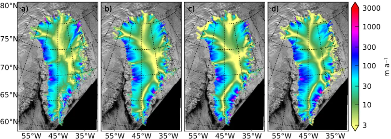
Consequences of a warmer climate on the Greenland Ice Sheet (GrIS) mass balance will be a thickening inland, due to increased solid precipitation, and a thinning at the GrIS

indicate our constraints: error values < 20 % for ice thickness, a 45 to 65 % range for mass balance partition and an Eemian to present-day surface elevation reduction of ≤ 430 m

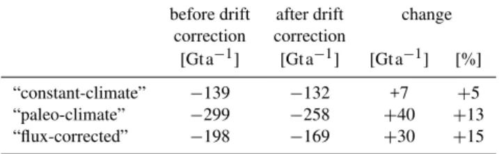
(1998) is typical, it yields a loss rate of 0.14 % a − 1 if applied to the whole Greenland ice perimeter divided by Greenland ice area, or 0.006 % a − 1 if applied to the

Northern Hemisphere ice sheets simulated by the GRISLI model at 18 ka BP, prior to Heinrich event 1, in terms of ice thickness (a) , ice velocities (b) and subsurface (550–1050 m)