TCD
8, 1151–1189, 2014Greenland ice sheet simulations
R. Calov et al.
Title Page
Abstract Introduction
Conclusions References
Tables Figures
◭ ◮
◭ ◮
Back Close
Full Screen / Esc
Printer-friendly Version Interactive Discussion
Discussion
P
a
per
|
D
iscussion
P
a
per
|
Discussion
P
a
per
|
Discuss
ion
P
a
per
The Cryosphere Discuss., 8, 1151–1189, 2014 www.the-cryosphere-discuss.net/8/1151/2014/ doi:10.5194/tcd-8-1151-2014
© Author(s) 2014. CC Attribution 3.0 License.
Open Access
The Cryosphere
Discussions
This discussion paper is/has been under review for the journal The Cryosphere (TC). Please refer to the corresponding final paper in TC if available.
Simulating the Greenland ice sheet under
present-day and palaeo constraints
including a new discharge
parameterization
R. Calov1, A. Robinson1,2,3, M. Perrette1, and A. Ganopolski1
1
Potsdam Institute for Climate Impact Research, Potsdam, Germany
2
Universidad Complutense Madrid, 28040 Madrid, Spain
3
Instituto de Geociencias, UCM-CSIC, 28040 Madrid, Spain
Received: 22 January 2014 – Accepted: 4 February 2014 – Published: 17 February 2014 Correspondence to: R. Calov ([email protected])
TCD
8, 1151–1189, 2014Greenland ice sheet simulations
R. Calov et al.
Title Page
Abstract Introduction
Conclusions References
Tables Figures
◭ ◮
◭ ◮
Back Close
Full Screen / Esc
Printer-friendly Version Interactive Discussion
Discussion
P
a
per
|
D
iscussion
P
a
per
|
Discussion
P
a
per
|
Discuss
ion
P
a
per
|
Abstract
In this paper, we propose a new sub-grid scale parameterization for the ice discharge into the ocean through outlet glaciers and inspect the role of different observational and palaeo constraints for the choice of an optimal set of model parameters. This param-eterization was introduced into the polythermal ice-sheet model SICOPOLIS, which is 5
coupled to the regional climate model of intermediate complexity REMBO. Using the coupled model, we performed large ensemble simulations over the last two glacial cy-cles. We exploit two major parameters: a melt parameter in the surface melt scheme of REMBO and an ice discharge parameter in our parameterization of ice discharge. Our constraints are the present-day Greenland ice sheet surface elevation, surface mass 10
balance partition (ratio between ice discharge and total precipitation) and the Eemian interglacial elevation drop relative to present-day in the vicinity of the NEEM ice core. We show that the ice discharge parameterization enables us to simulate both the cor-rect ice-sheet shape and mass balance partition at the same time without explicitly resolving the Greenland outlet glaciers. For model verification, we compare simulated 15
total and sectoral ice discharge with those from other findings, including observations. For the model versions, which are inside the range of observational and palaeo con-straints, our simulated Greenland ice sheet contribution to Eemian sea level rise rela-tive to present-day amounts to 1.4 m on average (in the range of 0.6 and 2.5 m).
1 Introduction 20
Modelling the response of the Greenland Ice Sheet (GIS) to anthropogenic warming has already been undertaken for more than two decades (Huybrechts et al., 1991; van de Wal and Oerlemans, 1997; Huybrechts and de Wolde, 1999; Greve, 2000) and attracted considerable attention in recent years (Vizcaíno et al., 2010; Goelzer et al., 2011; Graversen et al., 2011; Applegate et al., 2012; Lipscomb et al., 2013; Stone et al., 25
TCD
8, 1151–1189, 2014Greenland ice sheet simulations
R. Calov et al.
Title Page
Abstract Introduction
Conclusions References
Tables Figures
◭ ◮
◭ ◮
Back Close
Full Screen / Esc
Printer-friendly Version Interactive Discussion
Discussion
P
a
per
|
D
iscussion
P
a
per
|
Discussion
P
a
per
|
Discuss
ion
P
a
per
Seddik et al., 2012; Goelzer et al., 2013). The recent SeaRISE ice sheet modelling project (Nowicki et al., 2013) highlighted the importance of treatment of processes at the ice-ocean interface for the response of models of the Greenland ice sheet to future climate change.
Observational data indicate that during the past decade mass loss by the GIS, both 5
through surface melt and enhanced ice discharge, has contributed appreciably to global sea level rise (Shepherd et al., 2012). The latest projections suggest that the GIS will contribute notably to sea level rise during the next century (Hanna et al., 2013). In the longer-term perspective, the GIS can become even more important, because even if the global temperature is stabilised at the level of 2◦C above preindustrial, the GIS 10
would still continue to melt and, in the long-term perspective, can lose a significant fraction of its mass even for moderate warming (Ridley et al., 2005; Robinson et al., 2012).
Models of the GIS contain a number of parameters, which can be used for tuning the model using observational constraints. Present-day extent and surface elevation of the 15
GIS are accurately known and it is natural to use them as such constraints (e.g. Stone et al., 2010; Greve et al., 2011; Lipscomb et al., 2013). At the same time, it is known that coarse-resolution ice-sheet models have problems in simulating the correct margins of the GIS and they systematically overestimate its volume. One reason is that under present-day conditions, most ice discharge into the ocean occurs through relatively 20
narrow outlet glaciers. As a result, although ice discharge into the ocean currently accounts for more than half of surface accumulation, over most of Greenland the ice sheet margin is located several tens of kilometres away from the ocean. Since current ice-sheet models do not resolve outlet glaciers and their interaction with the ocean in the fjords, the modelled GIS needs too much contact with the ocean to produce 25
realistic discharge. This leads to systematic overestimation of the ice area and volume and makes observational “geometrical” constraints difficult to apply.
TCD
8, 1151–1189, 2014Greenland ice sheet simulations
R. Calov et al.
Title Page
Abstract Introduction
Conclusions References
Tables Figures
◭ ◮
◭ ◮
Back Close
Full Screen / Esc
Printer-friendly Version Interactive Discussion
Discussion
P
a
per
|
D
iscussion
P
a
per
|
Discussion
P
a
per
|
Discuss
ion
P
a
per
|
mass balance partition (defined as the ratio between ice discharge into the ocean and total precipitation over the GIS, MBP) as another constraint on the GIS. The MBP is an important characteristic for short-term as well as for long-term (future) behaviour of the GIS, because it determines the GIS mass balance sensitivity to climate change. In particular, the present-day MBP is related to the long-term stability properties of the 5
GIS (Robinson et al., 2012), i.e. for low MBP values (large surface melt) the modelled GIS is more susceptible to warming than for high ones. For the long-term stability of the GIS, the MBP is a more important characteristic than the present-day shape of the GIS. However for short-term (centennial time scale) future global warming simulations, such an ice sheet would be an unfavourable initial condition, because during a consid-10
erable portion of time of such a future simulation the modelled ice would melt in areas, where in reality no ice exists (Goelzer et al., 2013). Since standard coarse-resolution GIS ice sheet models cannot simulate a realistic present-day extent/surface orography of the GIS and at the same time have the correct mass balance partition, we devel-oped a novel approach, which allows us to circumvent this problem, without resolving 15
individual ice streams and outlet glaciers – and without an increase in computational cost. This approach is in the spirit of our previous modelling work (Robinson et al., 2010, 2011, 2012) and is based on a rather simple semi-empirical parameterization of ice discharge through the outlet glaciers. We propose the usage of this approach until a more complete representation of fast processes is available. Considering the above 20
concerns, this approach is feasible for short-term as well as for long-term simulations. In addition to the present-day constraints on the ice-sheet shape and the MBP, we use the Eemian as a palaeo constraint. Eemian conditions have already been recog-nized earlier as an important palaeo constraint for GIS model parameters (Tarasov and Peltier, 2003) and have been applied more recently in several studies (Robinson 25
TCD
8, 1151–1189, 2014Greenland ice sheet simulations
R. Calov et al.
Title Page
Abstract Introduction
Conclusions References
Tables Figures
◭ ◮
◭ ◮
Back Close
Full Screen / Esc
Printer-friendly Version Interactive Discussion
Discussion
P
a
per
|
D
iscussion
P
a
per
|
Discussion
P
a
per
|
Discuss
ion
P
a
per
climate changes during Eemian (Born and Nisancioglu, 2012). In the present paper, we make use of the recently published estimate of the Eemian elevation drop at a position of about 200 km upstream of NEEM (NEEM community members, 2013), where the borehole ice sampled today was deposited during Eemian.
The paper is summarized as follows. First, we give a short description of the ice-5
sheet model SICOPOLIS and the regional energy-moisture balance model REMBO (Sect. 2). Our new discharge parameterization is comprehensively explained in Sect. 3. Different metrics of model performance are introduced and discussed in Sect. 4. In Sect. 5, we describe our constraints and simulations and compare our findings with those of others, as well as with observations. We close with a discussion and finally 10
our conclusions.
2 Model description
For this study, we used the three-dimensional polythermal ice-sheet model SICOPO-LIS (version 2.9) coupled to the regional energy-moisture balance model (REMBO). SICOPOLIS treats the evolution of ice thickness, ice temperature and water content 15
(Greve, 1997) based on the shallow ice approximation. The dependence of the ice ve-locities on the ice temperature and water is introduced via the rate factor. SICOPOLIS enables a free and easy choice of several parameters including resolution. In our pa-per, Greenland is mapped onto a stereographic plane with 76×141 grid points (20 km grid spacing) using the topographic dataset by Bamber et al. (2001). The vertical is re-20
solved by 90 layers with decreasing layers thickness towards the bed of the ice sheet. A 10-layer thermal rock bed is coupled to the overlying ice sheet via heat fluxes. The geothermal heat flux is prescribed at the lower border of the thermal bedrock. The bedrock adjusts to the load caused by the ice sheet’s weight using a local lithosphere relaxing asthenosphere model with a time delay of 3000 yr.
25
TCD
8, 1151–1189, 2014Greenland ice sheet simulations
R. Calov et al.
Title Page
Abstract Introduction
Conclusions References
Tables Figures
◭ ◮
◭ ◮
Back Close
Full Screen / Esc
Printer-friendly Version Interactive Discussion
Discussion
P
a
per
|
D
iscussion
P
a
per
|
Discussion
P
a
per
|
Discuss
ion
P
a
per
|
diffusion-type equations for surface air temperature and atmospheric water content. For temperature, the well-known Budyko–Sellers energy balance approach is imple-mented. Planetary albedo is related to surface albedo via a linear parameterization based on empirical data. The lateral boundary conditions for temperature and rela-tive humidity are taken from climatology (Uppala et al., 2005) for the years 1958–2001, 5
which in this paper is referred to as “present-day”. REMBO includes a 1-layer snowpack model with a simple parameterization of refreezing. Surface albedo depends on snow thickness and the melt rate. Surface melt is computed using a simple parameterization of van den Berg et al. (2008) and depends on both temperature and insolation. The formula for surface melt contains a free parametercm (melt parameter), which is one 10
of the major parameters determining the sensitivity of the ice sheet to climate change (Robinson et al., 2011). It reads
m= ∆t
ρwLm
[τs(1−αs)S+cm+λT], (1)
which relates the potential surface meltmwith the free melt parametercm. The
remain-ing variables∆t,ρw,Lm,τs,αs,S,λand T, are the day length, the density of water,
15
the latent heat of ice melting, the total transmissivity, the surface albedo, the insola-tion at the top of the atmosphere, the long wave radiainsola-tion coefficient and the surface temperature, respectively. Please, refer to (Robinson et al., 2011) for more details.
The coupling between the models is bi-directional, i.e., SICOPOLIS provides the climate model with information about surface elevation and spatial extent of the ice 20
sheet. In turn, REMBO provides SICOPOLIS with surface mass balance and mean annual surface temperature.
3 Ice discharge parameterization
TCD
8, 1151–1189, 2014Greenland ice sheet simulations
R. Calov et al.
Title Page
Abstract Introduction
Conclusions References
Tables Figures
◭ ◮
◭ ◮
Back Close
Full Screen / Esc
Printer-friendly Version Interactive Discussion
Discussion
P
a
per
|
D
iscussion
P
a
per
|
Discussion
P
a
per
|
Discuss
ion
P
a
per
discharge into the ocean is parameterized as
d=ch
p
lq, defined over∆R, (2)
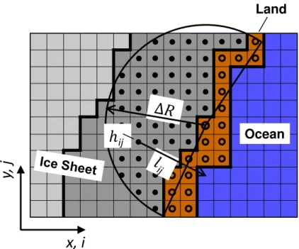
where l and h are the distance from the actual grid cell (i,j) to the nearest ocean grid cell and the ice thickness, respectively. They are the two major variables, which control the ice discharge. The parameterization applies to any grid point located within 5
a distance∆R from the nearest ice-free land surface points (note∆R only determines whether the parameterization applies or not, but plays no role for the actual value of the discharge; see Fig. 1 for an illustration).
The parametercvaries strongly for different values of the powerspandqto maintain constant discharge. For convenience, we normalizecas
10
c=c0cd, (3)
i.e., for any fixed value ofpandqwe selectedc0such thatcdhas a value of about one.
In practice, after selectingp andq we chose c0so that the parameterization applied
to observed Greenland elevation matched observed total discharge, for which we used 350 Gt yr−1. The latter value is just about the average of the totals of ice discharge as 15
found by Reeh (1994) and (Rignot et al., 2008). Although the discharge for the modelled present-day GIS will not be precisely 350 Gt yr−1, such an approach guarantees that all valid values of the parametercdmaintain the order of magnitude of about one for any
powerpandq.
We thus have three free ice-discharge parameterscd,pandqin our
parameteriza-20
tion (Eqs. 2 and 3). Based on an ensemble of model simulations, we chosep=1 and
q=3 for the powers, and the range of valid cd was selected using the observational constrains as it is described below (Sect. 5.1). For the above powers, we fix the de-pendent parameter asc0=2.61×10
4
m3s−1. Both the discharge parametercdand the
melt parametercmdetermine the major characteristics of the GIS. Therefore, a set of
25
TCD
8, 1151–1189, 2014Greenland ice sheet simulations
R. Calov et al.
Title Page
Abstract Introduction
Conclusions References
Tables Figures
◭ ◮
◭ ◮
Back Close
Full Screen / Esc
Printer-friendly Version Interactive Discussion
Discussion
P
a
per
|
D
iscussion
P
a
per
|
Discussion
P
a
per
|
Discuss
ion
P
a
per
|
Additionally, we assume that ice discharge only occurs if the inland-ice surface is descending toward the coast. This is enforced by setting a maximum value ofα0=60
◦
to the angle between the gradients of surface elevation∇zsand distance field∇l (see
Fig. 2 for the characteristics of the fieldl). Using the definition of the scalar product for the angle between above two gradients this reads
5
∇zs·∇l
|∇zs||∇l|≥cos(α0), evaluated at (i,j). (4)
This prevents our parameterization from simulating ice discharge into the ocean from an ice margin, which is oriented towards the interior of the Greenland island, which could happen when the GIS is retreating under warm climates and only a few small ice sheets remain, see the small land bridge between the two ice caps in Fig. 3b for 10
example.
The discharge parameterization is applied only to the ice covered grid cells which are located not more than ∆R (here ∆R=120 km) from the ice margin (see Fig. 1). The resulting belt encloses the regions of ice with rather high velocities as found by satellite measurements (Joughin et al., 2010; Rignot and Mouginot, 2012). The idea 15
here is to largely capture two aspects of fast ice flow with this parameterization: the fast outlet glaciers themselves, as well as the rather fast flowing ice in the catchment regions upstream of the outlet glaciers. The ice thickness hdescribes the amount of ice that can be brought to the outlet glaciers. And the power of the inverse distance to the coast (1/l)q can be regarded as a statistical measure of the outlet glacier density: 20
if the ice margin is far away from the coast, it is very unlikely that any outlet glacier has contact with the ocean and there is only minor calving flux into the ocean, while one would expect a large calving flux for small distances to the coast.
Although the parameterization by Eq. (2) mimics non-resolved lateral ice discharge, the term d has the dimension m s−1. The term is directly included in the evolution 25
equation of ice thickness evolution as
∂h
TCD
8, 1151–1189, 2014Greenland ice sheet simulations
R. Calov et al.
Title Page
Abstract Introduction
Conclusions References
Tables Figures
◭ ◮
◭ ◮
Back Close
Full Screen / Esc
Printer-friendly Version Interactive Discussion
Discussion
P
a
per
|
D
iscussion
P
a
per
|
Discussion
P
a
per
|
Discuss
ion
P
a
per
whereqand b are the lateral mass flux and the surface mass balance, respectively. Unlike the surface mass balance, the ice discharged in our model depends only on the ice-sheet geometry.
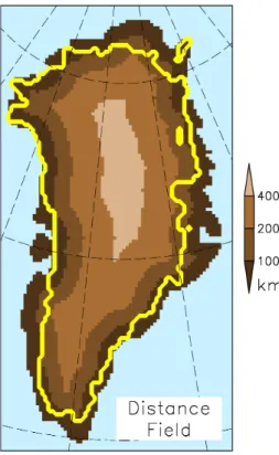
As seen in Fig. 2, the minimal distance to the coastl can reach up to about 400 km in the centre of Greenland. In our parameterization, the inverse dependence of the ice 5
discharge on the minimal distance to the coast – here even to the third power – is a condition for high ice discharge over regions with small minimal distance (dark brown colour) and low discharge further inland (lighter brown colours). For a minimal distance of around 400 km the parameterized ice discharge would nearly vanish. In our dis-charge parameterization, this is relevant for an ice sheet under warmer climates, which 10
can be smaller than the present-day GIS. Recall that our parameterization only applies for∆R <120 km around the ice margins. One can see that the observed present-day Greenland near-margin ice area largely covers regions with small minimal distances. These are the regions where a high present-day ice discharge due to many outlet glaciers is observed (e.g. Moon et al., 2012), e.g. over the north-western region of the 15
GIS. For regions with fewer marine outlet glaciers, e.g. in the south-west, the observed ice margin resides rather in regions with larger minimal distances.
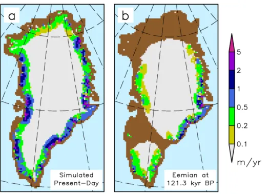
As stated above, our discharge parameterization is not intended to resolve every small individual outlet glacier; it is rather designed to capture their draining effect on spatial and temporal average in a sub-grid scale statistical approach. In general, our 20
simulated present-day ice discharge (Fig. 3a) is high over regions with many observed outlet glaciers and low over regions with fewer observed outlet glaciers, see Fig. 3 in Moon and Joughin (2008) for comparison. However, in the south-western part of Greenland we overestimate the ice discharge, in part due to too high simulated accu-mulation over that region (compare Sect. 5.3).
25
TCD
8, 1151–1189, 2014Greenland ice sheet simulations
R. Calov et al.
Title Page
Abstract Introduction
Conclusions References
Tables Figures
◭ ◮
◭ ◮
Back Close
Full Screen / Esc
Printer-friendly Version Interactive Discussion
Discussion
P
a
per
|
D
iscussion
P
a
per
|
Discussion
P
a
per
|
Discuss
ion
P
a
per
|
and fjords. In particular, this means if our parameterized ice discharge is strong – i.e., the validcd is sufficiently large –, then there is practically no explicit SICOPOLIS ice
discharge, since GIS is not in direct contact with the ocean in this case. It can be seen that for large distances of the ice margin to the coast there is less ice discharge than for small distances, as intended with our parameterization.
5
4 Measures of geometrical characteristics of an ice sheet
There are numerous possibilities to define a measure of the performance of a model based on the comparison of simulated geometrical characteristics of an ice sheet with observational data. The simplest is to use the error in simulated total ice area and ice volume, which we define as
10
err(A)=|Amod−Aobs|
Aobs
·100, err(V)=|Vmod−Vobs|
Vobs
·100, (6)
where Aobs, Amod, Vobs and Vmod are the observed ice area, the modelled ice area,
the observed ice volume and the modelled ice volume, respectively. These errors in principle can approach zero, but this does not guarantee accurate simulation of the ice-sheet geometry, since regional errors can compensate each other. Therefore, we 15
choose a stronger constraint based on the error in ice thickness expressed relatively to the total ice thickness. This reads
err(H)= P
i j|H
mod
i j −H
obs
i j | P
i jHi jobs
·100, (7)
whereHi jobs and Hi jmod are, respectively, the observed and measured ice thickness at the horizontal grid position (i,j). The indicesi,jrun over the entire domain of the com-20
TCD
8, 1151–1189, 2014Greenland ice sheet simulations
R. Calov et al.
Title Page
Abstract Introduction
Conclusions References
Tables Figures
◭ ◮
◭ ◮
Back Close
Full Screen / Esc
Printer-friendly Version Interactive Discussion
Discussion
P
a
per
|
D
iscussion
P
a
per
|
Discussion
P
a
per
|
Discuss
ion
P
a
per
This error only approaches zero when the ice-sheet thickness is correctly simulated in each grid cell.
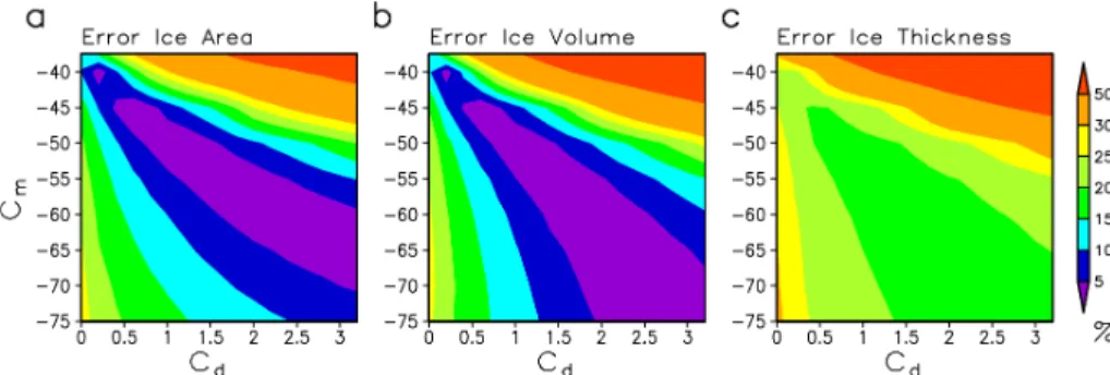
Figure 4 compares the three error measures for the ice-sheet shape in the phase space of the melt, cm, and discharge, cd, parameters. At first sight, the error fields
in the three panels look similar. The smallest errors appear approximately along the 5
descending diagonal, which is characterised by decreasing values ofcmand increasing
values of cd. One can also see that the parameter combinations with small errors
are not limited to our sampled space: these regions expand in the direction of the descending diagonal. This underlines the need for more constraints (Sect. 5.1).
Figure 4 illustrates that our discharge parameterization allows us to reduce the errors 10
in total area and volume practically to zero. However, we found no parameter combi-nation for which the error in ice thickness was much lower then 20 %. Still, these are considerable improvements compared to standard version of the model without ice discharge parameterization constrained only by the mass balance partition (Robinson et al., 2011), which overestimates total ice volume and area by ca. 20 % and has a rel-15
ative thickness error of ca. 30 %. When the mass balance partition is ignored, one can improve model performance by increasing surface melt. By choosingcm=−40 W m−2,
one can make all three errors comparable with those of the best model version with ice discharge parameterization. However, such a high melt factor practically eliminate ice discharge into the ocean and, as shown below, drastically affects the GIS stability. In 20
fact, it causes the GIS to be unstable even under near present-day climate conditions.
5 Results
5.1 Model setup and constraints
Following Robinson et al. (2011), we run the coupled REMBO-SICOPOLIS model through two glacial cycles starting at 250 kyr BP. These simulations serve a dual pur-25
TCD
8, 1151–1189, 2014Greenland ice sheet simulations
R. Calov et al.
Title Page
Abstract Introduction
Conclusions References
Tables Figures
◭ ◮
◭ ◮
Back Close
Full Screen / Esc
Printer-friendly Version Interactive Discussion
Discussion
P
a
per
|
D
iscussion
P
a
per
|
Discussion
P
a
per
|
Discuss
ion
P
a
per
|
GIS and to apply palaeoclimate constraints (see below) to additionally reduce the range of model parameters. To drive the model through two glacial cycles, we apply variations in insolation due to changes in orbital parameters, CO2concentration and regional
tem-perature anomaly obtained from the CLIMBER-2 model (Petoukhov et al., 2000; Calov et al., 2005). We took these anomalies from the standard simulation as in Ganopol-5
ski and Calov (2011). To generate an ensemble of model realisations, we vary two parameters: the discharge parametercd(Sect. 3) and the melt parametercm. The dis-charge parameter cd is varied in steps of 0.2 and the melt parameter cm in steps of
5 W m−2. The geothermal heat flux is set to 50 mW m−2 and the sliding coefficient to 15 m (yr Pa)−2. All other parameters are the same as in Robinson et al. (2010).
10
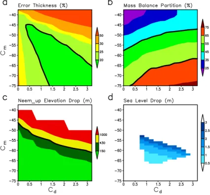
As constraints on the ensemble, we use the relative error in present-day ice thickness (see Sect. 4), the present-day surface mass balance partition and the Eemian drop in surface elevation relative to present-day upstream of the ice borehole position NEEM. Figure 5a–c illustrates all constraints used in this paper.
We accept a value of 20 % for the error in ice thickness. This choice is not totally 15
arbitrary, because a closer inspection of the error field shows a minimum error in ice thickness of 18.2 %, i.e., there is indeed a plateau defined by ice thickness error values
≤20 %, as illustrated in Fig. 5a by the medium green shading. Within the parameter space, the error in ice thickness varies much more strongly for values higher than 20 %. This supports the latter value as a reasonable constraint for the determination of valid 20
parameters.
As mentioned in the introduction, the mass balance partition is the amount of ice discharge compared to precipitation. In our work, we always refer to MBP as a char-acteristic of the ice sheet defined in its present-day state. Its practical definition is the total ice discharge divided by the total precipitation for the simulated present-day ice 25
TCD
8, 1151–1189, 2014Greenland ice sheet simulations
R. Calov et al.
Title Page
Abstract Introduction
Conclusions References
Tables Figures
◭ ◮
◭ ◮
Back Close
Full Screen / Esc
Printer-friendly Version Interactive Discussion
Discussion
P
a
per
|
D
iscussion
P
a
per
|
Discussion
P
a
per
|
Discuss
ion
P
a
per
operate with the simulated present day ice-sheet topography for determining MBP, be-cause of the better match between simulated and observed topography. This means that our new MBP values simulated with ice discharge parameterization slightly differ from our former approach (cd=0), and the valid MBP range (Fig. 5b) corresponds
to somewhat lower values ofcm compared to those by Robinson et al. (2011).
How-5
ever, the MBP has large inherent uncertainty, which we derived from regional climate models, following Robinson et al. (2011) and yielding a range of 45 % to 65 %.
From measurement of air content in the NEEM borehole samples, the NEEM com-munity members (2013) found that the surface elevation was 130±300 m lower during Eemian than at present-day, which we exploit as our third constraint. Following these 10
findings, we assume the maximal surface elevation drop at this location during Eemian (130 to 115 kyr BP) did not exceed 430 m (compared to present-day). Accounting for the trajectory tracing results by NEEM community members (2013), we used the de-position de-position of NEEM, a location about 200 km upstream from NEEM at (45◦W, 76◦N) (see Fig. 7d), denoted NEEMup hereafter. This upstream position is the location 15
where the sampled NEEM ice was deposited by snowfall during Eemian, carrying the air composition at that upstream position, which therefore is the location at which the Eemian change in surface elevation happened.
Figure 5a–c illustrates that none of the constraints is redundant, because the regions of valid simulations for all three constraints intersect each other and there is plenty 20
of space without a common crossover for every constraint. In particular, the error in thickness excludes low values of the ice discharge parameter, while the mass balance partition constrains the range of the melt parameter, the upper bound of which is then further constrained by the NEEMup elevation data. While the valid region of all three constraints cover an about equally large part of the parameter space (Fig. 5a–c), only 25
a relatively small subset of model parameters (Fig. 5d) is consistent with all of these constraints simultaneously.
TCD
8, 1151–1189, 2014Greenland ice sheet simulations
R. Calov et al.
Title Page
Abstract Introduction
Conclusions References
Tables Figures
◭ ◮
◭ ◮
Back Close
Full Screen / Esc
Printer-friendly Version Interactive Discussion
Discussion
P
a
per
|
D
iscussion
P
a
per
|
Discussion
P
a
per
|
Discuss
ion
P
a
per
|
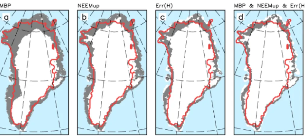
band of valid ice margins, while the NEEMup constraint (Fig. 6b) alone results in an ice margin range, which is quite comparable with that of the err(H) constraint (Fig. 6c). Finally, all three constraints together give a pronounced reduction of spread of ice mar-gins (Fig. 6d) compared to the single-constraint cases. Simulated ice marmar-gins in the south, mid-west and northeast of Greenland compare well with observations. How-5
ever, there are regions with rather strong mismatch in the southwest and in the north. Parts of this mismatch can be attributed to our model biases in precipitation. For exam-ple, REMBO simulates too much snow accumulation in the northeast and southwest of Greenland compared to the compilation by Bales et al. (2009).
Figure 5d depicts the simulated difference in GIS volume between Eemian and 10
present-day expressed in units of global sea level. Compared to the other figure pan-els, we show here results from simulations with the refined melt parameter spacing of 1 W m−2. We enhanced the resolution of the melt parameter sampling, because the region of valid simulations appears rather elongated in the parameter space. The es-timated Eemian sea level contribution increases with increasing values ofcm. This is
15
understandable, because surface melting increases with larger melt parameter values. Nevertheless, there is also an increase of the GIS contribution to the Eemian sea-level highstand for increasing discharge parameter values. Obviously, there is an interplay between ice discharge and surface melt, because the ice discharge removes ice from the ice sheet and brings the ice surface into lower regions of the atmosphere, where 20
stronger surface melt can occur. Averaged over the parameter space of valid simula-tions, we have a contribution of the GIS to Eemian sea level rise (above present-day value) of 1.4 m. The minimum contribution of the GIS sea level rise among all valid simulations is 0.6 m and the corresponding maximum is 2.5 m.
5.2 Eemian vs. present-day and GIS stability 25
TCD
8, 1151–1189, 2014Greenland ice sheet simulations
R. Calov et al.
Title Page
Abstract Introduction
Conclusions References
Tables Figures
◭ ◮
◭ ◮
Back Close
Full Screen / Esc
Printer-friendly Version Interactive Discussion
Discussion
P
a
per
|
D
iscussion
P
a
per
|
Discussion
P
a
per
|
Discuss
ion
P
a
per
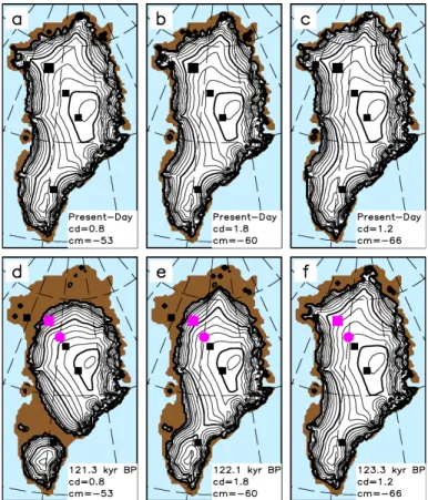
there is a considerable difference between the corresponding Eemian fields. However, the present-day surface elevations for the different valid parameters sets still show slight differences. Naturally, these differences appear mainly near the ice margin, while the interior of the ice sheet remains almost unchanged for any valid parameter set. As is often the case in such optimization problems, there is a trade-offconcerning agreement 5
with observations in certain regions (see Fig. 9a for the observed surface elevation). While the simulation withcd=0.8,cm=−53 W m−2 (Fig. 7a) better resembles the ice-free southwestern region, the northern region around Petermann Gletscher matches the observation less well. This situation is opposite for the simulation with cd=1.2, cm=−66 W m−2(Fig. 7c).
10
For all valid parameter sets, our simulated reduction in Eemian ice volume is accom-panied by a strong retreat of ice in Greenland in particular in its northern part, see Fig. 7d–f, which spans simulated lowest and highest Eemian to present-day GIS con-tribution to sea level drop. For model versions with high sensitivity to climate forcing, the GIS splits into two parts: a small ice cap in southern Greenland and a larger ice 15
sheet in central Greenland (Fig. 7d). For the intermediate and low sensitivity model versions, the GIS remains in one piece (Fig. 7e and f). In all valid model versions, there is a strong retreat of ice, mainly in western and northern Greenland. Our estimates showing a strong retreat of the GIS during Eemian rather correspond to the simula-tions by Otto-Bliesner et al. (2006), while the medium to modest retreat of the Eemian 20
GIS was found in simulations by Helsen et al. (2013) and Quiquet et al. (2013).
Interestingly, the NEEM location almost becomes ice free at 121 kyr BP in our most sensitive model version, see Fig. 7d. Nonetheless, an ice free NEEM position dur-ing Eemian would not contradict the existence of Eemian ice and most probably pre-Eemian ice in the NEEM ice core at present-day, as reported by NEEM community 25
members (2013), since the Eemian ice was accumulated farther upstream of NEEM. Similar argumentation would hold for Camp Century as well.
TCD
8, 1151–1189, 2014Greenland ice sheet simulations
R. Calov et al.
Title Page
Abstract Introduction
Conclusions References
Tables Figures
◭ ◮
◭ ◮
Back Close
Full Screen / Esc
Printer-friendly Version Interactive Discussion
Discussion
P
a
per
|
D
iscussion
P
a
per
|
Discussion
P
a
per
|
Discuss
ion
P
a
per
|
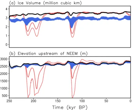
(Robinson et al., 2011) and our present approach, which includes the sub-grid scale discharge parameterization. At all times, the valid model versions with the discharge parameterization simulate less ice volume than that without the discharge parameter-ization (Fig. 8a). This has two reasons: (i) previously, the model was not tuned for agreement with present-day surface elevation (ice volume). The present-day surface 5
mass balance partition was (and is here) regarded as the more adequate characteris-tic to capture the sensitivity of the GIS to long-term climate change. (ii) In our present approach, the inclusion of the discharge parameterization enables our rather coarse resolution model to mimic the calving of the small-scale outlet glaciers (i.e. removal in ice into the ocean by ice discharge) without an overestimation of contact regions of the 10
ice sheet with the ocean, which leads to a smaller ice sheet.
Additionally, two extreme and unrealistic simulations, depicted by the red lines, were set up in order to demonstrate, what happens when a shape-only tuning applies in a coarse-resolution model, which disregards fast sub-grid processes of small outlet glaciers. Technically, we restrict the parameter space by settingcd=0 (discharge
pa-15
rameterization off) and minimize the error measure err(H) and, alternatively, the weaker error measure err(V) to get the right present-day shape. The former belongs to the parameter setting cd=0, cm=−42 W m−2 and the latter to cd=0, cm=−40 W m−2.
Please, note that these melt parameter values are outside the valid range of MBP as determined by Robinson et al. (2011) using observed present-day topography as well 20
as outside the valid cm values in MBP space of this work (Fig. 5b) using simulated
present-day topography to determine MBP. Because we consider the present-day ice-sheet shape as the only constraint (for demonstration), the model without the discharge parameterization (cd=0) appears to perform well in thecmspace, but the melt
param-etercmbecomes rather high for all minimized shape errors (Fig. 4). As one can see in
25
TCD
8, 1151–1189, 2014Greenland ice sheet simulations
R. Calov et al.
Title Page
Abstract Introduction
Conclusions References
Tables Figures
◭ ◮
◭ ◮
Back Close
Full Screen / Esc
Printer-friendly Version Interactive Discussion
Discussion
P
a
per
|
D
iscussion
P
a
per
|
Discussion
P
a
per
|
Discuss
ion
P
a
per
different model versions. However, during the Eemian interglacial, the runs from the shape-only constraints show strong downward excursions for ice volume as well as for the NEEMup elevation (Fig. 8b). Whether such a small Eemian ice volume is still realistic might be disputable. Nevertheless, the Eemian reduction in NEEMup eleva-tion is by far larger than that estimated from the ice core (NEEM community members, 5
2013). The Eemian NEEMup position was even ice free in the shape-only simulation with minimized err(V), which certainly contradicts observational data.
Moreover, the strong drop in Eemian sea level and NEEMup elevation hints at very different stability properties of the model version with shape-only tuning in a coarse resolution model compared to all our valid model versions, which are still on coarse res-10
olution, but contain our sub-grid scale discharge parameterization. Namely, the models with shape-only tuning are much more unstable than all the model versions that are constrained using the MBP and palaeo data. Most important, both of our sets of model versions are more stable than those models with shape-only tuning of melt parameter: the valid model versions of our former approach without discharge parameterization 15
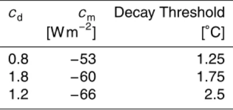
(Robinson et al., 2011, 2012) as well as our present ones with discharge parameter-ization. To achieve more meaningful information about the stability of the system, we performed an analysis based on many steady state runs over 300 kyr as in Calov and Ganopolski (2005), but in temperature space instead of insolation space. From those simulations, we obtain thresholds of decay of the GIS between 1.25◦C and 2.5◦C for 20
the model versions with the discharge parameterization, depending on the position in parameter space (see also Table 1). The threshold estimated with the shape-only set-ting with err(V) minimisation (cd=0, cm=−40 W m
−2
) is much lower – only 0.25◦C. The higher values for GIS decay between 1.25◦C and 2.5◦C from our new REMBO-SICOPOLIS version with discharge parameterization are in the range of those that 25
TCD
8, 1151–1189, 2014Greenland ice sheet simulations
R. Calov et al.
Title Page
Abstract Introduction
Conclusions References
Tables Figures
◭ ◮
◭ ◮
Back Close
Full Screen / Esc
Printer-friendly Version Interactive Discussion
Discussion
P
a
per
|
D
iscussion
P
a
per
|
Discussion
P
a
per
|
Discuss
ion
P
a
per
|
in Sect. 5.1. It should be noted that a complete uncertainly analysis with our new model version is planned in the future, which will likely widen the range of our estimates.
In summary, whether we optimize the melt parameter in the coarse resolution model for err(H) or err(V), the resulting simulations all violate the MBP criterion. This leads to a strong drop of the NEEM elevation far below the one reconstructed from palaeo 5
data, and the Greenland ice sheet becomes too instable. This is why (Robinson et al., 2011) and (Robinson et al., 2012) used the MBP criterion together with a palaeo con-straint for calibration of their coarse resolution model, ensuring the correct long-term stability properties reported in this work. In our improved model with sub-grid scale discharge parameterization, we found a stability behaviour similar to that by Robin-10
son et al. (2012) when using the MBP and NEEMup constraints, but now – still in the coarse resolution ice-sheet model – we can additionally fulfil a strong present-day shape constraint (err(H)<20 %). We expect that all our constraints will play a similar role in a model of the Greenland glacial system which explicitly describes small-scale fast processes. Development of such a model is in our future plans.
15
One major advantage of our simple parameterization is that it applies easily for climates far away from present-day – a fully explicit modelling of present-day outlet glaciers could break down for the Eemian, because many present-day outlet glaciers just vanish in the Eemian. Figure 3a and b compares simulated ice discharge during present-day and Eemian. The present-day ice-discharge field was discussed already 20
in Sect. 3. Here, we demonstrate that the regions of fast flow can reduce drastically for the Eemian time period compared to the present-day state. For the Eemian, there is practically no ice discharge over regions far away from the coast. In particular, the land bridge between the large ice sheet in the north and the smaller ice cap in the south of Greenland shows vanishing ice discharge. In general, our model results suggest that 25
TCD
8, 1151–1189, 2014Greenland ice sheet simulations
R. Calov et al.
Title Page
Abstract Introduction
Conclusions References
Tables Figures
◭ ◮
◭ ◮
Back Close
Full Screen / Esc
Printer-friendly Version Interactive Discussion
Discussion
P
a
per
|
D
iscussion
P
a
per
|
Discussion
P
a
per
|
Discuss
ion
P
a
per
5.3 Comparison with present-day observations and findings by others
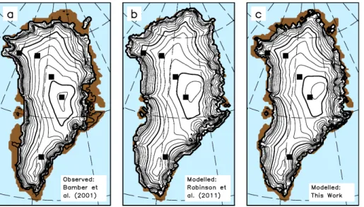
A direct comparison of our simulated Greenland surface elevation with the observed elevation by Bamber et al. (2001) and the former approach of Robinson et al. (2010) is shown in Fig. 9. Overall, we improved agreement with observations significantly. In par-ticular, in the simulation with the discharge parameterization several regions are now 5
ice-free, which look very similar to reality. The remaining deficiencies are partly due to the simple discharge parameterization and the limitations in the REMBO climatology, e.g., biases in representation of precipitation as discussed earlier. In this context, we would like to stress, that our model is a fully interactive one, where no observational data over Greenland are prescribed. This ensures that REMBO is applicable to cli-10
mates far away from the present state, what is vital because the Eemian climate can deliver additional constraints for the model.
Figure 10 compares our simulated present-day sectoral and total ice discharge with findings by others. The sectors (see inset in the upper right of Fig. 10) corre-spond with those of Reeh (1994) and sub-divide the GIS into a northern (sector N), 15
north-western (sector NW), north-eastern (sector NE), south-western (sector SW), and south-eastern (sector SE) part. This subdivision is also adequate to the degree of complexity (Claussen et al., 2002) of our model in its current stage of development (a refinement of the sectors is planned for our later work). Except for Ettema et al. (2009), all data shown are indicated as ice discharge in the respective papers. Ettema 20
et al. (2009) presented surface mass balance simulated by the regional climate model RACMO2/GR. We used their simulated surface mass balance as ice discharge from the corresponding GIS regions assuming the GIS was in quasi-equilibrium over their time span 1958–2007, which is of course a rather crude assumption (see discussion below).
25
TCD
8, 1151–1189, 2014Greenland ice sheet simulations
R. Calov et al.
Title Page
Abstract Introduction
Conclusions References
Tables Figures
◭ ◮
◭ ◮
Back Close
Full Screen / Esc
Printer-friendly Version Interactive Discussion
Discussion
P
a
per
|
D
iscussion
P
a
per
|
Discussion
P
a
per
|
Discuss
ion
P
a
per
|
the overestimation of our simulated present-day accumulation over sector NE by some 10 Gt yr−1compared to the compilation by Bales et al. (2009). In sector SE, our results are consistent with Reeh (1994) and Rignot et al. (2008) but are significantly lower than those by Ettema et al. (2009). We note that RACMO2/GR simulates much higher pre-cipitation over that sector compared to REMBO and to observational estimates (Bales 5
et al., 2009; Ohmura and Reeh, 1991). However, Ettema et al. (2009) argue that the higher precipitation results from a better representation of topography in their model compared to earlier approaches, i.e., the better spatial resolution resolves more de-tails in precipitation. In addition, a too sparse network of precipitation/accumulation measurements could explain the low precipitation by Bales et al. (2009) or Ohmura 10
and Reeh (1991) compared to Ettema et al. (2009). In any case, the mismatch of our simulated ice discharge over sector SE with that derived form Ettema et al. (2009) is probably due to differences in simulated precipitation fields between REMBO and RACMO2/GR over that sector.
Our range of valid model versions gives 326–479 Gt yr−1 simulated total ice dis-15
charge. The lower estimate matches that by Reeh (1994), while the upper end of this range nearly equals the ice discharge derived from the surface mass balance data of Ettema et al. (2009). The relative small total ice discharge by Reeh (1994) corresponds to the rather small accumulation estimate of the Ohmura and Reeh (1991) compilation, which Reeh used together with the assumption that the GIS is in equilibrium to derive 20
his discharge values. The data by Reeh (1994) can be regarded as roughly similar to pre-industrial, because it is based on accumulation, which contains several old data points, certainly before the 1990s. The Ohmura and Reeh (1991) (and the Bales et al., 2009) Greenland accumulation have smaller totals compared with the accumulation by Ettema et al. (2009), mainly due to higher accumulation in the sector SE. This might 25
explain why our simulated total discharge for the GIS lies largely in between the two totals by Reeh (1994) and Ettema et al. (2009).
TCD
8, 1151–1189, 2014Greenland ice sheet simulations
R. Calov et al.
Title Page
Abstract Introduction
Conclusions References
Tables Figures
◭ ◮
◭ ◮
Back Close
Full Screen / Esc
Printer-friendly Version Interactive Discussion
Discussion
P
a
per
|
D
iscussion
P
a
per
|
Discussion
P
a
per
|
Discuss
ion
P
a
per
from 1958 to 2001. Now from the beginning of 2000 a rather strong decline in GIS ice volume is observed from gravimetric satellite data (Velicogna, 2009). This change in volume of course violates our equilibrium assumption made for the RACMO2/GR data and we would have to add about 100 Gt yr−1to the ice discharge derived from the RACMO2/GR surface mass balance. This would make our upper estimate of total ice 5
discharge somewhat too low compared to that by Ettema et al. (2009) if corrected for disequilibrium. Again, our estimate of the total ice discharge, if compared with findings by others, is not solely related to the quality of the ice discharge parameterization. It is also a problem of the right interpretation of the data and of the correct representation of precipitation in models.
10
6 Discussion
In spite of significant improvements of the simulated GIS topography with our discharge parameterization, for all of our simulations it was impossible to yield an error in ice thickness smaller than about 18 %. These rather large errors partly underline the limits of our ice discharge parameterization and modelling approach in general. We designed 15
this parameterization as a workaround until a more comprehensive whole-Greenland glacial system approach becomes available. Of course, additional improvements are possible, like introducing a more physically based treatment of ice-marginal system including models for outlet glaciers and fjords. Nevertheless, note that the relative high error in ice thickness (up to 20 %) also results from the fact that this is a rather strong 20
measure of the error in ice-sheet shape, compared to the error in ice area or in ice volume.
Although the model agrees reasonably well with observations overall, there are some significant biases in simulated ice discharge at the regional scale. For example, we have too much ice discharge in the northeastern and too little in the northwestern sec-25
TCD
8, 1151–1189, 2014Greenland ice sheet simulations
R. Calov et al.
Title Page
Abstract Introduction
Conclusions References
Tables Figures
◭ ◮
◭ ◮
Back Close
Full Screen / Esc
Printer-friendly Version Interactive Discussion
Discussion
P
a
per
|
D
iscussion
P
a
per
|
Discussion
P
a
per
|
Discuss
ion
P
a
per
|
When designing our constraints, we took the reduction in Eemian surface elevation upstream of the NEEM ice core from the NEEM community members (2013). In their statistics, the NEEM community members gave a oneσerror for this value. In principle, one could have included the more uncertain values too by using the two σ range. Nonetheless, all of our simulations with valid parameter sets show a strong retreat of 5
the ice in northern Greenland during Eemian times. Such a retreat strongly influences the local climate and might lead to an additional Eemian temperature rise over that region, although unlikely such vigorous as reported by the NEEM community members (2013). These and other uncertainties in Eemian temperature and precipitation will be examined in future work.
10
7 Conclusions
We introduced a new sub-grid scale ice discharge parameterization aimed at mimicking Greenland’s fast outlet glaciers in a coarse resolution ice-sheet model. Our simulated ice discharge compares reasonably well with observations and other model estimates. The ice discharge parameterization enables us to simulate an ice sheet, whose shape 15
is in good agreement with observations and whose partition between ice discharge and surface melt is in good agreement with state-of-the-art regional climate models.
We used various constraints to reduce the range of valid melt and discharge pa-rameters of the REMBO-SICOPOLIS model: a shape constraint, a constraint on the mass balance partition between surface melt and ocean discharge (Robinson et al., 20
2011), and a palaeo-constraint on Greenland’s surface elevation drop (upstream of the NEEM borehole) during the Eemian compared to present. We favoured a measure of ice thickness error at each grid point instead of just considering total Greenland area or volume, since it is a stronger measure of the ice-sheet shape.
The NEEM constraint showed to be an additional complementary constraint to 25
TCD
8, 1151–1189, 2014Greenland ice sheet simulations
R. Calov et al.
Title Page
Abstract Introduction
Conclusions References
Tables Figures
◭ ◮
◭ ◮
Back Close
Full Screen / Esc
Printer-friendly Version Interactive Discussion
Discussion
P
a
per
|
D
iscussion
P
a
per
|
Discussion
P
a
per
|
Discuss
ion
P
a
per
contribution to Eemian sea-level rise. Taken individually, this constraint was also com-parable to the shape constraint in determining the range of simulated present-day GIS margins. This demonstrates the important role of palaeo-climate information for deter-mining the range of model parameters applicable for future prediction of the contribution of the GIS to sea level.
5
We can satisfy all constraints if our sub-grid scale ice discharge parameterization is included in a coarse resolution model in order to mimic small-scale fast processes. When using a shape-only constraints in a coarse resolution model without the parame-terization of fast processes, we obtained a very unstable ice sheet – i.e., a temperature rise of as low as 0.25◦C was sufficient to melt the GIS almost completely on longer time 10
scales. Applying the MBP constraint in a coarse resolution model without the sub-grid scale ice discharge parameterization, the model has about the same stability proper-ties as with the discharge parameterization.
The inclusion of our ice discharge parameterization along with the above-described constraints leads to similar results concerning long-term stability as Robinson et al. 15
(2012), with a decay threshold between 1.25◦C and 2.5◦C. Note that although this range is consistent with previous work (Robinson et al., 2012), it does not result from an exhaustive uncertainty analysis. An updated range comparable with Robinson et al. (2012) will be the provided in future work. Finally, complying with all three constraints leads to a GIS contribution to sea level rise during the Eemian compared to present-20
day in the range of 0.6–2.5 m, with an average of 1.4 m. Again, this range could widen if further uncertainties were included.
Acknowledgements. We would like to thank J. Ettema and M. van den Broeke for providing the RACMO2/GR surface mass balance data, as well as R. Bales and Q. Guo, who provided accumulation and precipitation data.
TCD
8, 1151–1189, 2014Greenland ice sheet simulations
R. Calov et al.
Title Page
Abstract Introduction
Conclusions References
Tables Figures
◭ ◮
◭ ◮
Back Close
Full Screen / Esc
Printer-friendly Version Interactive Discussion
Discussion
P
a
per
|
D
iscussion
P
a
per
|
Discussion
P
a
per
|
Discuss
ion
P
a
per
|
References
Applegate, P. J., Kirchner, N., Stone, E. J., Keller, K., and Greve, R.: An assessment of key model parametric uncertainties in projections of Greenland Ice Sheet behavior, The Cryosphere, 6, 589–606, doi:10.5194/tc-6-589-2012, 2012. 1152
Bales, R. C., Guo, Q., Shen, D., McConnell, J. R., Du, G., Burkhart, J. F., Spikes, V. B.,
5
Hanna, E., and Cappelen, J.: Annual accumulation for Greenland updated using ice core data developed during 2000–2006 and analysis of daily coastal meteorological data, J. Geo-phys. Res., 114, D06116, doi:10.1029/2008JD011208, 2009. 1164, 1170
Bamber, J. L., Layberry, R. L., and Gogenini, S. P.: A new ice thickness and bed data set for the Greenland ice sheet, 1. Measurement, data reduction, and errors, J. Geophys. Res., 106,
10
33773–33780, 2001. 1155, 1169, 1188
Born, A. and Nisancioglu, K. H.: Melting of Northern Greenland during the last interglaciation, The Cryosphere, 6, 1239–1250, doi:10.5194/tc-6-1239-2012, 2012. 1154, 1155
Calov, R. and Ganopolski, A.: Multistability and hysteresis in the climate–cryosphere system under orbital forcing, Geophys. Res. Lett., 32, L21717, doi:10.1029/2005GL024518, 2005.
15
1167
Calov, R., Ganopolski, A., Claussen, M., Petoukhov, V., and Greve, R.: Transient simulation of the last glacial inception, Part I: glacial inception as a bifurcation of the climate system, Clim. Dynam., 24, 545–561, doi:10.1007/s00382-005-0007-6, 2005. 1162
Claussen, M., Mysak, L. A., Weaver, A. J., Crucifix, M., Fichefet, T., Loutre, M.-F., Weber, S. L.,
20
Alcamo, J., Alexeev, V. A., Berger, A., Calov, R., Ganopolski, A., Goosse, H., Lohman, G., Lunkeit, F., Mokhov, I. I., Petoukhov, V., Stone, P., and Wang, Z.: Earth system models of intermediate complexity: closing the gap in the spectrum of climate system models, Clim. Dynam., 18, 579–586, doi:10.1007/s00382-001-0200-1, 2002. 1169
Ettema, J., van den Broeke, M. R., van Meijgaard, E., van de Berg, W. J., Bamber, J. L.,
25
Box, J. E., and Bales, R. C.: Higher surface mass balance of the Greenland ice sheet revealed by high-resolution climate modeling, Geophys. Res. Lett., 36, L12501, doi:10.1029/2009GL038110, 2009. 1169, 1170, 1171, 1189
Ganopolski, A. and Calov, R.: The role of orbital forcing, carbon dioxide and regolith in 100 kyr glacial cycles, Clim. Past, 7, 1415–1425, doi:10.5194/cp-7-1415-2011, 2011. 1162
TCD
8, 1151–1189, 2014Greenland ice sheet simulations
R. Calov et al.
Title Page
Abstract Introduction
Conclusions References
Tables Figures
◭ ◮
◭ ◮
Back Close
Full Screen / Esc
Printer-friendly Version Interactive Discussion
Discussion
P
a
per
|
D
iscussion
P
a
per
|
Discussion
P
a
per
|
Discuss
ion
P
a
per
Goelzer, H., Huybrechts, P., Loutre, M. F., Goosse, H., Fichefet, T., and Mouchet, A.: Impact of Greenland and Antarctic ice sheet interactions on climate sensitivity, Clim. Dynam., 37, 1005–1018, doi:10.1007/s00382-010-0885-0, 2011. 1152
Goelzer, H., Huybrechts, P., Fürst, J. J., Nick, F. M., Andersen, M. L., Edwards, T. L., Fet-tweis, X., Payne, A. J., and Shannon, S.: Sensitivity of Greenland ice sheet projections to
5
model formulations, J. Glaciol., 59, 733–549, doi:10.3189/2013JoG12J182, 2013. 1153, 1154
Graversen, R. G., Drijfhout, S., Hazeleger, W., van de Wal, R., Bintanja, R., and Helsen, M.: Greenland’s contribution to global sea-level rise by the end of the 21st century, Clim. Dynam., 37, 1427–1442, doi:10.1007/s00382-010-0918-8, 2011. 1152
10
Greve, R.: A continuum-mechanical formulation for shallow polythermal ice sheets, Philos. T. R. Soc. Lond. A, 355, 921–974, doi:10.1098/rsta.1997.0050, 1997. 1155
Greve, R.: On the response of the Greenland ice sheet to greenhouse climate change, Climatic Change, 46, 289–303, 2000. 1152
Greve, R., Saito, F., and Abe-Ouchi, A.: Initial results of the SeaRISE numerical experiments
15
with the models SICOPOLIS and IcIES for the Greenland ice sheet, Ann. Glaciol., 52, 23–30, 2011. 1153
Hanna, E., Navarro, F. J., Pattyn, F., Domingues, C. M., Fettweis, X., Ivins, E. R., Nicholls, R. J., Ritz, C., Smith, B., Tulaczyk, S., Whitehouse, P. L., and Zwally, H. J.: Ice-sheet mass balance and climate change, Nature, 498, 51–59, doi:10.1038/nature12238, 2013. 1153
20
Helsen, M. M., van de Berg, W. J., van de Wal, R. S. W., van den Broeke, M. R., and Oerle-mans, J.: Coupled regional climate–ice-sheet simulation shows limited Greenland ice loss during the Eemian, Clim. Past, 9, 1773–1788, doi:10.5194/cp-9-1773-2013, 2013. 1165 Huybrechts, P. and de Wolde, J.: The dynamic response of the Antarctic and Greenland ice
sheets to multiple-century climatic warming, J. Climate, 12, 2169–2188,
doi:10.1175/1520-25
0442(1999)012<2169:TDROTG>2.0.CO;2, 1999. 1152
Huybrechts, P., Letréguilly, A., and Reeh, N.: The Greenland ice sheet and greenhouse warm-ing, Global Planet. Change, 3, 399–412, 1991. 1152
Joughin, I., Smith, B. E., Howat, I. M., Scambos, T., and Moon, T.: Greenland flow variability from ice-sheet-wide velocity mapping, J. Glaciol., 56, 415–430, 2010. 1158
30
Com-TCD
8, 1151–1189, 2014Greenland ice sheet simulations
R. Calov et al.
Title Page
Abstract Introduction
Conclusions References
Tables Figures
◭ ◮
◭ ◮
Back Close
Full Screen / Esc
Printer-friendly Version Interactive Discussion
Discussion
P
a
per
|
D
iscussion
P
a
per
|
Discussion
P
a
per
|
Discuss
ion
P
a
per
|
munity Ice Sheet Model in the Community Earth System Model, J. Climate, 26, 7352–7371, doi:10.1175/JCLI-D-12-00557.1, 2013. 1152, 1153
Moon, T. and Joughin, I.: Changes in ice front position on Greenland’s outlet glaciers from 1992 to 2007, J. Geophys. Res., 113, F02022, doi:10.1029/2007JF000927, 2008. 1159
Moon, T., Joughin, I., Smith, B., and Howat, I.: 21st-century evolution of Greenland outlet glacier
5
velocities, Science, 336, 576–578, doi:10.1126/science.1219985, 2012. 1159
NEEM community members: Eemian interglacial reconstructed from a Greenland folded ice core, Nature, 493, 489–494, doi:10.1038/nature11789, 2013. 1155, 1163, 1165, 1167, 1172 Nowicki, S., Bindschadler, R. A., Abe-Ouchi, A., Aschwanden, A., Bueler, E., Choi, H., Fas-took, J., Granzow, G., Greve, R., Gutowski, G., Herzfeld, U., Jackson, C., Johnson, J.,
10
Khroulev, C., Larour, E., Levermann, A., Lipscomb, W. H., Martin, M. A., Morlighem, M., Parizek, B. R., Pollard, D., Price, S. F., Ren, D. D., Rignot, E., Saito, F., Sato, T., Seddik, H., Seroussi, H., Takahashi, K., Walker, R., and Wang, W. L.: Insights into spatial sensitivities of ice mass response to environmental change from the SeaRISE ice sheet modeling project II: Greenland, Geophys. Res. Lett., 118, 1025–1044, doi:10.1002/jgrf.20076, 2013. 1153
15
Ohmura, A. and Reeh, N.: New precipitation and accumulation maps for Greenland, J. Glaciol., 37, 140–148, 1991. 1170
Otto-Bliesner, B. L., Marshall, S. J., Overpeck, J. T., Miller, G. H., and Hu, A.: Simulating Arc-tic climate warmth and icefield retreat in the last interglaciation, Science, 311, 1751–1753, doi:10.1126/science.1120808, 2006. 1165
20
Petoukhov, V., Ganopolski, A., Brovkin, V., Claussen, M., Eliseev, A., Kubatzki, C., and Rahm-storf, S.: CLIMBER-2: a climate system model of intermediate complexity, Part I: model de-scription and performance for present climate, Clim. Dynam., 16, 1–17, 2000. 1162
Price, S. F., Payne, A. J., Howat, I., and Smith, B. E.: Committed sea-level rise for the next century from Greenland ice sheet dynamics during the past decade, P. Natl. Acad. Sci. USA,
25
108, 8978–8983, doi:10.1073/pnas.1017313108, 2011. 1152
Quiquet, A., Ritz, C., Punge, H. J., and Salas y Mélia, D.: Greenland ice sheet contribution to sea level rise during the last interglacial period: a modelling study driven and constrained by ice core data, Clim. Past, 9, 353–366, doi:10.5194/cp-9-353-2013, 2013. 1165
Reeh, N.: Calving from Greenland glaciers: Observations, balance estimates of calving rates,
30
TCD
8, 1151–1189, 2014Greenland ice sheet simulations
R. Calov et al.
Title Page
Abstract Introduction
Conclusions References
Tables Figures
◭ ◮
◭ ◮
Back Close
Full Screen / Esc
Printer-friendly Version Interactive Discussion
Discussion
P
a
per
|
D
iscussion
P
a
per
|
Discussion
P
a
per
|
Discuss
ion
P
a
per
Ridley, J. K., Huybrechts, P., Gregory, J. M., and Lowe, J. A.: Elimination of the Greenland ice sheet in a high CO2climate, J. Climate, 18, 3409–3427, 2005. 1153
Rignot, E. and Mouginot, J.: Ice flow in Greenland for the International Polar Year 2008–2009, Geophys. Res. Lett., 39, L11501, doi:10.1029/2012GL051634, 2012. 1158
Rignot, E., Box, J. E., Burgess, E., and Hanna, E.: Mass balance of the Greenland ice sheet
5
from 1958 to 2007, Geophys. Res. Lett., 35, L20502, doi:10.1029/2008GL035417, 2008. 1157, 1170, 1189
Robinson, A., Calov, R., and Ganopolski, A.: An efficient regional energy-moisture bal-ance model for simulation of the Greenland Ice Sheet response to climate change, The Cryosphere, 4, 129–144, doi:10.5194/tc-4-129-2010, 2010. 1154, 1155, 1162, 1169
10
Robinson, A., Calov, R., and Ganopolski, A.: Greenland ice sheet model parameters con-strained using simulations of the Eemian Interglacial, Clim. Past, 7, 381–396, doi:10.5194/cp-7-381-2011, 2011. 1153, 1154, 1156, 1161, 1162, 1163, 1166, 1167, 1168, 1172, 1187, 1188
Robinson, A., Calov, R., and Ganopolski, A.: Multistability and critical thresholds of the
Green-15
land ice sheet, Nat. Clim. Change, 2, 429–432, doi:10.1038/NCLIMATE1449, 2012. 1153, 1154, 1167, 1168, 1173
Seddik, H., Greve, R., Zwinger, T., Gillet-Chaulet, F., and Gagliardini, O.: Simulations of the Greenland ice sheet 100 years into the future with the full Stokes model Elmer/Ice, J. Glaciol., 58, 427–440, doi:10.3189/2012JoG11J177, 2012. 1153
20
Shepherd, A., Ivins, E. R., Geruo, A., Barletta, V. R., Bentley, M. J., Bettadpur, S., Briggs, K. H., Bromwich, D. H., Forsberg, R., Galin, N., Horwath, M., Jacobs, S., Joughin, I., King, M. A., Lenaerts, J. T. M., Li, J. L., Ligtenberg, S. R. M., Luckman, A., Luthcke, S. B., McMil-lan, M., Meister, R., Milne, G., Mouginot, J., Muir, A., Nicolas, J. P., Paden, J., Payne, A. J., Pritchard, H., Rignot, E., Rott, H., Sorensen, L. S., Scambos, T. A., Scheuchl, B.,
25
Schrama, E. J. O., Smith, B., Sundal, A. V., van Angelen, J. H., van de Berg, W. J., van den Broeke, M. R., Vaughan, D. G., Velicogna, I., Wahr, J., Whitehouse, P. L., Wingham, D. J., Yi, D. H., Young, D., and Zwally, H. J.: A reconciled estimate of ice-sheet mass balance, Science, 338, 1183–1189, doi:10.1126/science.1228102, 2012. 1153
Stone, E. J., Lunt, D. J., Rutt, I. C., and Hanna, E.: Investigating the sensitivity of numerical
30