Effect of uncertainty in surface mass balance elevation feedback on projections of the future sea level contribution of the Greenland ice sheet – Part 2: Projections

(1)

TCD

7, 675–708, 2013

Greenland SMB-elevation feedback: Projections

T. L. Edwards et al.

Title Page

Abstract Introduction

Conclusions References

Tables Figures

◭ ◮

Back Close

Full Screen / Esc

Printer-friendly Version Interactive Discussion

Discussion

P

a

per

|

Dis

cussion

P

a

per

|

Discussion

P

a

per

|

Discussio

n

P

a

per

|

The Cryosphere Discuss., 7, 675–708, 2013 www.the-cryosphere-discuss.net/7/675/2013/ doi:10.5194/tcd-7-675-2013

Geoscientiic Geoscientiic

Open Access

The Cryosphere Discussions

This discussion paper is/has been under review for the journal The Cryosphere (TC). Please refer to the corresponding final paper in TC if available.

E

_ff

ect of uncertainty in surface mass

balance elevation feedback on projections

of the future sea level contribution of the

Greenland ice sheet – Part 2: Projections

T. L. Edwards1, X. Fettweis2, O. Gagliardini3,4, F. Gillet-Chaulet3, H. Goelzer5, J. M. Gregory6,7, M. Hoffman8, P. Huybrechts5, A. J. Payne1, M. Perego9, S. Price8, A. Quiquet3, and C. Ritz3

1

Department of Geographical Sciences, University of Bristol, Bristol BS8 1SS, UK

2

Department of Geography, University of Liege, Laboratory of Climatology (Bat. B11), Allée du 6 Août, 2, 4000 Liège, Belgium

3

Laboratoire de Glaciologie et Géophysique de l’Environnement, UJF – Grenoble 1/CNRS, 54, rue Molière BP 96, 38402 Saint-Martin-d’Hères Cedex, France

4

Institut Universitaire de France, Paris, France

5

Earth System Sciences & Departement Geografie, Vrije Universiteit Brussel, Pleinlaan 2, 1050 Brussel, Belgium

6

NCAS-Climate, Department of Meteorology, University of Reading, Reading, UK

7

(2)

TCD

7, 675–708, 2013

Title Page

Tables Figures

◭ ◮

Back Close

Full Screen / Esc

Discussion

P

a

per

|

Dis

cussion

P

a

per

|

Discussion

P

a

per

|

Discussio

n

P

a

per

|

8

Fluid Dynamics and Solid Mechanics Group, Los Alamos National Laboratory, T3 MS B216, Los Alamos, NM 87545, USA

9

Department of Scientific Computing, Florida State University, 400 Dirac Science Library, Tallahassee, FL 32306, USA

Received: 8 February 2013 – Accepted: 14 February 2013 – Published: 27 February 2013

Correspondence to: T. L. Edwards (tamsin.edwards@bristol.ac.uk)

(3)

TCD

7, 675–708, 2013

Title Page

Tables Figures

◭ ◮

Back Close

Full Screen / Esc

Discussion

P

a

per

|

Dis

cussion

P

a

per

|

Discussion

P

a

per

|

Discussio

n

P

a

per

|

Abstract

We apply a new parameterisation of the Greenland ice sheet (GrIS) feedback between surface mass balance (SMB: the sum of surface accumulation and surface ablation) and surface elevation in the MAR regional climate model (Edwards et al., 2013) to projections of future climate change using five ice sheet models (ISMs). The MAR

5

climate projections are for 2000–2199, forced by the ECHAM5 and HadCM3 global climate models (GCMs) under the SRES A1B emissions scenario.

The additional sea level contribution due to the SMB-elevation feedback averaged over five ISM projections for ECHAM5 and three for HadCM3 is 4.3 % (best estimate; 95 % credibility interval 1.8–6.9 %) at 2100, and 9.6 % (best estimate; 95 % credibility

10

interval 3.6–16.0 %) at 2200. In all results the elevation feedback is significantly posi-tive, amplifying the GrIS sea level contribution relative to the MAR projections in which the ice sheet topography is fixed: the lower bounds of our 95 % credibility intervals (CIs) for sea level contributions are larger than the “no feedback” case for all ISMs and GCMs.

15

Our method is novel in sea level projections because we propagate three types of modelling uncertainty – GCM and ISM structural uncertainties, and elevation feedback parameterisation uncertainty – along the causal chain, from SRES scenario to sea level, within a coherent experimental design and statistical framework. The relative contributions to uncertainty depend on the timescale of interest. At 2100, the GCM

20

(4)

TCD

7, 675–708, 2013

Title Page

Tables Figures

◭ ◮

Back Close

Full Screen / Esc

Discussion

P

a

per

|

Dis

cussion

P

a

per

|

Discussion

P

a

per

|

Discussio

n

P

a

per

|

1 Introduction

The Greenland ice sheet (GrIS) response to climate change has two parts: surface mass balance (SMB), which is the sum of surface accumulation and surface ablation (broadly speaking, the balance of snowfall versus meltwater runoﬀ_{); and dynamic, the} changes in ice flow and discharge from the ice sheet. Various approaches to simulating

5

these have been taken for making projections of the GrIS contribution to sea level. As with all simulation problems, there is a trade-oﬀ_{between representing more processes,} with the aim of increasing the physical realism of the simulations, and technical and computational resources, which limit implementation and the number of simulations.

The dynamic response is simulated with ice sheet models (ISMs), which solve the

10

Stokes equations in complete or approximate form. SMB can be simulated with sophis-ticated, physically-based energy balance schemes in regional climate models (RCMs) such as MAR (Modèle Atmosphérique Régional: Fettweis, 2007) and RACMO2/GR (e.g. Ettema et al., 2009). The two aspects of the GrIS response can thus be combined by forcing an ISM with SMB simulated by an RCM. But RCMs usually use a fixed

sur-15

face topography, neglecting the important eﬀ_{ects of ice sheet surface elevation changes} on the atmosphere (Edwards et al., 2013) by omitting the SMB-elevation feedback. An alternative to using SMB from an RCM is to simulate it within the ISM, so that the evolv-ing ice sheet topography can dynamically alter the SMB. The most common approach to this is with a positive degree day (PDD) scheme, which parameterises SMB as

20

a function of temperature and precipitation (supplied from observations for the present day, or a regional or global climate model for future projections) and possibly applies a simple snow pack model (e.g. Janssens and Huybrechts, 2000). PDD models in-corporate the temperature aspect of the SMB-elevation feedback through a lapse rate correction, but not the precipitation aspect (except, in some cases, through a scaling

25

(5)

TCD

7, 675–708, 2013

Title Page

Tables Figures

◭ ◮

Back Close

Full Screen / Esc

Discussion

P

a

per

|

Dis

cussion

P

a

per

|

Discussion

P

a

per

|

Discussio

n

P

a

per

|

To make the best use of physically-based simulations of the GrIS response to climate change – simulating ice flow with an ISM and SMB with an RCM, while also including the SMB-elevation feedback – one can couple an ISM to an RCM. However, this is tech-nically challenging and computationally expensive, eﬀ_{ectively precluding exploration of} climate and ice sheet modelling uncertainties.

5

The only way, therefore, to incorporate physical modelling of ice flow, SMB pro-cesses, and the SMB-elevation feedback while also exploring model uncertainties is with a parameterisation such as the one we present in a companion paper (Edwards et al., 2013), where we characterise the SMB response to elevation in MAR using a suite of simulations in which the MAR GrIS surface height is altered. The

parame-10

terisation is a set of four gradients, or “SMB lapse rates”, that relate SMB changes to height changes below and above the ELA and for regions north and south of 77◦N. Here we apply the parameterisation in five ISMs to adjust MAR projections of SMB under the SRES A1B scenario (Nakić_enović _{et al., 2000) as the ice sheet geometry} evolves.

15

The climate community have been attempting to quantify uncertainty in global cli-mate model (GCM) predictions for some time, focusing on uncertainty in their parame-ter values with perturbed parameparame-ter ensembles (PPEs) but also attempting to estimate structural uncertainty, which is uncertainty about the remaining discrepancy between a model and reality at the model’s most successful parameter values (e.g. Sexton et al.,

20

2011; Sexton and Murphy, 2011). But probabilistic quantification of uncertainties in ice sheet model predictions has hardly yet been attempted. There is also an urgent need to propagate uncertainties along the causal chain from greenhouse gas forcing sce-narios to the impacts of climate change. ISM projections are only beginning to tackle these challenges. Multi-model comparisons such as MISMIP (Pattyn et al., 2012) and

25

(6)

TCD

7, 675–708, 2013

Title Page

Tables Figures

◭ ◮

Back Close

Full Screen / Esc

Discussion

P

a

per

|

Dis

cussion

P

a

per

|

Discussion

P

a

per

|

Discussio

n

P

a

per

|

In Edwards et al. (2013), we make uncertainty assessment an integral part of the parameterisation by estimating probability distributions for the four elevation feedback gradients. Here we propagate these uncertainties to future projections by sampling val-ues from the four distributions. We also use five diff_{erent ISMs to assess the e}ff_{ect of} ISM structural uncertainty that arises from diff_{erent representations of ice flow and} ini-5

tialisation procedures, and explore GCM structural uncertainty by forcing MAR with two diﬀ_{erent GCMs. Our coherent experimental design and statistical framework, unusual} in sea level projections, allow us: to propagate the three types of model uncertainty along the causal chain from SRES scenario to sea level contribution; to assess the relative importance of these through time; and to present probabilistic assessments of

10

the eﬀ_{ect of elevation feedback parameterisation uncertainty on the projected GrIS sea} level contribution under the A1B scenario.

2 Method

2.1 Climate projections

The regional climate model MAR (Fettweis, 2007) has been adapted for simulating the

15

climate over Greenland, with full coupling to a complex snow-ice energy balance model and relatively high horizontal resolution (25 km). Unlike most RCMs, MAR includes the positive feedback between ice surface albedo and melting (Franco et al., 2013). We discuss the processes and responses of MAR in more detail in Edwards et al. (2013).

We use five climate simulations performed for the ice2sea project. The first is

20

a twenty year simulation of 1989–2008 in which MAR is forced at the boundaries by the ERA-INTERIM reanalysis (Dee et al., 2011), which we use as a baseline for initialisa-tion and projecinitialisa-tions. The next two are twenty year simulainitialisa-tions of 1980–1999 in which MAR is forced by two GCMs, ECHAM5 (Roeckner et al., 2003) and HadCM3 (Gordon et al., 2000), under 20th century climate forcings, which we use to calculate projection

25

(7)

TCD

7, 675–708, 2013

Title Page

Tables Figures

◭ ◮

Back Close

Full Screen / Esc

Discussion

P

a

per

|

Dis

cussion

P

a

per

|

Discussion

P

a

per

|

Discussio

n

P

a

per

|

two GCMs under the SRES A1B emissions scenario (Nakić_enović _{et al., 2000). We} wish to make GrIS projections for two hundred years (2000–2199), so we extend the MAR simulations by repeating the final decade (2090–2099) ten times.

MAR simulates SMB values only over grid cells categorised as permanent ice, so the low spatial resolution (relative to ISMs) leads to missing values for parts of the GrIS

5

margin. We generate SMB values for each Greenland land grid cell by using a linear fit of SMB versus surface height from ice grid cells within 100 km.

2.2 Ice sheet models

We implement the parameterisation in five ISMs with varying structure and complex-ity: Elmer/Ice, which solves the full Stokes equations; GISM, MPAS and CISM, which

10

use a higher order approximation that reduces computational expense (HO: e.g. Pat-tyn, 2003); and GRISLI, which uses a hybrid of the first order shallow ice and shallow shelf approximations (SIA and SSA: Bueler and Brown, 2009) to further reduce com-putational expense. We also use a SIA version of GISM, and call the two versions GISM-HO and GISM-SIA. Elmer/Ice and MPAS use finite element numerical methods

15

on unstructured grids, while the others use finite diﬀ_{erence methods on regular grids} at 5 km resolution.

Elmer/Ice builds on Elmer, the open-source parallel code mainly developed by the CSC-IT Center for Science Ltd in Finland. The unstructured mesh allows a variable grid resolution to focus computational resources at the ice sheet margin; here we use

20

a minimum horizontal grid size of less than 1 km. GISM-SIA is a thermomechanical ISM (Huybrechts and de Wolde, 1999), which has been modified and extended for projections on centennial timescales using a new higher-order approximation of the force balance (GISM-HO: Fürst et al., 2011, 2013). The MPAS-Land Ice model is based on the MPAS (Model for Prediction Across Scales) climate modelling framework of

25

(8)

TCD

7, 675–708, 2013

Title Page

Tables Figures

◭ ◮

Back Close

Full Screen / Esc

Discussion

P

a

per

|

Dis

cussion

P

a

per

|

Discussion

P

a

per

|

Discussio

n

P

a

per

|

sliding law (Ritz et al., 2001; Bueler and Brown, 2009). The Community Ice Sheet Model (CISM) version 2.0 includes improvements to all components of the Glimmer-CISM SIA model (Rutt et al., 2009). More detailed information is given elsewhere (Elmer/Ice: Gillet-Chaulet et al., 2012; GISM-HO: Goelzer et al., 2013; MPAS: Perego et al., 2012; CISM: Price et al., 2011; Lemieux et al., 2011; Evans et al., 2012; GRISLI: Quiquet

5

et al., 2012).

2.3 Initialisation

Determining initial conditions for ISMs involves finding a balance between observations of the present day ice sheet, reconstructions of past climate changes (to which the ice sheet is still responding), and the physical laws and parameterised processes

incorpo-10

rated in the ISM, while accounting for uncertainties and limitations in all of these. ISM initialisation mostly uses ad-hoc tuning methods rather than formal data assimilation as in numerical weather forecasting. Our initialisation procedures use observations of present day ice sheet geometry (surface elevation, bedrock elevation and ice thickness: e.g. Griggs et al., 2012), ice velocities (Joughin et al., 2010; Bamber et al., 2000), and

15

geothermal heat fluxes (e.g. Shapiro and Ritzwoller, 2004).

Methods vary between ISMs but in general there are three stages. During the first two we fix the shape of the ice sheet to the observed geometry. First, we estimate the 3-D ice temperature field by solving the heat equation, in some cases accounting for the response to atmospheric temperature changes over one or more glacial-interglacial

20

cycles. Second, we infer the basal drag coeﬃ_{cient (single-valued or a spatial pattern)} that leads to the best agreement with observed ice velocities, given observational un-certainties and model limitations. Third, we allow the ice sheet geometry to evolve or “relax” so that it is internally consistent with the ice temperature and flow fields.

We derive ice temperatures for Elmer/Ice using the computationally

25

cheaper SIA model SICOPOLIS (Greve, 1997); for CISM, MPAS and

(9)

TCD

7, 675–708, 2013

Title Page

Tables Figures

◭ ◮

Back Close

Full Screen / Esc

Discussion

P

a

per

|

Dis

cussion

P

a

per

|

Discussion

P

a

per

|

Discussio

n

P

a

per

|

(http://websrv.cs.umt.edu/isis/index.php/Present_Day_Greenland); and for the two GISM models from a GISM-SIA simulation of several glacial-interglacial cycles, rescal-ing the ice temperature field to the observed ice thickness. We infer the basal drag coeﬃ_{cient from observed velocities using the control method (Elmer/Ice: Morlighem} et al., 2010), an iterative inverse method (GRISLI), or tuning (CISM, MPAS). We obtain

5

the initial ice sheet geometry by forcing the ISM with a present day mean SMB field. For most models this is the 1989–2008 mean (the reference period for the ice2sea project) of the ERA-INTERIM forced MAR simulation; for GISM we use the 1960–1990 mean SMB calculated with the GISM PDD scheme from ERA-40 data (Uppala et al., 2005) and observed surface elevation (similar to Hanna et al., 2011). We obtain the

10

initial geometry for Elmer/Ice by allowing the upper surface to evolve for 55 yr under the present day SMB forcing, and use the same initial geometry for GRISLI, allowing it to evolve for a further 145 yr to obtain a coherent initial state for this model. We initialise the GISM models by allowing the geometry to evolve for 1000 yr while the ice sheet margin is fixed to observed values under present day SMB forcing and ice thickness

15

changes are limited to 0.2 m yr−1. We do not relax the geometry for CISM and MPAS. We use two methods to correct any remaining drift that arises from model imbal-ances. For Elmer/Ice and GRISLI we perform a control simulation and subtract this from the results (Sect. 2.5). For the others we diagnose and apply a “synthetic SMB” correction, which is the additional SMB required to keep the ice sheet close to the

20

present day observed geometry under present day SMB forcing. The synthetic SMB correction is applied unaltered in perturbed simulations, similar in principle to the flux corrections that were formerly in common use in atmosphere–ocean GCMs. In CISM and MPAS there is no relaxation in the initialisation procedure, so the synthetic SMB accounts for the entire initial mass imbalance generated by the initial geometry.

25

(10)

TCD

7, 675–708, 2013

Title Page

Tables Figures

◭ ◮

Back Close

Full Screen / Esc

Discussion

P

a

per

|

Dis

cussion

P

a

per

|

Discussion

P

a

per

|

Discussio

n

P

a

per

|

2.4 Boundary conditions

The boundary conditions are ice temperature, bedrock elevation, and projections of SMB. We keep the ice temperature fields determined during initialisation fixed, because we expect negligible ice temperature response to changing atmospheric forcing over two centuries. We use bedrock elevations from the ice2sea dataset (Griggs et al., 2012)

5

and hold these fixed because we also expect negligible isostatic adjustment on this timescale.

The SMB forcings are therefore the only time-varying boundary conditions. We force the ISMs with “anomaly-corrected” SMB projections,SRCM

′

, to remove the mean dis-crepancy in MAR between the GCM-forced and ERA-INTERIM reanalysis-forced

sim-10

ulations (Fettweis et al., 2012). For this we calculate SMB anomalies with respect to the present day by subtracting the 1989–2008 mean SMB (1989–1999: 20th century climate forcings; 2000–2008: A1B scenario) from the A1B projections. We add these anomalies to the present day SMB used for initialisation, to give:

SRCM′

2000–2199=S

A1B

2000–2199−S

20C,A1B

1989–2008+S

init_,

15

whereSinit _{is generally}SERAI

1989–2008, the 1989–2008 mean of the ERA-INTERIM forced

simulation (except GISM, SERA40_1960–1990). If used, the synthetic SMB field is also applied. Our initialisation and anomaly-correction methods use the approximation that mean SMB changes during the period 1989–2008 are small relative to the A1B projections (Rae et al., 2012).

20

2.5 Parameterisation

(11)

TCD

7, 675–708, 2013

Title Page

Tables Figures

◭ ◮

Back Close

Full Screen / Esc

Discussion

P

a

per

|

Dis

cussion

P

a

per

|

Discussion

P

a

per

|

Discussio

n

P

a

per

|

selected according to the current “reference” SMB and the region of the grid cell (Ed-wards et al., 2013).

For a given ISM grid cell in a given yeart_{, a gradient}b_t_{(kg m}−3_a−1_{) is used to adjust} the SMB forcing (kg m−2a−1) using the height diﬀ_{erence (m) between the previous year} and the start of the simulation:

5

Sadj

t =S

RCM′

t +bt(hISMt−1−h ISM

0 ),

whereS_tadj _{is the adjusted SMB,}SRCM ′

t is the anomaly-corrected RCM SMB, and h

ISM

t is the ISM height. The gradientb_t _{is selected from one of four values according to the} reference SMB (Sref<_{0 or}Sref≥0) and region (north or south of 77◦N) of the grid cell, whereS_tref_{is the mean}Sadj_{of the previous decade or, for the first decade, all available}

10

years.

We use each ISM to generate a set of five simulations:

– Control: forced withSinit_{(Elmer/Ice, GRISLI) or}Sinit+Ssyn_{(other models), to check} for or subtract model drift from the projections;

– No feedback: forced withSRCM ′

with no adjustment, to estimate the response of

15

the GrIS without elevation feedback;

– Best estimate: forced with Sadj_{, using the “best estimate” gradient set (see} Ed-wards et al., 2013);

– 2.5th and 97.5th percentiles: as for best estimate, but using the gradient sets that correspond to the bounds of the 95 % “credibility interval” (CI: see Edwards et al.,

20

2013).

(12)

TCD

7, 675–708, 2013

Title Page

Tables Figures

◭ ◮

Back Close

Full Screen / Esc

Discussion

P

a

per

|

Dis

cussion

P

a

per

|

Discussion

P

a

per

|

Discussio

n

P

a

per

|

We also sample the entire parameter distributions with GISM-SIA, performing a 99 member PPE of every percentile estimate of the gradient set (1st, 2nd,. . ., 99th per-centiles, rather than only the 2.5th and 97.5th) for the ECHAM5 projection.

The drift in the control simulations is very small (0.03 %, or less, of the cumula-tive projected sea level contribution at 2200) for all models except Elmer/Ice, which

5

has a drift of 2–2.5 % (−4 mm). For this model, drift is not constrained during the ini-tialisation procedure and the free-surface elevation has been allowed to diverge from observations for a relaxation period of only 55 yr. The applied SMB is not corrected by a synthetic SMB, and the remaining drift shows the drift of the model when directly applying the 1989–2008 mean SMB given by MAR forced under ERA-INTERIM. This

10

drift is corrected by subtracting the control simulation from the projections.

3 Results

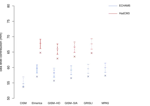
The additional cumulative sea level contribution due to the SMB-elevation feedback, under the A1B scenario and averaged over five ISM projections for ECHAM5 and three for HadCM3, is 4.3 % (best estimate; 95 % credibility interval 1.8–6.9 %) at 2100, and

15

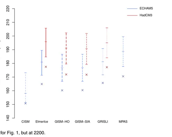
9.6 % (best estimate; 95 % credibility interval 3.6–16.0 %) at 2200 (Figs. 1 and 2; Ta-bles 1 and 2). We exclude GISM-SIA from all summary statistics presented because it is so similar in structure, and identical in set-up, to GISM-HO that it would eﬀ_ectively give double weighting to GISM. In all ISM predictions the elevation feedback is positive: the lower bounds of the 95 % CIs (the 2.5th percentile simulations) give larger sea level

20

contributions than the “no feedback” case. This is expected because the mean GrIS SMB becomes negative at around 2050 (Rae et al., 2012) and five of the six gradients (best estimate and 2.5th and 97.5th percentiles, for north and south) for negative SMB are positive (Edwards et al., 2013) thus adjusting the SMB in the same direction: more negative, giving greater sea level contribution. However, this was not guaranteed,

be-25

(13)

TCD

7, 675–708, 2013

Title Page

Tables Figures

◭ ◮

Back Close

Full Screen / Esc

Discussion

P

a

per

|

Dis

cussion

P

a

per

|

Discussion

P

a

per

|

Discussio

n

P

a

per

|

HadCM3-forced projection gives consistently higher sea level contributions than the ECHAM5-forced, because the HadCM3-forced MAR simulation projects greater melt-water runoﬀ_{(Rae et al., 2012).}

The Elmer/Ice and GRISLI total sea level contributions are virtually identical. This is a coincidence: the changes in ice discharge and SMB are diﬀ_{erent, but the di}ﬀ_erences 5

just compensate each other so that the sea level contributions are the same. The two models have similar initialisation procedures, but the diﬀ_{ering dynamic and SMB} re-sponses lead us to believe this is not the reason for the similar results. CISM seems to be an outlier in the ISM ensemble, particularly at 2200 (Fig. 2; Table 2), in both the no feedback result (low) and the magnitude of the feedback (small), though the latter may

10

be a result of the former. The GISM-SIA results are very similar to those of GISM-HO. This can be explained by the identical model setup and their similarity in response to perturbations; the only diﬀ_{erence between the two models is in the dynamic response,} which is a much smaller contribution than the SMB response (Fürst et al., 2013).

We can compare the projections with and without SMB-elevation feedback from the

15

two GCMs for the three ISMs that used both projections: Elmer/Ice, GISM-HO and GRISLI, from here on called the “starred” models (again, GISM-SIA is excluded here). Without elevation feedback, the mean GrIS sea level contributions at 2100 are 57 mm (ECHAM5) and 64 mm (HadCM3); with feedback, these increase by 3 mm (5 %). At 2200, the mean GrIS sea level contributions without feedback are 164 mm (ECHAM5)

20

and 176 mm (HadCM3); the feedback contributes an additional 16 mm (10 %) and 19 mm (11 %) respectively. The larger feedback adjustment at 2200 arises from the negative SMB forcing at the end of the first century which is sustained (by repetition of the decade 2090–2099 from the MAR simulation: Sect. 2.1) during the second century. The results show that not only does the contribution due to the feedback increase

25

(14)

TCD

7, 675–708, 2013

Title Page

Tables Figures

◭ ◮

Back Close

Full Screen / Esc

Discussion

P

a

per

|

Dis

cussion

P

a

per

|

Discussion

P

a

per

|

Discussio

n

P

a

per

|

between the two GCMs (averaged over the no feedback and three feedback estimates) for the three starred models is 7.8 mm; the mean spread of all five ISMs for ECHAM5 is 4.5 mm; and the mean 95 % CI (over all ISMs and GCMs) is 3.0 mm. But by 2200 (Fig. 2; Table 2), the relative importance has changed. The ISM spread and elevation feedback parameterisation uncertainty overtake the diﬀ_{erence between the two GCMs:} 5

the mean diﬀ_{erence between the two GCMs is 13.7 mm; the mean spread of ISMs for} ECHAM5 is 25.8 mm; and the mean 95 % CI (over all ISMs and GCMs) is 20.8 mm. In other words, the parameterisation and ISM uncertainties increase by a factor of seven and six respectively between 2100 and 2200, while the diﬀ_{erence between the two} GCMs barely doubles. The relative contributions to our uncertainty thus depend on the

10

timescale of interest.

This can be seen clearly in Fig. 3, which shows the fractional uncertainties as a func-tion of time with a 15 yr running mean applied. At the start of the projecfunc-tions, the ISM structural uncertainty explored (the range of five ISM best estimates divided by their mean, for the ECHAM5 projections) is a large fraction because the signal is small, but

15

the fraction decreases (the signal increases faster than the range) during the first half of the twentieth century. After this the fraction increases again (the range increases faster than the signal). The time-dependence of the GCM structural uncertainty explored (the diﬀ_{erence between ECHAM5 and HadCM3 results divided by their mean, averaged} over the best estimates for the three starred ISMs) appears at first glance to be

sim-20

ilar, but the underlying reason is diﬀ_{erent: it rapidly falls to a minimum when the two} GCMs projections happen to coincide for a short period (see also Rae et al., 2012). Af-ter a short increase due to the GCMs diverging again, the fractional uncertainty slowly falls because the signal increases faster than the range. The fractional uncertainty due to the parameterisation (95 % CI divided by the best estimate, averaged over all ISMs

25

(15)

TCD

7, 675–708, 2013

Title Page

Tables Figures

◭ ◮

Back Close

Full Screen / Esc

Discussion

P

a

per

|

Dis

cussion

P

a

per

|

Discussion

P

a

per

|

Discussio

n

P

a

per

|

The GISM-SIA PPE gives the entire sea level probability distribution (Fig. 4) rather than just the 95 % CIs. We can inspect any other interval, such as the 90 % CI (177.3– 194.7 mm) or 50 % CI (182.3–190.6 mm). We can also test whether the projected distri-bution of sea level contridistri-butions is symmetric about the best estimate (186.1 mm). The 95 % CI, is symmetric (±10.4 mm), and the 90 % CI nearly so (−8.8 mm,+_{8.6 mm), but} 5

the 50 % interval (−3.8 mm, +_{3.5 mm) indicates the probability density leans slightly} towards the higher sea level contributions.

The unimodal and (broadly) symmetric shape of the PPE sea level distribution likely reflects the unimodal and (in most cases) symmetric shapes of the four posterior prob-ability distributions of the gradient values (Edwards et al., 2013), combined with the

lin-10

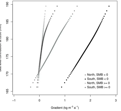
ear model of adjustment. Figure 5 shows the dependence of the sea level contribution on the gradient sets. This cannot show which of the four gradients is most important, because they are varied simultaneously. But it illustrates the following: the relationship between sea level contribution and gradient set is mostly linear; the two gradients for below the ELA are the most uncertain (largest range in kg m−3a−1); and the

gradi-15

ent for above the ELA, south of 77◦N, has the least symmetric probability distribution (equally-spaced samples in probability become increasingly far apart in kg m−3a−1).

4 Discussion

4.1 Elevation feedback

These results are the first application of an SMB-elevation parameterisation to RCM

20

projections. Our method allows ISMs to be forced with the more physically realistic simulations of SMB from RCMs, rather than their own simpler PDD schemes, while incorporating the elevation feedback and exploring model uncertainties. Another use would be to correct low resolution MAR simulations onto a high resolution digital ele-vation map; the diﬀ_{erence in elevation between the two topographies is analogous to} 25

(16)

TCD

7, 675–708, 2013

Title Page

Tables Figures

◭ ◮

Back Close

Full Screen / Esc

Discussion

P

a

per

|

Dis

cussion

P

a

per

|

Discussion

P

a

per

|

Discussio

n

P

a

per

|

of MAR SMB simulations, which would be useful not only for forcing ISMs but also comparing with observations. The advantages of our parameterisation method over previous studies are described in the companion paper (Edwards et al., 2013).

It is important to try and quantify the magnitude of the SMB-elevation feedback rel-ative to projections without it (such as Rae et al., 2012). Despite the negrel-ative gradient

5

values we present in Edwards et al. (2013), the lower bounds of our 95 % CIs with feed-back are always greater than the projections without feedfeed-back. But our results indicate that the additional contribution is relatively small (best estimates 5 % at 2100, 10–11 % at 2200), so century-long simulations with coupled RCM-ISM models may not be jus-tified for the additional computational expense and technical diﬃ_{culty of coupling. On} 10

the other hand, A1B is a medium-high emission scenario. When forced by the GCM MIROC5 under the high-end Representative Concentration Pathway RCP8.5 (Moss et al., 2010), MAR projections using perturbed ice sheet topographies consistent with SMB changes show an additional mass loss of 5–15 % over just one century (Fettweis et al., 2012). However, this estimate is with respect to projected SMB changes, while

15

our results are evaluated with respect to the total mass change (SMB plus dynamic changes). In addition, the SMB-elevation feedback estimate from Fettweis et al. (2012) is made by perturbing the MAR ice sheet topography with corrections equivalent to the cumulative projected SMB changes over 2000–2079 without coupling MAR to an ice sheet model. In reality the ice sheet dynamics should partly compensate the

sur-20

face height decreases from the melt increase in the ablation zone, by redistributing the additional mass gained at the top of the ice sheet, so the Fettweis et al. (2012) esti-mates likely overestimate this contribution. Only a coupled RCM-ISM would allow full simulation of the SMB-elevation feedback.

Previously some have suggested that PDD descriptions of ice sheet response are too

25

(17)

TCD

7, 675–708, 2013

Title Page

Tables Figures

◭ ◮

Back Close

Full Screen / Esc

Discussion

P

a

per

|

Dis

cussion

P

a

per

|

Discussion

P

a

per

|

Discussio

n

P

a

per

|

parameterisation with the GISM PDD scheme, using the same ice sheet extent and RCM. Helsen et al. (2011) also compare their parameterisation of the RACMO2/GR SMB-elevation feedback with PDD results. In both cases, the PDD schemes predict a smaller sea level contribution in a warmer climate than the RCMs: for example, Goelzer et al. (2013) find the PDD model gives a 14–33 % lower sea level contribution

5

than MAR. There are many diﬀ_{erences between physically-based energy balance RCM} schemes and empirical PDD schemes, including the presence of albedo feedback in the RCMs, higher spatial resolution in the PDD schemes, and diﬀ_{erent treatment of} re-freezing (Goelzer et al., 2013). Our parameterisation of the MAR SMB-elevation feed-back as four probability distributions is a more complex representation of the feedfeed-back

10

than PDD schemes, which use a fixed temperature lapse rate: it incorporates the pre-cipitation aspect, and the variation of the feedback with climate, topography, and region. However, the response of SMB to a modified topography is complex and nonlinear. Even with full inclusion of uncertainties, a gradient-based (i.e. linear) parameterisation cannot fully represent the SMB changes that would be modelled by a fully coupled

15

RCM-ISM.

4.2 Modelling uncertainties

Our method is novel because we propagate three types of model uncertainty – GCM structural uncertainty, ISM structural uncertainty, and elevation feedback parameteri-sation uncertainty – along the causal chain from SRES scenario to sea level within

20

a coherent experimental design and statistical framework. In particular, parameter un-certainty is estimated with a probabilistic method, which gives well-defined credibility intervals (CIs) rather than simple sensitivity tests; all ISMs use the same parameterisa-tion and parameter sampling, and are forced with the same GCMs and RCM, enabling comparisons across ISMs; and MAR is forced with two GCM forcings under the same

25

(18)

TCD

7, 675–708, 2013

Title Page

Tables Figures

◭ ◮

Back Close

Full Screen / Esc

Discussion

P

a

per

|

Dis

cussion

P

a

per

|

Discussion

P

a

per

|

Discussio

n

P

a

per

|

importance of a range of parametric and structural uncertainties and how these vary with time. We refer to Fettweis et al. (2012) for a discussion of the eﬀ_{ects of changing} the MAR tundra/ice mask and ice sheet topography, and using a range of GCMs for forcing, on simulations of current climate and projections of future climate change.

Parametric uncertainties result in a unimodal and fairly symmetric probability

distri-5

bution for sea level contribution (Fig. 4), because of the linear SMB adjustment and the sampling from unimodal and (in most cases) symmetric probability distributions for the gradients (Edwards et al., 2013). If the gradient distributions derived from MAR were strongly asymmetric or multimodal, or the SMB adjustment nonlinear, the sea level distribution might be a diﬀ_{erent shape. Here is the real value of Bayesian estimation} 10

of parameters (Edwards et al., 2013) and sampling these uncertainties with perturbed parameter ensembles, because such things are generally not known in advance. The slight asymmetry in the sea level probability distribution described in the previous sec-tion might become more pronounced for timescales longer than two centuries.

If substantial computational resources and time are available, a more thorough

ex-15

ploration of parametric uncertainty would perturb other parameters of the ISMs and parameters of the climate models. Climate model PPEs are used extensively by Mur-phy et al. (2009). Two ISM PPEs are presented by Stone et al. (2010) and Applegate et al. (2011), who vary multiple parameters simultaneously in order to explore their in-teractions. For example, surface lowering driven by parameterised dynamic processes

20

(such as basal lubrication: Shannon et al., 2013) could interact diﬀ_{erently with the} ele-vation feedback depending on the values of the relevant parameters. Performing multi-ple parameter perturbations might aﬀ_{ect the shape of the distribution of projected sea} level contributions.

Structural uncertainties are much more challenging to assess, because there is no

25

(19)

TCD

7, 675–708, 2013

Title Page

Tables Figures

◭ ◮

Back Close

Full Screen / Esc

Discussion

P

a

per

|

Dis

cussion

P

a

per

|

Discussion

P

a

per

|

Discussio

n

P

a

per

|

extent to which an ensemble of models represents our uncertainty about the system they simulate. Nonetheless, it is clearly better to sample from this space, to explore it partially, than to ignore it.

Here the structural uncertainty explored most is in the ISMs (an ensemble of five). Structural diﬀ_{erences in ice sheet modelling includes representation of the Stokes} 5

equations, numerical methods, grid resolution, initialisation procedures, and drift cor-rection. Goelzer et al. (2013) compare GrIS sea level projections for diﬀ_{erent model} formulations. We explore some GCM structural uncertainty by using two GCMs. We emphasise that we do not claim to quantify ISM and GCM structural uncertainties, only to sample from them. Our multi-model ensembles are small, and models have common

10

components and errors that are likely to reduce the ensemble range relative to our ac-tual uncertainty about the climate and GrIS. However, using multi-model ensembles is a necessary first step along that path.

We do not explore RCM structural uncertainty. An ensemble of RCMs would require a new parameterisation of the SMB-elevation feedback for each. We do incorporate

15

uncertainty in the structure of our parameterisation of MAR by including a discrepancy variance term when estimating the gradients (Edwards et al., 2013). We emphasis that this discrepancy variance refers to our parameterisation of the MAR elevation feed-back, not the MAR simulation of the feedback in the real world. The latter is the RCM structural uncertainty. We could sample from this with multiple RCMs, but quantifying

20

it is very challenging due to their computational expense; such estimates are relatively rare (e.g. Sexton and Murphy, 2011).

We note that a small spread in model results does not correspond to certainty about the future: for example, models may not be independent (e.g. share code), or might co-incidentally give similar results for diﬀ_{erent reasons (such as Elmer/Ice and GRISLI). It} 25

(20)

TCD

7, 675–708, 2013

Title Page

Tables Figures

◭ ◮

Back Close

Full Screen / Esc

Discussion

P

a

per

|

Dis

cussion

P

a

per

|

Discussion

P

a

per

|

Discussio

n

P

a

per

|

Our quantification of the relative magnitude of modelling uncertainties through time (Fig. 3) is therefore specific to our particular choices and opportunities: the RCM, GCMs and ISMs; the emissions scenario; our method of extending the scenario from 2100 to 2199; and (trivially) our chosen CI width. If we used a scenario in which the SMB projections were more negative than for A1B, such as RCP8.5, or less negative,

5

such as E1 (Rae et al., 2012), the elevation feedback would be correspondingly larger or smaller and so would the uncertainty. Similarly, if we were to use 200 yr GCM and RCM simulations, i.e. drive MAR with GCM simulations that were forced in the second century with the A1B scenario at 2100, rather than repeating the decade 2090–2099 from the MAR simulations ten times, the SMB forcing would likely continue to decrease

10

rather than remain fixed. This would lead to a more rapid increase in the sea level projections with elevation feedback. The ISM fractional uncertainty might then not in-crease in the second century, or not as much (Fig. 3); this would depend on the rel-ative responses of the ISMs. The GCM range might increase more quickly than the mean, giving a time-dependent fractional uncertainty that is more similar in shape to

15

the ISM fractional uncertainty (Fig. 3). Such choices are unavoidable given the sub-stantial computational expense of a three stage model chain in which two stages are climate models. Nevertheless, this work begins the process of determining where to focus computational resources and model development for diﬀ_{erent decision-making} timescales.

20

5 Summary

We present the first application of a parameterisation of the GrIS SMB-elevation feed-back to projections of future climate change. This is currently the only practicable method for making projections for the GrIS contribution to sea level that can incorporate physical modelling of ice flow, SMB processes, and the SMB-elevation feedback while

25

(21)

TCD

7, 675–708, 2013

Title Page

Tables Figures

◭ ◮

Back Close

Full Screen / Esc

Discussion

P

a

per

|

Dis

cussion

P

a

per

|

Discussion

P

a

per

|

Discussio

n

P

a

per

|

and statistical framework. Projections are made for the SRES A1B emissions scenario with the MAR RCM, ECHAM5 and HadCM3 GCMs, and five ISMs. The experimen-tal design allows us to estimate the relative importance of these model uncertainties, and how they vary over time, for the GrIS contribution to sea level over the next two centuries.

5

The additional sea level contribution due to the SMB-elevation feedback, averaged over five ISM projections for ECHAM5 and three for HadCM3 is 4.4 % (best estimate; 95 % credibility interval 1.8–6.9 %) at 2100, and 9.6 % (best estimate; 95 % credibility interval 3.6–16.0 %) at 2200. In all results, the lower bounds of our 95 % credibility intervals for sea level contributions with the SMB-elevation feedback are larger than for

10

the “no feedback” case.

The relative contributions to uncertainty vary with time. In 2100, the GCM diﬀ_erences are larger than the ISM range and the parameterisation uncertainty, but by 2200, the ISM and parameterisation uncertainties are greater. This work indicates that the areas where future research should be directed – such as understanding climate or ice sheet

15

model diﬀ_{erences, or performing perturbed parameter ensembles – depends on the} time scale of interest. For suﬃ_{ciently large ensemble sizes, this method can be used} to give an indication where future sea level research should be directed.

Acknowledgements. This work was supported by funding from the ice2sea programme from the European Union 7th Framework Programme, grant number 226375. Ice2sea contribution 20

(22)

TCD

7, 675–708, 2013

Title Page

Tables Figures

◭ ◮

Back Close

Full Screen / Esc

Discussion

P

a

per

|

Dis

cussion

P

a

per

|

Discussion

P

a

per

|

Discussio

n

P

a

per

|

References

Applegate, P. J., Kirchner, N., Stone, E. J., Keller, K., and Greve, R.: An assessment of key model parametric uncertainties in projections of Greenland Ice Sheet behavior, The Cryosphere, 6, 589–606, doi:10.5194/tc-6-589-2012, 2012. 692

Bamber, J. L., Hardy, R. J., and Joughin, I.: An analysis of balance velocities over the Greenland 5

ice sheet and comparison with synthetic aperture radar interferometry, J. Glaciol., 46, 67–74, 2000. 682

Bindschadler, R. A., Nowicki, S., Abe-Ouchi, A., Aschwanden, A., Choi, H., Fastook, J., Granzow, G., Greve, R., Gutowski, G., Herzfeld, U., Jackson, C., Johnson, J., Khroulev, C., Levermann, A., Lipscomb, W. H., Martin, M. A., Morlighem, M., Parizek, B. R., Pollard, D., 10

Price, S. F., Ren, D., Saito, F., Sato, T., Seddik, H., Seroussi, H., Takahashi, K., Walker, R., and Wang, W. L.: Ice-sheet model sensitivities to environmental forcing and their use in pro-jecting future sealevel (the SeaRISE project), J. Glaciol., accepted, 2013. 679

Bueler, E. and Brown, J.: Shallow shelf approximation as a “sliding law” in a thermomechanically coupled ice sheet model, J. Geophys. Res., 114, F03008, doi:10.1029/2008JF001179, 2009. 15

681, 682

Dee, D. P., Uppala, S. M., Simmons, A. J., Berrisford, P., Poli, P., Kobayashi, S., Andrae, U., Balmaseda, M. A., Balsamo, G., Bauer, P., Bechtold, P., Beljaars, A. C. M., van de Berg, L., Bidlot, J., Bormann, N., Delsol, C., Dragani, R., Fuentes, M., Geer, A. J., Haimberger, L., Healy, S. B., Hersbach, H., Hólm, E. V., Isaksen, L., K ˙allberg, P., Köhler, M., Matricardi, M., 20

McNally, A. P., Monge-Sanz, B. M., Morcrette, J.-J., Park, B.-K., Peubey, C., de Rosnay, P., Tavolato, C., Thépaut, J.-N., and Vitart, F.: The ERA-Interim reanalysis: configuration and performance of the data assimilation system, Q. J. Roy. Meteor. Soc., 137, 553–597, 2011. 680

Edwards, T. L., Fettweis, X., Gagliardini, O., Gillet-Chaulet, F., Goelzer, H., Gregory, J. M., 25

Hoﬀ_{man, M., Huybrechts, P., Payne, A. J., Perego, M., Price, S., Ritz, C., and Quiquet, A.:} Eﬀ_{ect of uncertainty in surface mass balance–elevation feedback on projections of the future} sea level contribution of the Greenland ice sheet – Part 1: Parameterisation, The Cryosphere Discuss., 7, 635–674, doi:doi:10.5194/tcd-7-635-2013, 2013. 677, 678, 679, 680, 685, 686, 689, 690, 692, 693

30

(23)

TCD

7, 675–708, 2013

Title Page

Tables Figures

◭ ◮

Back Close

Full Screen / Esc

Discussion

P

a

per

|

Dis

cussion

P

a

per

|

Discussion

P

a

per

|

Discussio

n

P

a

per

|

sheet revealed by high-resolution climate modeling, Geophys. Res. Lett., 36, L12501, doi:10.1029/2009GL038110, 2009. 678

Evans, K. J., Salinger, A. G., Worley, P. H., Price, S. F., Lipscomb, W. H., Nicols, J. A., White III, J. B., Perego, M., Vertenstein, M., Edwards, J., and Lemieux, J. F.: A modern solver interface to manage solution algorithms in the Community Earth System Model, Int. J. High 5

Perform. C, 26, 54–62, 2012. 682

Fettweis, X.: Reconstruction of the 1979–2006 Greenland ice sheet surface mass balance us-ing the regional climate model MAR, The Cryosphere, 1, 21–40, doi:10.5194/tc-1-21-2007, 2007. 678, 680

Fettweis, X., Franco, B., Tedesco, M., van Angelen, J. H., Lenaerts, J. T. M., 10

van den Broeke, M. R., and Gallée, H.: Estimating Greenland ice sheet surface mass bal-ance contribution to future sea level rise using the regional atmospheric climate model MAR, The Cryosphere Discuss., 6, 3101–3147, doi:10.5194/tcd-6-3101-2012, 2012. 679, 684, 690, 692

Franco, B., Fettweis, X., and Erpicum, M.: Future projections of the Greenland ice sheet en-15

ergy balance driving the surface melt, The Cryosphere, 7, 1–18, doi:10.5194/tc-7-1-2013, 2013. 680

Fürst, J. J., Rybak, O., Goelzer, H., De Smedt, B., de Groen, P., and Huybrechts, P.: Improved convergence and stability properties in a three-dimensional higher-order ice sheet model, Geosci. Model Dev., 4, 1133–1149, doi:10.5194/gmd-4-1133-2011, 2011. 681

20

Fürst, J. J., Goelzer, H., and Huybrechts, P.: Eﬀ_{ect of higher-order stress gradients on} the centennial mass evolution of the Greenland ice sheet, The Cryosphere, 7, 183–199, doi:10.5194/tc-7-183-2013, 2013. 681, 687

Gillet-Chaulet, F., Gagliardini, O., Seddik, H., Nodet, M., Durand, G., Ritz, C., Zwinger, T., Greve, R., and Vaughan, D. G.: Greenland ice sheet contribution to sea-level rise from a new-25

generation ice-sheet model, The Cryosphere, 6, 1561–1576, doi:10.5194/tc-6-1561-2012, 2012. 682

Goelzer, H., Huybrechts, P., Fürst, J. J., Andersen, M. L., Edwards, T. L., Fettweis, X., Nick, F. M., Payne, A. J., and Shannon, S. R.: Sensitivity of Greenland ice sheet projections to model formulations, J. Glaciol., in review, 2013. 682, 690, 691, 693

30

(24)

TCD

7, 675–708, 2013

Title Page

Tables Figures

◭ ◮

Back Close

Full Screen / Esc

Discussion

P

a

per

|

Dis

cussion

P

a

per

|

Discussion

P

a

per

|

Discussio

n

P

a

per

|

of the Hadley Centre coupled model without flux adjustments, Clim. Dynam., 16, 147–168, 2000. 680

Greve, R.: A continuum-mechanical formulation for shallow polythermal ice sheets, Philos. T. Roy. Soc. A, 355, 217–242, 1997. 682

Griggs, J. A., Bamber, J. L., Hurkmans, R. T. W. L., Dowdesewell, J. A., Gogineni, S. P., 5

Howat, I., Mouginot, J., Paden, J., Palmer, S., Rignot, E., and Steinhage, D.: A new bed elevation dataset for Greenland, The Cryosphere Discuss., 6, 4829–4860, doi:10.5194/tcd-6-4829-2012, 2012. 682, 684

Hanna, E., Huybrechts, P., Cappelen, J., Steff_{en, K., Bales, R. C., Burgess, E., McConnell, J. R.,} Peder Steff_{ensen, J., van den Broeke, M., Wake, L., Bigg, G., Gri}ffi_{ths, M., and Deniz} 10

Savas, D.: Greenland Ice Sheet surface mass balance 1870 to 2010 based on Twentieth Century Reanalysis, and links with global climate forcing, J. Geophys. Res., 116, D24121, doi:10.1029/2011JD016387, 2011. 683, 690

Helsen, M. M., van de Wal, R. S. W., van den Broeke, M. R., van de Berg, W. J., and Oerle-mans, J.: Coupling of climate models and ice sheet models by surface mass balance gradi-15

ents: application to the Greenland Ice Sheet, The Cryosphere, 6, 255–272, doi:10.5194/tc-6-255-2012, 2012. 690, 691

Huybrechts, P. and de Wolde, J.: The dynamic response of the Greenland and Antarctic ice sheets to multiple-century climatic warming, J. Climate, 12, 2169–2188, 1999. 681

Janssens, I. and Huybrechts, P.: The treatment of meltwater retention in mass-balance param-20

eterizations of the Greenland ice sheet, Ann. Glaciol., 31, 133–140, 2000. 678

Joughin, I., Smith, B. E., Howat, I. M., Scambos, T., and Moon, T.: Greenland flow variability from ice-sheet-wide velocity mapping, J. Glaciol., 56, 415–430, 2010. 682

Lemieux, J. F., Price, S. F., Evans, K. J., Knoll, D., Salinger, A. G., Holland, D. M., and Payne, A. J.: Implementation of the Jacobian-free Newton–Krylov method for solving the 25

first-order ice sheet momentum balance, J. Comput. Phys., 230, 6531–6545, 2011. 682 Morlighem, M., Rignot, E., Seroussi, H., Larour, E., Dhia, H. B., and Aubry, D.:

Spa-tial patterns of basal drag inferred using control methods from a full-Stokes and sim-pler models for Pine Island Glacier, West Antarctica, Geophys. Res. Lett., 37, L14502, doi:10.1029/2010GL043853, 2010. 683

30

(25)

gen-TCD

7, 675–708, 2013

Title Page

Tables Figures

◭ ◮

Back Close

Full Screen / Esc

Discussion

P

a

per

|

Dis

cussion

P

a

per

|

Discussion

P

a

per

|

Discussio

n

P

a

per

|

eration of scenarios for climate change research and assessment, Nature, 463, 747–756, 2010. 690

Murphy, J. M., Sexton, D. M. H., Jenkins, G. J., Booth, B. B. B., Brown, C. C., Clark, R. T., Collins, M., Harris, G. R., Kendon, E. J., Betts, R. A., Brown, S. J., Humphrey, K. A., Mc-Carthy, M. P., McDonald, R. E., Stephens, A., Wallace, C., Warren, R., Wilby, R., and 5

Wood, R. A.: Climate change projections, in: UK Climate Projections, no. 2, Met Oﬃ_{ce Hadley} Centre, Exeter, UK, 1–194, 2009. 692

Nakić_enović_{, N., Alcamo, J., Davis, G., and de Vries, B.: Special report on emissions scenarios:} a special report of Working Group III of the Intergovernmental Panel on Climate Change, Intergovernmental Panel on Climate Change, 2000. 679, 681

10

Pattyn, F.: A new three-dimensional higher-order thermomechanical ice sheet model: basic sensitivity, ice stream development, and ice flow across subglacial lakes, J. Geophys. Res., 108, 2382, doi:10.1029/2002JB002329, 2003. 681

Pattyn, F., Schoof, C., Perichon, L., Hindmarsh, R. C. A., Bueler, E., de Fleurian, B., Durand, G., Gagliardini, O., Gladstone, R., Goldberg, D., Gudmundsson, G. H., Huybrechts, P., Lee, V., 15

Nick, F. M., Payne, A. J., Pollard, D., Rybak, O., Saito, F., and Vieli, A.: Results of the Marine Ice Sheet Model Intercomparison Project, MISMIP, The Cryosphere, 6, 573–588, doi:10.5194/tc-6-573-2012, 2012. 679

Perego, M., Gunzburger, M., and Burkardt, J.: Parallel finite element implementation for higher-order ice-sheet models, J. Glaciol., 58, 76–88, 2012. 682

20

Price, S. F., Payne, A. J., Howat, I. M., and Smith, B. E.: Committed sea-level rise for the next century from Greenland ice sheet dynamics during the past decade, P. Natl. Acad. Sci. USA, 108, 8978–8983, 2011. 682

Quiquet, A., Punge, H. J., Ritz, C., Fettweis, X., Gallée, H., Kageyama, M., Krinner, G., Salas y Mélia, D., and Sjolte, J.: Sensitivity of a Greenland ice sheet model to atmospheric 25

forcing fields, The Cryosphere, 6, 999–1018, doi:10.5194/tc-6-999-2012, 2012. 682 Rastner, P., Bolch, T., Mölg, N., Machguth, H., and Paul, F.: The first complete glacier inventory

for the whole of Greenland, The Cryosphere Discuss., 6, 2399–2436, doi:10.5194/tcd-6-2399-2012, 2012. 683

Ringler, T., Ju, L., and Gunzburger, M.: A multiresolution method for climate system modeling: 30

(26)

TCD

7, 675–708, 2013

Title Page

Tables Figures

◭ ◮

Back Close

Full Screen / Esc

Discussion

P

a

per

|

Dis

cussion

P

a

per

|

Discussion

P

a

per

|

Discussio

n

P

a

per

|

Ritz, C., Rommeleare, V., and Dumas, C.: Modeling the evolution of Antarctic ice sheet over the last 420 000 yr: Implications for altitude changes in the Vostok region, J. Geophys. Res., 106, 31943–31964, 2001. 682

Rutt, I., Hagdorn, M., Hulton, N., and Payne, A.: The “Glimmer” community ice sheet model, J. Geophys. Res., 114, F02004, doi:10.1029/2008JF001015, 2009. 682

5

Rae, J. G. L., Aðalgeirsdóttir, G., Edwards, T. L., Fettweis, X., Gregory, J. M., Hewitt, H. T., Lowe, J. A., Lucas-Picher, P., Mottram, R. H., Payne, A. J., Ridley, J. K., Shannon, S. R., van de Berg, W. J., van de Wal, R. S. W., and van den Broeke, M. R.: Greenland ice sheet surface mass balance: evaluating simulations and making projections with regional climate models, The Cryosphere, 6, 1275–1294, doi:10.5194/tc-6-1275-2012, 2012. 679, 684, 686, 10

687, 688, 690, 694

Roeckner, E., Bäuml, G., Bonaventura, L., Brokopf, R., Esch, M., Giorgetta, M., Hagemann, S., Kirchner, I., Kornblueh, L., Manzini, E., Rhodin, A., Schlese, U., Schulzweida, U., and Tomp-kins, A.: The atmospheric general circulation model ECHAM 5. Part I: Model description, Max-Planck-Institut für Meteorologie, Hamburg, Germany, 126 pp., 2003. 680

15

Sexton, D. and Murphy, J.: Multivariate probabilistic projections using imperfect climate models. Part II: Robustness of methodological choices and consequences for climate sensitivity, Clim. Dynam., 38, 2543–2558, 2011. 679, 693

Sexton D. M. H., Murphy, J., Collins, M., and Webb, M.: Multivariate probabilistic projections using imperfect climate models. Part I: Outline of methodology, Clim. Dynam., 38, 2513– 20

2542, 2011. 679

Shannon, S. R., Payne, A. J., Bartholomew, I. D., van den Broeke, M. R., Edwards, T. L., Fet-tweis, X., Gagliardini, O., Gillet-Chaulet, F., Goelzer, H., Hoﬀ_{man, M., Huybrechts, P., Mair, D.,} Nienow, P., Perego, M., Price, S. F., Smeets, C. J. P. P., Sole, A. J., van de Wal, R. S. W., and Zwinger, T.: Enhanced basal lubrication and the contribution of the Greenland ice sheet to 25

future sea level rise, P. Natl. Acad. Sci. USA, in review, 2013. 691, 692

Shapiro, N. M. and Ritzwoller, M. H.: Inferring surface heat flux distributions guided by a global seismic model: particular application to Antarctica, Earth Planet. Sc. Lett., 223, 213–224, 2004. 682

Stone, E. J., Lunt, D. J., Rutt, I. C., and Hanna, E.: Investigating the sensitivity of numerical 30

(27)

TCD

7, 675–708, 2013

Title Page

Tables Figures

◭ ◮

Back Close

Full Screen / Esc

Discussion

P

a

per

|

Dis

cussion

P

a

per

|

Discussion

P

a

per

|

Discussio

n

P

a

per

|

Uppala, S. M., Køallberg, P. W., Simmons, A. J., Andrae, U., Da Costa Bechtold, V., Fiorino, M., Gibson, J. K., Haseler, J., Hernandez, A., Kelly, G. A., Li, X., Onogi, K., Saarinen, S., Sokka, N., Allan, R. P., Andersson, E., Arpe, K., Balmaseda, Bel-jaars, A. C. M., Van De Berg, L., Bidlot, J., Bormann, N., Caires, S., Chevallier, F., Dethof, A., Dragosavac, M., Fisher, M., Fuentes, M., Hagemann, S., Hólm, E., Hoskins, B. J., Isaksen L., 5

Janssen, P. A. E. M., Jenne, R., Mcnally, A. P., Mahfouf, J.-F., Morcrette, J.-J., Rayner, N. A., Saunders, R. W., Simon, P., Sterl, A., Trenberth, K. E., Untch, A., Vasiljevic, D., Viterbo, P., Woollen, J.: The ERA-40 re-analysis, Q. J. Roy. Meteor. Soc., 131, 2961–3012, 2005. 683 van de Berg, W. J., van den Broeke, M., Ettema, J., van Meijgaard, E., and Kaspar, F.:

Signifi-cant contribution of insolation to Eemian melting of the Greenland ice sheet, Nat. Geosci., 4, 10

679–683, 2011. 690

van de Wal, R. S. W.: Mass-balance modelling of the Greenland ice sheet: a comparison of an energy-balance and a degree-day model, Ann. Glaciol., 23, 36–45, 1996. 690

Vernon, C. L., Bamber, J. L., Box, J. E., van den Broeke, M. R., Fettweis, X., Hanna, E., and Huybrechts, P.: Surface mass balance model intercomparison for the Greenland ice sheet, 15

(28)

TCD

7, 675–708, 2013

Title Page

Tables Figures

◭ ◮

Back Close

Full Screen / Esc

Discussion

P

a

per

|

Dis

cussion

P

a

per

|

Discussion

P

a

per

|

Discussio

n

P

a

per

|

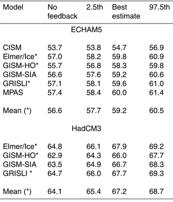
Table 1.Projected sea level contribution (mm) at 2100 for the ECHAM5 (top) and HadCM3

(bottom) A1B projections: no feedback, 2.5th percentile, best, and 97.5th percentile estimates.

Model No 2.5th Best 97.5th feedback estimate

ECHAM5

CISM 53.7 53.8 54.7 56.9 Elmer/Ice* 57.0 58.2 59.8 60.9 GISM-HO* 55.7 56.8 58.3 59.8 GISM-SIA 56.6 57.6 59.2 60.6 GRISLI* 57.1 58.1 59.6 61.0 MPAS 57.4 58.4 60.0 61.4

Mean (*) 56.6 57.7 59.2 60.5

HadCM3

Elmer/Ice* 64.8 66.1 67.9 69.2 GISM-HO* 62.9 64.3 66.0 67.7 GISM-SIA 63.5 64.9 66.7 68.3 GRISLI * 64.7 66.0 67.7 69.3

(29)

TCD

7, 675–708, 2013

Title Page

Tables Figures

◭ ◮

Back Close

Full Screen / Esc

Discussion

P

a

per

|

Dis

cussion

P

a

per

|

Discussion

P

a

per

|

Discussio

n

P

a

per

|

Table 2.As for Table 1, but at 2200.

Model No 2.5th Best 97.5th feedback estimate

ECHAM5

CISM 150.8 151.3 158.1 173.1 Elmer/Ice* 164.9 171.3 181.0 189.5 GISM-HO* 160.3 166.9 176.7 186.6 GISM-SIA 160.4 166.9 176.8 186.6 GRISLI* 165.7 171.6 181.2 190.8 MPAS 170.5 177.7 188.7 199.6

Mean (*) 163.6 169.9 179.6 189.0

HadCM3

Elmer/Ice* 177.5 184.7 195.8 205.7 GISM-HO* 171.9 179.6 191.1 202.3 GISM-SIA 171.7 179.3 190.7 201.9 GRISLI* 177.2 184.1 195.0 206.0

(30)

TCD

7, 675–708, 2013

Title Page

Tables Figures

◭ ◮

Back Close

Full Screen / Esc

Discussion

P

a

per

|

Dis

cussion

P

a

per

|

Discussion

P

a

per

|

Discussio

n

P

a

per

|

Sea le

vel contr

ib

ution (mm)

50

55

60

65

70

75

80

CISM ElmerIce GISM−HO GISM−SIA GRISLI MPAS

ECHAM5

HadCM3

Fig. 1.Projected cumulative GrIS sea level contributions for the ECHAM5 and HadCM3 A1B

Effect of uncertainty in surface mass balance elevation feedback on projections of the future sea level contribution of the Greenland ice sheet &ndash; Part 2: Projections

TCD

E

ff

ect of uncertainty in surface mass

balance elevation feedback on projections

of the future sea level contribution of the

Greenland ice sheet – Part 2: Projections

TCD

TCD

TCD

TCD

TCD

TCD

TCD

TCD

TCD

TCD

TCD

TCD

TCD

TCD

TCD

TCD

TCD

TCD

TCD

TCD

TCD

TCD

TCD

gen-TCD

TCD

TCD

TCD

TCD

TCD

Effect of uncertainty in surface mass balance elevation feedback on projections of the future sea level contribution of the Greenland ice sheet – Part 2: Projections

_ff