www.biogeosciences.net/8/1881/2011/ doi:10.5194/bg-8-1881-2011
© Author(s) 2011. CC Attribution 3.0 License.
Biogeosciences
A coupled physical-biological model of the Northern Gulf of Mexico
shelf: model description, validation and analysis of phytoplankton
variability
K. Fennel1, R. Hetland2, Y. Feng2, and S. DiMarco2
1Department of Oceanography, Dalhousie University, Halifax, Nova Scotia, Canada 2Department of Oceanography, Texas A&M University, College Station, Texas, USA
Received: 16 December 2010 – Published in Biogeosciences Discuss.: 7 January 2011 Revised: 7 June 2011 – Accepted: 30 June 2011 – Published: 13 July 2011
Abstract. The Texas-Louisiana shelf in the Northern Gulf of Mexico receives large inputs of nutrients and freshwater from the Mississippi/Atchafalaya River system. The nutri-ents stimulate high rates of primary production in the river plume, which contributes to the development of a large and recurring hypoxic area in summer, but the mechanistic links between hypoxia and river discharge of freshwater and nu-trients are complex as the accumulation and vertical export of organic matter, the establishment and maintenance of ver-tical stratification, and the microbial degradation of organic matter are controlled by a non-linear interplay of factors. Un-raveling these interactions will have to rely on a combination of observations and models. Here we present results from a realistic, 3-dimensional, physical-biological model with fo-cus on a quantification of nutrient-stimulated phytoplank-ton growth, its variability and the fate of this organic mat-ter. We demonstrate that the model realistically reproduces many features of observed nitrate and phytoplankton dynam-ics including observed property distributions and rates. We then contrast the environmental factors and phytoplankton source and sink terms characteristic of three model subre-gions that represent an ecological gradient from eutrophic to oligotrophic conditions. We analyze specifically the reasons behind the counterintuitive observation that primary produc-tion in the light-limited plume region near the Mississippi River delta is positively correlated with river nutrient input, and find that, while primary production and phytoplankton
Correspondence to: K. Fennel
biomass are positively correlated with nutrient load, phyto-plankton growth rate is not. This suggests that accumulation of biomass in this region is not primarily controlled bottom up by nutrient-stimulation, but top down by systematic dif-ferences in the loss processes.
1 Introduction
The Texas-Louisiana shelf in the Northern Gulf of Mexico is dominated by large seasonal inputs of freshwater and inor-ganic and orinor-ganic nutrients from the Mississippi/Atchafalaya River system. The Mississippi River is one of the world’s major rivers; it has the third largest drainage basin, is the fifth largest in terms of freshwater discharge and seventh largest in terms of sediment discharge compared with other world rivers (Milliman and Meade, 1983). The Mississippi River drains 41 % of the contiguous USA, including agricultural land in Southern Minnesota, Iowa, Illinois and Ohio, which contributes about one third of the nitrogen loading of the river (Goolsby et al., 2000). The greatest nitrogen loading comes from tile-drained fields in the cornbelt of the midwest (David et al., 2010). The mean annual nitrogen load to the Gulf of Mexico of 1.5 Mt yr−1consists of approximately 61 % ni-trate, 37 % organic nitrogen and 2 % ammonium (1980–1996 mean), and the nitrate load has approximately tripled from 1970 to the late 90ies (Goolsby et al., 2000).
classic concept of coastal eutrophication leading to hypoxia and often applied to this region is as follows. Inorganic nutri-ents from the Mississippi fuel high rates of primary produc-tion as the discharged river water spreads in buoyant plumes over the shelf, and, as this organic matter sinks below the pycnocline and is respired microbially, oxygen consumption exceeds supply in bottom waters and hypoxia develops. The existence of statistically significant relationships between the annual Mississippi River nitrogen load and the spatial extent of the hypoxic area in summer (Turner et al., 2005; Greene et al., 2009) is consistent with this view. Also, a signifi-cant statistical relationship between nitrogen load and pri-mary production was reported for the plume region near the Mississippi delta (Lohrenz et al., 1997) and is often inter-preted in support of the classical concept.
However, a number of findings and ideas have been artic-ulated recently that suggest the classic concept is too sim-plistic and that other factors are important as well (Rowe and Chapman, 2002; Hetland and DiMarco, 2008; Sylvan et al., 2006; Bianchi et al., 2010; Lehrter et al., 2009). For example, terrestrial organic matter load probably contributes signifi-cantly to oxygen consumption (Bianchi et al., 2010, 2009), stratification is important for hypoxia formation in prevent-ing supply of oxygen below the pycnocline (Wiseman et al., 1997), sediment oxygen demand is not directly related to river nutrient load (Morse and Rowe, 1999; Rowe and Chap-man, 2002), and spatially varying rates of macrozooplankton grazing affect the rate of phytoplankton accumulation and the amount of organic matter reaching the bottom (Dagg, 1995). Walker and Rabalais (2006) found no significant re-lationship between satellite-derived surface chlorophyll and hypoxia development. Lehrter et al. (2009), while confirm-ing the existence of a statistically significant relationship be-tween nutrient load and primary production in the plume near the Mississippi River delta, found no significant relationship between nutrient load and shelf-wide primary production.
Clearly, the mechanistic link between inorganic river ni-trogen loads and hypoxia is not direct as the accumulation of phytoplankton biomass, the sinking of organic matter, the establishment and maintenance of vertical stratification, and the microbial degradation of organic matter are controlled by an interplay of factors and can interact in non-linear ways. Here we focus on the quantification of nutrient-stimulated primary production and the fate of this organic matter (i.e. its losses) across a gradient from highly eutrophic waters near the river delta to oligotrophic waters downstream of the nu-trient sources.
Numerical models are invaluable tools for assessing the combined effects of these processes and for untangling their relative importance (see recent review by Pe˜na et al., 2010). Green et al. (2008) and Eldridge and Roelke (2010) de-veloped ecosystem models for the Mississippi River plume to investigate the response of organic matter production and sedimentation to variable loadings of nitrate and fresh-water. Their models are embedded in idealized physical
frameworks, but the importance of coupling with more real-istic physics is emphasized in both studies. Here we present results from an ecosystem model that is coupled to a realis-tic 3-dimensional circulation model (Hetland and DiMarco, 2008). Although dissolved oxygen is not explicitly consid-ered here, the model includes the water column processes that are considered to be of first order importance for hy-poxia formation, namely river sources of organic and inor-ganic nitrogen, which enter the model through the Missis-sippi River delta and Atchafalaya Bay, light- and nutrient-dependent phytoplankton production, zooplankton grazing, sinking of organic matter, microbial respiration, and a real-istic and dynamic representation of horizontal and vertical advection and mixing processes. We present a 15-yr sim-ulation (from January 1990 to December 2004) comparing simulated distributions of nitrate and chlorophyll and model-predicted rates with available observations. The simulation period overlaps with several observational programs, includ-ing the NOAA/NECOP program (1991–1993), which pro-vides estimates of primary production, phytoplankton growth rates, zooplankton grazing rates and sedimentation fluxes, a NOAA-funded program from 2001 to 2004 that provides sur-face nitrate distributions (Sylvan et al., 2006), and the SeaW-iFS program which provides estimates of surface chlorophyll (starting from the end of 1998). After demonstrating that the model realistically reproduces many observed features of ni-trate and phytoplankton dynamics, we analyze the environ-mental differences and phytoplankton source and sink terms along the ecological gradient from high-nutrient plume wa-ters to low-nutrient wawa-ters far from the direct influence of the Mississippi River. We find that spatial differences in phytoplankton loss terms, rather than growth rates, lead to the markedly different phytoplankton accumulation rates and standing stocks along this gradient. We also investigate the question why primary production rates in the plume region are correlated with nitrogen concentrations and river nitrate loads, even though primary production is light-limited in this region (nutrient concentrations never drop near limiting con-centrations) and, hence, should not be sensitive to variations in nutrient concentrations and nutrient load.
2 Model description 2.1 Physical model
95 W 94 W 93 W 92 W 91 W 90 W 89 W 88 W 28 N
29 N 30 N
far-field intermediate
delta Atchafalaya
Bay
Mississippi River Delta 10 m
20 m
30 m
40 m 50 m 100 m 200 m 300 m
Miss. R. Atch. R. Sabine R.
o
o
o
o o o o o o o o
Texas Louisiana
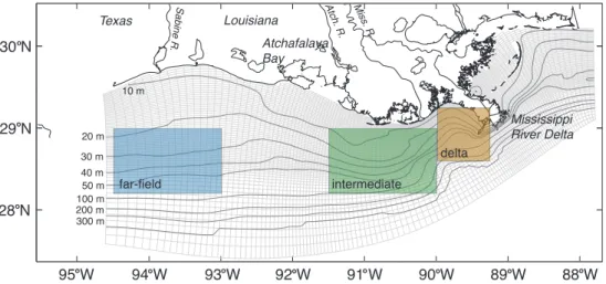
Fig. 1. Model domain and bathymetry. The colored boxes indicate areas used for averaging throughout the manuscript and are referred to as delta (brown), intermediate (green) and far-field (blue) region in the text.
in Hetland and DiMarco (2008, 2011). We provide a sum-mary of the main features here. The model uses fourth-order horizontal advection of tracers, third-order upwind advection of momentum, conservative splines to calculate vertical gra-dients, and the Mellor and Yamada (1982) turbulence clo-sure scheme for vertical mixing. The model is initialized on 1 January 1990 using an average winter profile of tempera-ture and salinity calculated based on historical hydrographic data from the World Ocean Database (Boyer et al., 2006) and assumed to be horizontally uniform. We found a hor-izontally uniform initial condition to work well as most of the region is shallower than 50 m and completely homoge-nized during winter mixing. On the shelf, horizontal salin-ity gradients establish quickly (within a few weeks) after model start due to freshwater input from the Atchafalaya and Mississippi Rivers. The temperature and salinity boundary conditions use an adaptive nudging technique (Marchesiello et al., 2001) where tracers are relaxed to the horizontally uni-form monthly climatology throughout the integration with a timescale of 10 days for outgoing information and 1 day for incoming information. The western boundary (downcoast, in the direction of Kelvin wave propagation), however, uses no-gradient conditions for three-dimensional velocity and tracer information. This allows information to leave the domain with little impedance. At the other open boundaries, radi-ation conditions are used for the three-dimensional veloci-ties and tracers. A Flather (1976) condition with no mean barotropic background flow is used for the two-dimensional velocities and free surface at all open boundaries.
Our model is forced with spatially uniform but temporally varying 3-hourly winds from the BURL 1 C-MAN weather station at 28◦54′N, 89◦25′W near the major pass of the Mis-sissippi delta. Given the spatial scales of the local wind field (Wang et al., 1998), spatially uniform wind forcing is appro-priate for our model domain. Data gaps were filled using
neighboring buoys (first station 42040 located at 29◦12′N 88◦12′W, then station 42007 located at 30◦5′N 88◦46′W). We specified surface heat and freshwater fluxes using the cli-matological fields of da Silva et al. (1994a,b), and freshwa-ter inputs from the Mississippi and Atchafalaya Rivers using daily measurements of transport by the US Army Corps of Engineers at Tabert Landing and Simmesport, respectively. We did not include tides, as they are known to be small in this region (DiMarco and Reid, 1998).
The physical model realistically captures the two distinct modes of circulation over the Texas-Louisiana shelf, namely the mean offshore flow during upwelling favorable winds in summer and the mean westward (downcoast) flow dur-ing downwelldur-ing favorable winds for the rest of the year, as described in Hetland and DiMarco (2008). Hetland and DiMarco (2011) assess the hydrodynamic model skill in re-producing moored current observations, and temperature and salinity distributions based on hydrographic surveys of water masses over the shelf for the periods from 1992 to 1994 and 2004 to 2005. They defined skill as
skill=1−
PN
i=1(mi−oi)2
PN
i=1(ci−oi)2
(1)
of the currents. These analyses suggest that the model is able to reproduce the large-scale structure of the Mis-sissippi/Atchafalaya River plume over the Texas-Louisiana shelf. However, there also exists an energetic small-scale eddy field, which the model is only able to reproduce in terms of eddy variance, but not in detail. DiMarco et al. (2010) describe observations of small-scale, energetic features with spatial scales of 20–50 km.
2.2 Biological model
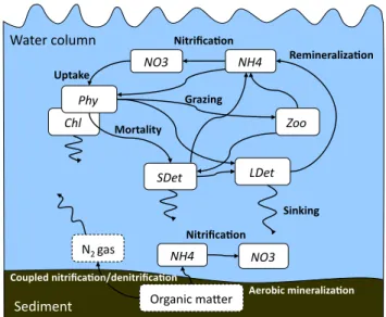
The biological component of our model uses the nitrogen cy-cle model described in Fennel et al. (2006, 2008). The model is a relatively simple representation of biological nitrogen cycling processes in the water column. It includes seven state variables: two species of dissolved inorganic nitrogen (nitrate, NO3, and ammonium, NH4), one functional
phyto-plankton group, Phy, chlorophyll as a separate state variable, Chl, to allow for photoacclimation, one functional zooplank-ton group, Zoo, and two pools of detritus representing large, fast-sinking particles, LDet, and suspended, small particles, SDet (see Fig. 2). The main processes are
1. temperature, light- and nutrient-dependent phytoplank-ton growth with ammonium inhibition of nitrate uptake, 2. zooplankton grazing represented by a Holling-type III
parameterization,
3. aggregation of phytoplankton and small detritus to fast sinking large detritus,
4. photoacclimation (i.e. a variable ratio between phyto-plankton and chlorophyll),
5. linear rates of phytoplankton mortality, zooplankton basal metabolism, and detritus remineralization, 6. a second order zooplankton mortality,
7. light-dependent nitrification (i.e. oxidation of ammo-nium to nitrate), and
8. vertical sinking of phytoplankton and detritus.
Here we only give the parameterizations for the first three processes. For other details on model justification, equations and parameters we refer the reader to Fennel et al. (2006, 2008). Similar to the model of Green et al. (2008) for the Texas-Louisiana shelf, our model does not explicitly include phosphate limitation as nitrogen is considered the dominant limiting nutrient.
The phytoplankton growth rate µ depends on tempera-tureT through the maximum growth rateµmax=µmax(T )= µ01.066T (Eppley, 1972) withµ0=0.69 d−1, on the
photo-synthetically active radiationI and on the nutrient concen-trations NO3and NH4according to
NO3
Chl
LDet
Organic ma*er N2 gas NH4
NO3
Water column
Sediment Phy
NH4
Remineraliza*on
Uptake
Nitrifica*on
Nitrifica*on Grazing
Mortality Zoo
SDet
Aerobic mineraliza*on Coupled nitrifica*on/denitrifica*on
Sinking
Fig. 2. Schematic of the biological model. State variables are
shown in solid boxes. Variables that are not explicitly included are indicated by dashed boxes.
µ=µmaxf (I )(LNO3+LNH4) (2)
where
LNO3=
NO3 kNO3+NO3
1 1+NH4/ kNH4
(3) and
LNH4= NH4
kNH4+NH4
(4)
with kNO3 =kNH4=0.5 mmol N m−3. The photosynthet-ically available light I is exponentially decreasing with depth (see Eq. 7 below). The function f (I )represents the photosynthesis-irradiance relationship (Evans and Parslow, 1985)
f (I )= αI
p µ2
max+α2I2
(5)
whereα=0.025 (W m−2)−1d−1.
The phytoplankton loss due to macrozooplankton grazing isgZoo, where the grazing rategis represented by
g=gmax
Phy2
kP+Phy2 (6)
with a maximum grazing rate gmax =
0.6 (mmol N m−3)−1d−1and a half-saturation concentration for phytoplankton ingestion ofkp=2 (mmol N m−3)2.
A first order mortality lossmpPhy is included and
The phytoplankton loss due to aggregation of phytoplank-ton and small detritus is parameterized asτ (SDet+Phy)Phy and enters the pool of fast-sinking large detritus LDet. The aggregation parameterτ is 0.01 (mmol N m−3)−1d−1.
The representation of nitrogen cycling in the water col-umn in our model is similar to other coupled models (e.g., Oschlies, 2002; Gruber et al., 2006), however, the model’s treatment of sediment remineralization, which is critical for model application to continental shelf regions, is unusual. The model uses an empirical parameterization of sediment denitrification. Specifically, organic matter that reaches the sediment is remineralized in fixed proportions through aero-bic and anaeroaero-bic remineralization. The fractions are deter-mined using the linear relationship between sediment deni-trification and oxygen consumption that Seitzinger and Gib-lin (1996, their Fig. 1) calculated for a compilation of pub-lished measurements (note that their relationship includes production of N2 gas through anammox; the term
denitri-fication is used here to denote canonical denitridenitri-fication fol-lowing Devol (2008) and includes all processes that produce N2gas). This empirical relationship was based on 50 data
points. Fennel et al. (2009) compiled a larger data set includ-ing 648 data points across a range of aquatic environments, including from the coastal Gulf of Mexico, and reevaluated the linear regression. This new relationship deviates little from the previously published one, although the coefficient of determination for the larger data set is smaller than that of Seitzinger and Giblin (1996). Using the linear relation-ship between sediment oxygen consumption and denitrifica-tion, the stoichiometries for aerobic remineralizadenitrifica-tion, deni-trification and nideni-trification, and the assumptions that organic matter is remineralized instantaneously and that denitrifica-tion occurs through coupled nitrificadenitrifica-tion-denitrificadenitrifica-tion only, the fraction of remineralization that occurs through denitrifi-cation can be calculated. Essentially one assumes that sedi-ment oxygen consumption results from aerobic remineraliza-tion and nitrificaremineraliza-tion only. The details of this calcularemineraliza-tion are given in Fennel et al. (2006) and are not repeated here for the sake of brevity.
In combination with the freshwater discharge described above, the model receives inorganic and organic nutri-ents. Specifically nitrate, ammonium and particulate ni-trogen fluxes (the latter is assumed to enter the pool of small detritus in the model) are specified (Fig. 3) based on monthly nutrient flux estimates from the US Geological Sur-vey (Aulenbach et al., 2007). Particulate organic nitrogen fluxes are determined as the difference between total Kjel-dahl nitrogen and ammonium.
In order to account for light attenuation in the river plume due to colored dissolved organic matter and suspended ter-rigenous sediments we introduced a salinity-dependent atten-uation term in the calculation of the photosynthetically active radiationIat depthzas follows
I (z)=I0·par·e−zK−zKsalt−Kchl
Rz
0Chl(ζ )dζ, (7)
whereI0is the incoming light just below the sea surface, par
is the fraction of light that is available for photosynthesis, and
KandKchlare the light attenuation coefficients for water and
chlorophyll, respectively. The salinity-dependent attenuation isKsalt=max(−0.024S+0.89,0)whereSis salinity.
Here, we present a 15-yr simulation starting on 1 January 1990 and ending on 31 December 2004. The biological vari-ables NH4, Phy, Chl, Zoo, SDet and LDet were initialized
with small constant values. NO3was initialized with a
hori-zontally homogenous mean winter profile based on data from the World Ocean Database (Boyer et al., 2006). As with tem-perature and salinity, we found a horizontally uniform nitrate profile to work well for initialization as model spin-up time is short (a few weeks) and horizontal nitrate gradients estab-lish quickly due to nitrogen inputs from the Mississippi and Atchafalaya Rivers. At the open boundaries climatological NO3distributions were prescribed using measurements from
the LATEX and NEGOM cruises (Nowlin Jr. et al., 1998; Jochens et al., 2002). All other biological state variables at the boundary are set to small positive values.
3 Results
Here we describe key features of the simulated biological variables, focusing primarily on nutrients and phytoplank-ton, and compare simulated variables and rates to available observations. We first compare simulated surface nitrate and chlorophyll distributions and vertically integrated rates of primary production to observations, then describe the cli-matological seasonal cycle of simulated nitrate, phytoplank-ton and zooplankphytoplank-ton for three sub-regions of the model do-main, which represent an ecological gradient, and then com-pare simulated phytoplankton growth, zooplankton grazing and organic matter sedimentation rates to observational esti-mates.
3.1 Surface nitrate concentrations
First we show simulated surface nitrate concentrations plot-ted over salinity and in comparison to observations by Syl-van et al. (2006) in order to illustrate typical patterns of this property; then we present a more quantitative comparison of surface nitrate with observations.
Fig. 3. (a) Climatological daily nitrate input from the Mississippi River (thick black line) and one standard deviation (gray area) for the period from 1990 to 2004. The daily nitrate input is also shown for the years of highest (1993, solid black line) and lowest (2000, dashed line) discharge. (b) Annual means of Mississippi River freshwater discharge (dark gray bars) and nitrate input (light gray bars). Mean freshwater discharge and nitrate input was lower for the years 1999 to 2004 with an average of 4.4×10¹¹m3yr−1and 4.5×10¹⁰mol N−1yr−1, respectively, than during the years 1990 to 1998 with 5.3×10¹¹m3yr−1and 5.7×10¹⁰mol N−1yr−1. Average annual discharges for both periods are shown as solid horizontal lines.
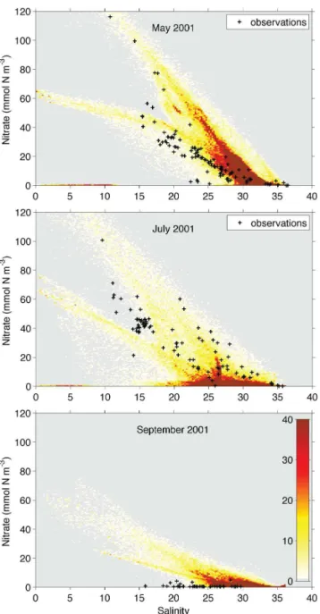
(>32) in May. Over the course of the summer, surface ni-trate is drawn down at intermediate salinities and generally more variable. By September of 2001 all samples at interme-diate salinities have low nitrate concentrations (Fig. 4, sym-bols in bottom panel). The simulated nitrate patterns are sim-ilar to the observations in terms of their monthly evolution. As seen in the observations, the simulated surface nitrate concentrations resemble a conservative mixing relationship most closely in May, and the different river end member con-centrations from the Mississippi and Atchafalaya Rivers are clearly distinguishable (Fig. 4, top panel). Over the course of the summer, nitrate is drawn down at intermediate salinities, and consistently low by September.
For a more quantitative comparison we obtained all avail-able surface nitrate observations for our study region from the World Ocean Database (Boyer et al., 2006) (the majority of the additional data is from LUMCON’s hypoxia monitor-ing program; see, for example, Rabalais et al., 2002). We binned all surface nitrate data that fall into the delta and in-termediate regions (defined in Fig. 1) by month (no data were
Fig. 4. Simulated surface nitrate concentrations are shown over salinity in form of a 2-dimensional histogram. All surface cells in the model domain are included. Color indicates the number of sim-ulated nitrate-salinity-pairs per bin (see color scale in bottom right panel). Symbols represent surface nitrate observations for the same months.
3.2 Surface chlorophyll and primary production We now compare the simulated surface chlorophyll to obser-vations derived from the SeaWiFS satellite. First we show the spatial distribution of monthly means from 1998 to 2004 (i.e. when the simulation period overlaps with the SeaWiFS period) in Fig. 6. Chlorophyll concentrations are observed to be highest in the freshwater plumes (>30 mg m−3) and
show a generally decreasing tendency from high concentra-tions near shore (1 to 10 mg m−3) to values<1 mg m−3near
the shelf break (Fig. 6).
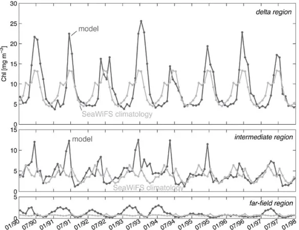
More quantitative comparisons for the subregions defined above are presented in Figs. 7, 8 and 9. Since only the sec-ond part of our simulation overlaps with the SeaWiFS obser-vations, we split the comparison into two periods: (1) Jan-uary 1990 to December 1997 for which we use the monthly SeaWiFS climatology (Fig. 7), and (2) January 1998 to De-cember 2004 for which we use monthly SeaWiFS means for the specific year (Figs. 8 and 9). In general chlorophyll con-centrations are lowest in winter, increase in spring, remain high throughout summer, and decrease in early fall (Fig. 6). For the first period shown in Fig. 7, the model tends to over-estimate the observations in all three regions , which is not surprising as nitrogen loads were markedly higher from 1990 to 1998 compared to most of the SeaWiFS data period from 1999 to 2004 (see Fig. 3). In the delta region the model repro-duces the climatology best in the years 1992 and 1994, which were similar in terms of freshwater discharge and nutrient in-put to the SeaWiFS years. The largest summer chlorophyll concentrations are predicted for 1993 (the year with highest discharge and nitrogen load). For the intermediate region, the range and temporal evolution of chlorophyll agrees well with the climatology, in particular for the years 1992 and 1996 to 1998. In 1993 the model predicts higher than av-erage chlorophyll concentrations as one would expect given the disproportionate nitrogen load that year. Also, the oc-casionally elevated chlorophyll values in summer are likely due to the larger nitrogen loads, especially for the first half of the simulation period. For the far-field region the model-simulated values agree well with the climatology from 1995 through 1998, i.e. the years when Mississippi River nitrogen loads were closer to loads observed during our SeaWiFS data period, while concentrations are above the climatology from 1990 to 1994.
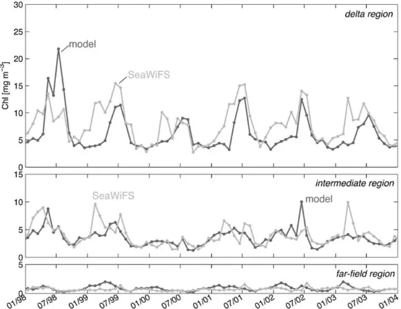
For the period where the simulation overlaps with the Sea-WiFS record (1998 to 2004; shown in Fig. 8) the amplitude of simulated chlorophyll agrees much better with the obser-vations in all three regions. In the delta region, the model overestimates chlorophyll in summer of 1998, but repro-duces observed chlorophyll closely in the summers of 1999 to 2004. Chlorophyll accumulation in spring is delayed in the model compared with the observations, as was appar-ent also in the climatological comparison in Fig. 7. In the intermediate region, the model is tracking seasonal and in-terannual variations well without any systematic differences (Fig. 8), although the model occasionally over- and underes-timates the observations, e.g. in February 1999, June 2002 and March 2003. In the far-field region the simulated chloro-phyll is close to observations (Fig. 8) and consistently lower than during the years with higher discharge from 1990 to 1994 (see Fig. 7).
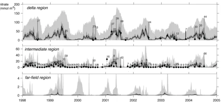
Fig. 5. Median (thick line), range between 25th and 75th percentiles (dark gray) and range between minimum and maximum simulated surface nitrate in the delta, intermediate and far-field regions (defined in Fig. 1) and corresponding median (dots), range between 25th and 75th percentiles (thick vertical lines) and range between minimum and maximum values (thin vertical lines) of monthly binned observations. The number of observations in each monthly bin is shown near each maximum value.
April June July September
model
SeaWiFS
SeaWiFS log(chl)
model log(chl)
-1 0 1 2
-1 0 1 2
April May June July August September
100
0 20 40 60 80 Chl (mg m ) 0.01 1 >30
-3
corr = 0.49 corr = 0.55 corr = 0.65 corr = 0.64 corr = 0.65 corr = 0.64
Fig. 7. Monthly mean surface chlorophyll concentrations for January 1990 to December 1997 in comparison with the monthly SeaWiFS climatology, both averaged over the delta, intermediate and far-field regions.
simulated values in Fig. 9. The corresponding coefficient of determination is 64 %, which is encouraging. It should be noted here that no systematic parameter tuning or formal parameter optimization was performed.
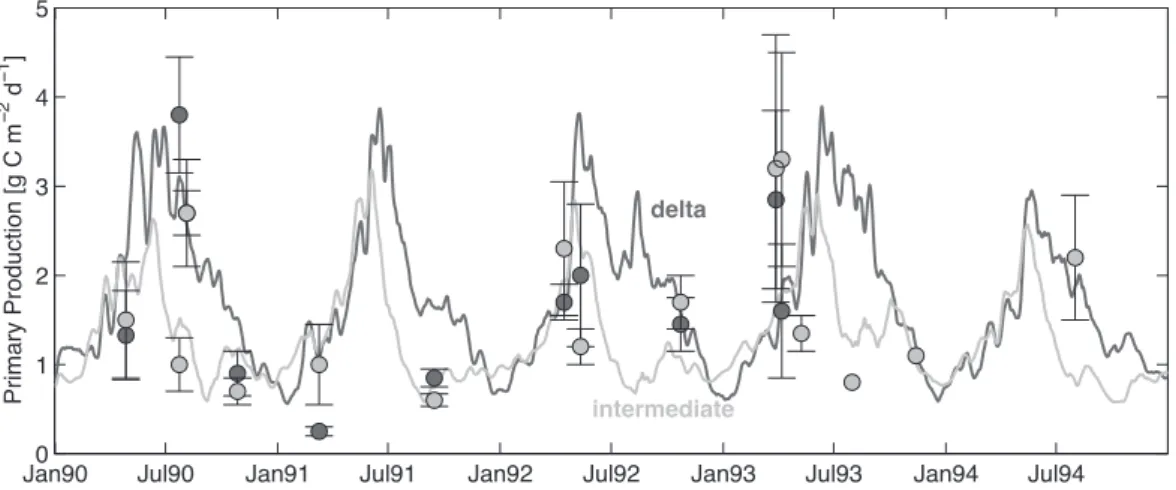
We also compared simulated rates of primary production (µPhy), averaged for the delta and intermediate regions, to the observations of Lohrenz et al. (1997) (Fig. 10). The sim-ulated rates were calcsim-ulated assuming a constant C-to-N ratio of 106:16 (as is commonly done in nitrogen-based models). Observed rates range from typically∼1 g C m−2d−1in fall
or winter to maximum values between 3 and 4 g C m−2d−1
during spring and summer, but are highly variable, as indi-cated by the large standard deviations associated with some values and the large differences in observations made only a few days apart (e.g. in spring of 1993). The simulated rates agree with the observations in terms of magnitude and tem-poral patterns; they agree especially well in 1990 and 1992. The small observed primary production value for the delta region in early 1991 seems unrealistically low (it is much smaller than primary production in the intermediate region) and is likely not an adequate representation of the mean pri-mary production for the delta region.
3.3 Seasonal cycle of nitrate, phytoplankton and zooplankton
Fig. 8. Monthly mean surface chlorophyll concentrations in comparison with the monthly SeaWiFS means for January 1998 to December 2004, both averaged over the delta, intermediate and far-field regions.
from April to October (by∼25 mmol N m−3) through dilu-tion (i.e. export of nitrate across the delta region’s boundary) and phytoplankton uptake, and nitrate is replenished again during the other months of the year through river input and, to a lesser degree, remineralization. Average nitrate concen-trations in the intermediate region are near 10 mmol N m−3 during winter and early spring but drop to limiting concen-trations between April and July, and remain low for the fol-lowing 4 to 5 months. In the far-field region, average mixed layer nitrate is always at limiting concentrations.
Average mixed layer phytoplankton biomasses in the delta and intermediate regions are near 2 mmol N m−3 from De-cember to March and begin to increase and diverge in April, reaching maximum concentrations of 7 mmol N m−3 in the delta region in July and 3.5 mmol N m−3in the intermediate
region (Fig. 12). In contrast, maximum zooplankton con-centrations are very similar (∼4 mmol N m−3in June) in the
delta and intermediate regions and remain similar through-out the whole seasonal cycle. In the far-field region, average mixed layer phytoplankton biomass is almost stationary near 1 mmol N m−3, while zooplankton biomass exhibits a sea-sonal cycle with increasing concentrations in spring. Here the phytoplankton standing stock is supported by recycled production. During spring and early summer, average mixed
layer zooplankton biomass exceeds that of phytoplankton in the far-field region.
3.4 Phytoplankton growth rates
0 5 10 15 20 25 0
5 10 15 20 25
model chlorophyll (mg m−3)
SeaWiFS chlorophyll (mg m
−
3)
R2 = 0.64
Fig. 9. Monthly mean SeaWiFS chlorophyll concentrations from January 1998 to December 2004 plotted over simulated surface chlorophyll; both averaged over the delta (brown dots), interme-diate (green dots) and far-field (blue dots) regions. Errorbars in-dicate one standard deviation. The 1-to-1 line is shown as black line. Coefficient of determination, defined asR2=1−SSerr
SStot with
the total sum of squares SStot=P
i(oi− ¯o)2, the residual sum of squares SSerr=P
i(mi−oi)2, monthly mean observed valuesoi, and monthly mean model valuesmi, is given.
remarkably well with the model simulated growth rates of 0.5 d−1 for the delta region and 0.7 d−1 for the intermedi-ate region for March 1991 (not shown). The observed mean and median growth rates for July/August 1990 were 1.3 and 1.0 d−1, which also agree very well with the simulated rates of 1.1 d−1for July 1990 and 0.8 d−1for August 1990 in the delta region (not shown).
3.5 Zooplankton grazing and other loss terms
The zooplankton variable in our model is assumed to pri-marily represent macrozooplankton such as copepods, which have lower growth rates than phytoplankton during bloom conditions and thus lag behind phytoplankton in spring. Mi-crozooplankton, however, grow at similar rates as small toplankton and are thus able to respond to increasing phy-toplankton concentrations without delay. These microzoo-plankton grazers are not represented explicitly in our model, however, the first order mortality loss of phytoplankton can be interpreted to represent the grazing loss of microzooplank-ton. This first order mortality loss (represented bymPPhy) is
largest in May, June and July in the delta region with mean values of 50–70 mg C m−2d−1, and smaller by about half in
the intermediate region (Fig. 14e). The first order mortality loss is much smaller in the far-field region with summer rates of about 10 mg C m−2d−1.
The macrozooplankton grazing losses (represented by
gZoo) are higher than the first order, microzooplankton graz-ing losses with mean values of about 120–150 mg C m−2d−1 in May and June in the delta and intermediate regions, and between 30–40 mg C m−2d−1 in the far-field region (Fig. 14a). These rates can be compared with the copepod grazing rates determined by Dagg (1995), who estimated daily ingestion rates of 537 and 92 mg C m−2d−1 at sta-tions in the delta and intermediate regions, respectively, in September of 1991, and 166 and 147 mg C m−2d−1 at the same stations in May of 1992. Both, the May 1992 rates and the September 1991 intermediate region rate, are similar to the model-simulated mean rates. The rate observed in the delta region in September 1991 (537 mg C m−2d−1) is much
higher than the model-simulated mean rate for the region, which may in part be due to averaging (the simulated daily rates reached values up to 320 mg C m−2d−1).
The simulated monthly mean aggregation rates (repre-sented byτ (SDet+Phy)), which are indicative of the sedi-mentation flux, range between 0.1 and 0.45 d−1in the delta region and between 0.05 and 0.25 d−1in the intermediate re-gion (note that aggregation losses, i.e.τ (SDet+Phy)Phy, are given in Fig. 14c). Fahnenstiel et al. (1995) estimated taxon-specific sedimentation rates between<0.001 and 1.0 d−1in the delta and intermediate region and found the largest sedi-mentation fluxes associated with diatoms. While these rates are not representative of the phytoplankton community and thus cannot be compared directly to the model-simulated rates it is worthwhile noting that the model-simulated rates are within the observed range. Aggregation loss has the most pronounced spatial dependence of all three biological loss terms. In the delta region, aggregation loss is similar in mag-nitude to the combined grazing and mortality losses. In the intermediate region, aggregation loss is similar to the first order mortality losses, but much smaller than the macrozoo-plankton grazing term. In the far region, aggregation loss makes up less than half of the first order mortality term and both are much smaller then macrozooplankton grazing.
4 Discussion
Jan900 Jul90 Jan91 Jul91 Jan92 Jul92 Jan93 Jul93 Jan94 Jul94 1
2 3 4 5
Primary Production [g C m
−2 d −1 ]
delta
intermediate
Fig. 10. Simulated primary production averaged for the delta and intermediate regions (solid lines) compared to measurements by Lohrenz et al. (1997) for the same regions (filled circles with errorbars represent mean and standard deviation). The dark and lights gray symbols and lines correspond to the delta and intermediate regions, respectively.
delta, intermediate and far-field regions and contrast the rel-ative importance of different phytoplankton losses in these regions. We then examine relationships between monthly mean primary production in the delta region and Mississippi River nitrate load in order to elucidate why primary produc-tion in this region is correlated with nitrate load even though phytoplankton growth is not limited by nitrate.
4.1 Factors controlling plankton growth and accumulation of biomass
In order to investigate which factors limit phytoplankton growth in the three regions, we calculated the mixed layer mean light-limitation termf (I )and show its climatological monthly means for the 15-yr simulation period in Fig. 13b. Small values off (I )indicate light-limitation, while values near 1 correspond to no light-limitation. We also calculated the mixed layer mean values of the nutrient-limitation term
LTOT=LNO3+LNH4 and show its climatological monthly means in Fig. 13c. Again, values of LTOT near 1
corre-spond to no nutrient-limitation, while small values indicate nutrient-limitation.
As expected, light-limitation is strongest in the delta and weakest in the far-field region. There is a pronounced sea-sonal cycle to the light-limitation term that is coherent in all three regions with strongest light-limitation in late fall and winter and lowest light-limitation in early summer. Except for fall, where light-limitation in the intermediate and far-field regions is of similar magnitude, there is always a pro-nounced spatial gradient with strongest light-limitation in the delta region and weaker light-limitation in the interme-diate and far-field regions. The patterns of nutrient limita-tion are opposite in many respects. There is essentially no nutrient-limitation in the delta region; nutrient-limitation in-creases toward the intermediate and far-field regions. In all three regions nutrient-limitation is more pronounced in the
fall and weakest in the spring. The ratio off (I )andLTOT
(Fig. 13d) can be interpreted as a measure of the relative importance of light- versus nutrient-limitation (small values correspond to light-limitation) and illustrates that the delta region is strongly light-limited all year, while the far-field re-gion is strongly nutrient-limited in summer, and the interme-diate region is midway between the two. Seasonal changes in this ratio are small in the delta region, and most pronounced in the far-field region where limitation by light becomes more important in winter. The phytoplankton growth rate is de-termined by the product of f (I )andLTOT, which largely compensate for each other across the spatial gradient, and is modulated only by the temperature-dependent value of the maximum growth rate, which is very similar in all three re-gions and contributes to the pronounced seasonal cycle in phytoplankton growth rates (Fig. 13a).
The phytoplankton growth rate in the delta region is lower than in the intermediate region from October through July, yet, phytoplankton biomass and primary production are higher in the delta region (by a factor of 2 in July). It can be inferred that the spatial structure in phytoplankton loss terms contributes significantly to the regional differences in phyto-plankton accumulation.
In the geographic regions considered here, phytoplankton can be lost by physical transport across the region bound-aries and by biological losses (i.e. grazing-induced mortality, sinking). The sum of the climatological biological loss terms (described individually in Sect. 3.5 above; shown in Fig. 14d) varies between a minimum of 20–40 mg C m−2d−1in winter
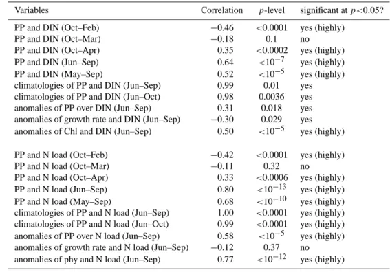
Table 1. Linear correlation coefficients andp-levels for the delta region.
Variables Correlation p-level significant atp<0.05?
PP and DIN (Oct–Feb) −0.46 <0.0001 yes (highly)
PP and DIN (Oct–Mar) −0.18 0.1 no
PP and DIN (Oct–Apr) 0.35 <0.0002 yes (highly)
PP and DIN (Jun–Sep) 0.64 <10−7 yes (highly)
PP and DIN (May–Sep) 0.52 <10−5 yes (highly)
climatologies of PP and DIN (Jun–Sep) 0.99 0.01 yes
climatologies of PP and DIN (Jun–Oct) 0.98 0.0036 yes
anomalies of PP over DIN (Jun–Sep) 0.31 0.018 yes
anomalies of growth rate and DIN (Jun–Sep) −0.30 0.029 yes
anomalies of Chl and DIN (Jun–Sep) 0.50 <10−5 yes (highly)
PP and N load (Oct–Feb) −0.42 <0.0001 yes (highly)
PP and N load (Oct–Mar) −0.11 0.32 no
PP and N load (Oct–Apr) 0.33 <0.0006 yes (highly)
PP and N load (Jun–Sep) 0.80 <10−13 yes (highly)
PP and N load (May–Sep) 0.68 <10−10 yes (highly)
climatologies of PP and N load (Jun–Sep) 1.00 <0.0001 yes (highly) climatologies of PP and N load (Jun–Oct) 0.99 <0.0001 yes (highly) anomalies of PP over N load (Jun–Sep) 0.58 <10−5 yes (highly) anomalies of growth rate and N load (Jun–Sep) −0.12 0.37 no
anomalies of phy and N load (Jun–Sep) 0.77 <10−12 yes (highly)
of production and losses, which is shown in Fig. 14f for pri-mary production and biological losses (i.e. the difference be-tween Fig. 14b and d).
In the delta region, there is a positive imbalance from April to July reaching a maximum of about 60 mg C m−2d−1 in
June. In May and June this imbalance corresponds to about 10 % of primary production, in other words, roughly 10 % of primary production can accumulate while about∼90 % is lost to grazing, mortality and sinking. During the rest of the year the phytoplankton standing stock is in balance or declin-ing (the imbalance between primary production and biologi-cal losses is near zero or negative).
In the intermediate region, the imbalance of primary pro-duction and biological losses is negative most of the year, approaching zero only in winter, despite the accumulation of phytoplankton in spring when it is doubling its standing stock compared to winter values (Fig. 12). We infer that advection and mixing of phytoplankton results in a net transport from the delta to the intermediate region supporting the accumula-tion of phytoplankton biomass in the latter. A similar picture emerges for the far-field region, where primary production and biological losses are in balance for most of the year, ex-cept during spring and early summer when biological losses exceed primary production, while the phytoplankton stand-ing stock is increasstand-ing slightly. This indicates that physical transport of phytoplankton into the far-field region occurs at this time.
In summary, small mismatches between primary produc-tion and phytoplankton losses can explain the pronounced regional differences in phytoplankton standing stock and pri-mary production that are observed to occur between the delta, intermediate and far-field region.
4.2 Correlations between primary production and nutrients for the delta region
Analysis of the limitation terms on phytoplankton growth (Fig. 13; previous section) indicates that phytoplankton growth in the delta region is not limited by nitrate in our model. This is also in agreement with observations by Lohrenz et al. (1999) that indicate phytoplankton is light-limited in this region. Yet, a correlation between Mississippi nitrogen load and primary production has been shown to ex-ist for this region by Lohrenz et al. (1997) and, more recently based on a larger data set, by Lehrter et al. (2009). The ex-istence of this correlation is often interpreted as a bottom up effect of river nutrients directly stimulating primary produc-tion, which appears to be in contradiction with the observed lack of nutrient limitation. Our model simulation allows us to examine the nature of this relationship in more detail.
First, we examine the relationship between monthly mean primary production in the delta region and monthly NO3
2 4 6 8 10 12 0
10 20 30 40
NO
3
(mmol m
−3 )
2 4 6 8 10 12
0 1 2 3 4 5 6 7
Phytoplankton biomass (mmol N m
−3 )
2 4 6 8 10 12
0 1 2 3 4
Calendar month
Zoooplankton biomass (mmol N m
−3 )
delta
intermediate
far-field
Fig. 11. Climatological monthly means of simulated mixed layer depth (top) and surface salinity (bottom) for the delta, intermediate and far-field regions (see Fig. 1).
a statistically significant linear relationship between monthly primary production and monthly NO3 load with a slightly
negative slope. In other words, during this period primary production is essentially insensitive to NO3load. From May
through September a different and statistically significant re-lationship emerges with a positive slope. During this period, primary production is elevated when NO3load and, by
im-plication, surface DIN concentrations are high (Fig. 15a, the same pattern emerges when primary production is related to monthly mean DIN concentrations in the delta region instead of NO3load; see Table 1). In other words, the system shifts
2 4 6 8 10 12
0 10 20 30 40 50
Mixed layer depth (m
)
2 4 6 8 10 12
20 25 30 35 40
Calendar month
Surface salinity
delta intermediate
far-field
Fig. 12. Climatological monthly means of simulated mixed layer nitrate (top), phytoplankton (middle) and zooplankton (bottom) biomasses for the delta, intermediate and far-field regions (see Fig. 1).
from a phase of insensitivity to NO3load (or DIN
concentra-tion) in winter and early spring to a phase when primary pro-duction appears to be sensitive to NO3load in late spring and
summer. The shift occurs in March-April when phytoplank-ton growth rates are already near their maximum values.
This bi-modal pattern supports the previously reported re-lationships, which focused on spring and summer, i.e. one of the two distinct periods we identified. Lohrenz et al. (1997) used data primarily from late spring and summer in their analysis; no data points for winter and only one early fall data point were included and their only measurement from early spring (March 1991) was excluded (otherwise the resulting relationship was not significant). Lehrter et al. (2009) re-peated the analysis after adding 7 more data points (all spring and summer observations) and again found a significant rela-tionship, although with a much smallerR2=0.20 instead of
R2=0.58 in Lohrenz et al. (1997).
2 4 6 8 10 12 0
0.2 0.4 0.6 0.8 1 1.2 1.4
Growth rate (d
−1 )
2 4 6 8 10 120
0.2 0.4 0.6 0.8 1
Light−limitation term: f(I)
2 4 6 8 10 12
0 0.2 0.4 0.6 0.8 1
Calendar month
Nutrient−limitation term: L
tot
2 4 6 8 10 120
0.5 1 1.5 2
Calendar month
Ratio of f(I):L
tot
a) b)
c)
d)
no limitation
limitation
no limitation
limitation
nutrient-limitation
light-limitation
far-field far-field
intermediate intermediate
delta
delta
Fig. 13. Monthly climatology of simulated mixed layer mean phytoplankton growth rate (a), light-limitation term (b), nutrient-limitation term (c) and ratio of light- and nutrient-limitation (d) for the delta, intermediate and far-field regions.
production and NO3 load (or DIN concentration) have
sea-sonal cycles. In fact, similar significant correlations result when the average seasonal cycle of primary production and NO3load (or DIN concentration) is used (Table 1). We thus
removed the annual cycle from the time series of monthly primary production and NO3load (and DIN concentration)
and investigated the resulting anomalies for positive corre-lations (Fig. 15b). A highly significant positive correlation (p<10−5) between primary production anomalies and NO3
load anomalies for the period from June through September emerges. In other words, interannual differences in NO3load
are reflected in variations in primary production in summer (not in spring). However, when investigating the monthly mean growth rate anomalies of the phytoplankton commu-nity, no significant relationship with NO3 load anomalies
(and DIN concentration anomalies) exists (Fig. 15c). The lack of a relationship between nutrient load (or concentra-tion) and community growth rates is consistent with our ex-pectation that a phytoplankton community that is not limited by nutrients also should not be sensitive to perturbations in nutrient concentrations. Considering that primary production is the product of instantaneous phytoplankton growth rate and accumulated phytoplankton biomass, the relationship be-tween primary production and NO3load could simply reflect
a relationship between accumulated phytoplankton biomass and NO3 load (or concentration). In fact, there is a highly
significant relationship (p<10−13) between monthly
phyto-plankton biomass anomalies and NO3load for June through
September (Fig. 15d). Thus, the positive correlation between primary production and NO3load in the light-limited region
of the plume results primarily from increased accumulation of phytoplankton in years with higher discharge and N input, possibly due to differences in loss terms (i.e., advection and mixing, grazing and sedimentation).
For example, changes in freshwater input likely cause al-tered circulation patterns over the shelf. Increased accu-mulation during anomalously high streamflow years (corre-sponding to high NO3load because NO3load and streamflow
2 4 6 8 10 12 0
50 100 150 200
Grazing loss (mg C
m
−2 d −1 )
2 4 6 8 10 120
100 200 300 400 500
PP (mg C
m
−2 d −1 )
2 4 6 8 10 12
0 50 100 150 200
Aggregation loss (mg C
m
−2 d −1 )
2 4 6 8 10 120
100 200 300 400
Sum of losses (mg C
m
−2 d −1 )
2 4 6 8 10 12
0 50 100 150 200
Calendar month
Mortality loss (mg C
m
−2 d −1 )
2 4 6 8 10 12−20
0 20 40 60
Calendar month
PP − losses (mg C
m
−2 d −1)
a) b)
c) d)
e) f) delta
delta
far-field far-field
intermediate
Fig. 14. Monthly climatology of simulated mixed layer mean phytoplankton loss due to grazing (a), aggregation (c), and mortality (e). Also shown is monthly mixed layer mean primary production (b), sum of the three biological phytoplankton loss terms (d) and balance of primary production and biological loss terms (f). The losses were converted from units of mmol N m−3to mg C m−3assuming the Redfield ratio of 106C to 16N and using the molar mass of nitrogen.
conditions is beyond the scope of this paper, and will be the focus of future studies.
5 Conclusions
We presented a 15-yr simulation of a realistic physical-biological model for the Texas-Louisiana Shelf. Our model describes the spatial and temporal patterns of nitrate and phy-toplankton in agreement with observations and predicts rates of primary production and grazing that agree with experi-mentally determined rates. In the model, differences in phy-toplankton biomass and primary production across the eco-logical gradient from the delta, via the intermediate, to the
far-field region appear to be driven primarily by differences in phytoplankton losses. For example, while phytoplank-ton growth rates are systematically lower in the delta region compared to the intermediate region, phytoplankton biomass and primary production is markedly higher. This can be ex-plained by differences in the phytoplankton loss terms.
0 2 4 6 8 10 12
0 100 200 300 400 500 600 700 800
Monthly NO3 load from Mississippi (109 mol N)
Monthly mean PP (mg C m
−2 d −1)
Jan Feb Mar Apr May Jun Jul Aug Sep Oct Nov Dec
−4 −2 0 2 4 6
−300 −200 −100 0 100 200 300
Monthly NO3 load anomaly (109 mol N)
Monthly mean PP anomaly (mg C m
−2 d −1 )
−6 −4 −2 0 2 4 6
−0.4 −0.2 0 0.2 0.4 0.6 0.8
Monthly NO3 load anomaly (109 mol N)
Monthly mean growth rate anomaly (d
−1)
−6 −4 −2 0 2 4 6 8−4
−3 −2 −1 0 1 2 3 4 5 6
Monthly NO
3 load anomaly (10
9 mol N)
Monthly mean phytoplankton anomaly (mmol N m
−3 ) Jun
Jul Aug Sep
Jun Jul Aug Sep Jan
Feb Mar Apr May Jun Jul Aug Sep Oct Nov Dec
a)
b)
c)
d)
Fig. 15. Simulated monthly mean variables for the delta region plotted over monthly NO3load from the Mississippi River for the simulation
period from January 1990 to December 2004. (a) Primary production over NO3load (colored dots) and their linear regressions (solid lines) for June through September (red), May through September (magenta) and October through February (black). (b) Anomaly of primary production over anomaly of NO3load for June through September (colored dots) and their linear regression (red line). (c) Anomaly of phytoplankton growth rate over anomaly NO3load. (d) Anomaly of phytoplankton biomass over anomaly of NO3load (colored dots) and their linear regression (red line). Regression parameters are given in Table 1.
practical with sparse observational data sets, take into ac-count the autocorrelation between primary production and nitrogen load by increasing the degrees of freedom and ad-justing the p-levels appropriately. We find a statistically significant relationship between anomalies of primary pro-duction and nitrogen load for the months of June through September. We also find a statistically significant relation-ship between the anomalies of phytoplankton biomass and nitrogen load for the same months, but not for the anoma-lies of phytoplankton growth rates and nitrogen load. Since primary production is the product of growth rate and phy-toplankton biomass the relationship between primary pro-duction and nitrogen load simply reflects the relationship
between phytoplankton biomass and nitrogen load, which re-sults from differences in phytoplankton accumulation likely due to differences in loss terms.
Acknowledgements. We thank Jason Sylvan and James Ammerman
for making their nutrient data available to us and John Lehrter, Mike Dagg and two anonymous reviewers for their constructive criticism on an earlier version of this manuscript. This work was supported by NOAA CSCOR grants NA06N0S4780198 and NA09N0S4780208 and Cooperative Agreement M07AC12922 with the US Department of the Interior (Minerals Management Service). NOAA NGOMEX publication no. 141.
References
Aulenbach, B., Buxton, H., Battaglin, W., and Coupe, R.: Stream-flow and nutrient fluxes of the Mississippi-Atchafalaya River Basin and subbasins for the period of record through 2005, Open-file report 2007-1080, US Geological Survey, 2007.
Bianchi, T., DiMarco, S., Smith, R., and Schreiner, K.: A gra-dient of dissolved organic carbon and lignin from Terrebonne-Timbalier Bay estuary to the Louisiana shelf (USA), Mar. Chem., 117, 32–41, 2009.
Bianchi, T., DiMarco, S., Cowan Jr., J., Hetland, R., Chapman, P., Day, J., and Allison, M.: The science of hypoxia in the Northern Gulf of Mexico: a review, Sci. Total Environ., 408, 1471–1484, 2010.
Boyer, T. P., Antonov, J. I., Garcia, H. E., Johnson, D. R., Locarnini, R. A., Mishonov, A. V., Pitcher, M. T., Baranova, O. K., and Smolyar, I. V.: World Ocean Database 2005, edited by: Levitus, S., NOAA Atlas NESDIS 60, US Government Printing Office, Washington, DC, 190 pp., DVDs, 2006.
da Silva, A., Young-Molling, C., and Levitus, S.: Atlas of surface marine data 1994, vol. 3. Anomalies of fluxes of heat and mo-mentum, NOAA Atlas NESDIS 8, Natl. Oceanic and Atmos. Ad-min., Silver Spring, MD, 1994a.
da Silva, A., Young-Molling, C., and Levitus, S.: Atlas of sur-face marine data 1994, vol. 4, Anomalies of fresh water fluxes, NOAA Atlas NESDIS 9, Natl. Oceanic and Atmos. Admin., Sil-ver Spring, MD, 1994b.
Dagg, M.: Copepod grazing and the fate of phytoplankton in the Northern Gulf of Mexico, Cont. Shelf Res., 15, 1303–1317, 1995.
David, M., Drinkwater, L., and McIsaac, G.: Sources of nitrate yields in the Mississippi River Basin, J. Environ. Qual., 39, 1657–1667, 2010.
Devol, A. H.: Denitrification including anammox, chapt. 6: in: Ni-trogen in the Marine Environment, edited by: Capone, D., Car-penter, E., Mullholland, M., and Bronk, D., Elsevier, Burlington, Amsterdam, San Diego, London, 263–302, 2008.
DiMarco, S. and Reid, R.: Characterization of the principal tidal current constituents on the Texas-Louisiana shelf, J. Geophys. Res., 103, 3093–3109, 1998.
DiMarco, S., Chapman, P., Walker, N., and Hetland, R.: Does lo-cal topography control hypoxia on the Eastern Texas-Louisiana shelf?, J. Marine Syst., 80, 25–35, 2010.
Eldridge, P. and Roelke, D.: Origins and scales of hypoxia on the Louisiana shelf: importance of seasonal plankton dynamics and river nutrients and discharge, Ecol. Model., 221, 1028–1042, 2010.
Fahnenstiel, G., McCormick, M., Lang, G., Redalje, D., Lohrenz, S., Markowitz, M., Wagoner, B., and Carrick, H.: Taxon-specific growth and loss rates for dominant phytoplankton populations from the Northern Gulf of Mexico, Mar. Ecol.-Prog. Ser., 117, 229–239, 1995.
Fennel, K., Wilkin, J., Levin, J., Moisan, J., O’Reilly, J., and Haid-vogel, D.: Nitrogen cycling in the Middle Atlantic Bight: results from a three-dimensional model and implications for the North Atlantic nitrogen budget, Global Biogeochem. Cy., 20, GB3007, doi:10.1029/2005GB002456, 2006.
Fennel, K., Wilkin, J., Previdi, M., and Najjar, R.: Denitrification effects on air-sea CO2flux in the coastal ocean: simulations for the Northwest North Atlantic, Geophys. Res. Lett., 35, L24608,
doi:10.1029/2008GL036147, 2008.
Fennel, K., Brady, D., DiToro, D., Fulweiler, R., Gardner, W., Giblin, A., McCarthy, M., Rao, A., Seitzinger, S., Thouvenot-Korppoo, M., and Tobias, C.: Modeling denitrification in aquatic sediments, Biogeochemistry, 93, 159–178, 2009.
Flather, R.: A tidal model of the Northwest European continental shelf, Mem. Soc. R. Sci. Liege, 10, 141–164, 1976.
Fong, D. and Geyer, W.: The alongshore transport of freshwater in a surface-trapped river plume, J. Phys. Oceanogr., 32, 957–972, 2002.
Goolsby, D., Battaglin, W., Aulenbach, B., and Hooper, R.: Nitro-gen flux and sources in the Mississippi River Basin, Sci. Total Environ., 248, 75–86, 2000.
Green, R., Breed, G., Dagg, M., and Lohrenz, S.: Modeling the response of primary production and sedimentation to variable ni-trate loading in the Mississippi River plume, Cont. Shelf Res., 28, 1451–1465, 2008.
Greene, R., Lehrter, J., and Hagy, J.: Multiple regression models for hindcasting and forecasting midsummer hypoxia in the Gulf of Mexico, Ecol. Appl., 19, 1161–1175, 2009.
Gruber, N., Frenzel, H., Doney, S., Marchesiello, P., McWilliams, J., Moisan, J., Oram, J., Plattner, G., and Stolzenbach, K.: Eddy-resolving simulation of plankton ecosys-tem dynamics in the California Current Sysecosys-tem, Deep-Sea Res. Pt. I, 53, 1483–1516, 2006.
Haidvogel, D. B., Arango, H., Budgell, W. P., Cornuelle, B. D., Cur-chitser, E., Di Lorenzo, E., Fennel, K., Geyer, W. R., Hermann, A. J., Lanerolle, L., Levin, J., McWilliams, J. C., Miller, A. J., Moore, A. M., Powell, T. M., Shchepetkin, A. F., Sherwood, C. R., Signell, R. P., Warner, J. C., and Wilkin, J.: Ocean fore-casting in terrain-following coordinates: formulation and skill assessment of the regional ocean modeling system, J. Comput. Phys., 227, 3595–3624, 2008.
Hetland, R. and DiMarco, S.: How does the character of oxygen demand control the structure of hypoxia on the Texas-Louisiana continental shelf?, J. Marine Syst., 70, 49–62, 2008.
Hetland, R. and DiMarco, S.: Skill assessment of a hydrodynamic model of circulation over the Texas-Louisiana continental shelf, Ocean Modell., submitted, 2011.
Ichiye, T.: On the hydrography of the Mississippi Delta, Oceanogr. Mag., 11, 65–78, 1960.
Jochens, A., DiMarco, S., Nowlin Jr., W. D., Reid, R., and Kenni-cutt II, M.: Northeastern Gulf of Mexico chemical oceanography and hydrography study, Synthesis report, OCS study MMS 2002, Tech. rep., US Department of the Interior, Minerals Management Service, Gulf of Mexico OCS Region, New Orleans, LA, 2002. Lehrter, J., Murrell, M., and Kurtz, J.: Interactions between
fresh-water input, light, and phytoplankton dynamics on the Louisiana continental shelf, Cont. Shelf Res., 29, 1861–1872, 2009. Lohrenz, S., Fahnenstiel, G., Redalje, D., Lang, G., Chen, X., and
Dagg, M.: Variations in primary production of Northern Gulf of Mexico continental shelf waters linked to nutrient inputs from the Mississippi River, Mar. Ecol.-Prog. Ser., 155, 45–54, 1997. Lohrenz, S., Fahnenstiel, G., Redalje, D., Lang, G., Dagg, M.,
Whitledge, T., and Dortch, Q.: Nutrients, irradiance, and mix-ing as factors regulatmix-ing primary production in coastal waters impacted by the Mississippi River plume, Cont. Shelf Res., 19, 1113–1141, 1999.
boundary condition for long-term integration of regional oceanic models, Ocean Modell., 3, 1–20, 2001.
Mellor, G. and Yamada, T.: Development of a turbulence closure model for geophysical fluid problems, Rev. Geophys., 20, 851– 875, 1982.
Milliman, J. and Meade, R.: World-wide delivery of river sediment to the oceans, J. Geol., 91, 1–21, 1983.
Morse, J. and Rowe, G.: Benthic biogeochemistry beneath the Mis-sissippi River plume, Estuar. Coast., 22, 206–214, 1999. Nowlin Jr., W. D., Jochens, A. E., Reid, R. O., and DiMarco, S. F.:
Texas-Louisiana shelf circulation and transport processes study, Synthesis report. Vol. I and II. OCS study MMS 98-0035 and MMS 98-0036, Tech. rep., US Department of the Interior, Miner-als Management Service, Gulf of Mexico OCS Regional Office, New Orleans, LA, 1998.
Oschlies, A.: Improved representation of upper-ocean dynamics and mixed layer depths in a model of the North Atlantic on switching from eddy-permitting to eddy-resolving grid resolu-tion, J. Phys. Oceanogr., 32, 2277–2298, 2002.
Pe˜na, M. A., Katsev, S., Oguz, T., and Gilbert, D.: Modeling dis-solved oxygen dynamics and hypoxia, Biogeosciences, 7, 933– 957, doi:10.5194/bg-7-933-2010, 2010.
Rabalais, N., Turner, R., and Wiseman Jr., W.: Gulf of Mexico Hy-poxia, aka “The Dead Zone”, Ann. Rev. Ecol. Syst., 33, 235–263, 2002.
Rowe, G. and Chapman, P.: Continental shelf hypoxia: some nag-ging questions, Gulf Mexico Sci., 20, 153–160, 2002.
Seitzinger, S. and Giblin, A.: Estimating denitrification in North Atlantic continental shelf sediments, Biogeochemistry, 35, 235– 260, 1996.
Sylvan, J., Dortch, Q., Nelson, D., Brown, A., Morrison, W., and Ammerman, J.: Phosphorus limits phytoplankton growth on the Louisiana shelf during the period of hypoxia formation, Environ. Sci. Technol, 40, 7548–7553, 2006.
Turner, R., Rabalais, N., Swenson, E., Kasprzak, M., and Ro-maire, T.: Summer hypoxia in the Northern Gulf of Mexico and its prediction from 1978 to 1995, Mar. Environ. Res., 59, 65–77, 2005.
Walker, N. and Rabalais, N.: Relationships among satellite chlorophyll-a, river inputs, and hypoxia on the Louisiana con-tinental shelf, Gulf of Mexico, Estuar. Coast., 29, 1081–1093, 2006.
Wang, W., Nowlin Jr., W., and Reid, R.: Analyzed surface meteoro-logical fields over the Northwestern Gulf of Mexico for 1992–94: mean, seasonal, and monthly patterns, Mon. Weather Rev., 126, 2864–2883, 1998.
Wiseman Jr., W., Murray, S., Bane, J., and Tubman, M.: Physical environment of the Louisiana Bight, Contrib. Mar. Sci., 25, 109– 120, 1982.