Why recognition is rational: Optimality results on single-variable
decision rules
Clintin P. Davis-Stober
∗University of Missouri
Jason Dana
University of Pennsylvania
David V. Budescu
Fordham University
Abstract
The Recognition Heuristic (Gigerenzer & Goldstein, 1996; Goldstein & Gigerenzer, 2002) makes the counter-intuitive prediction that a decision maker utilizing less information may do as well as, or outperform, an idealized decision maker utilizing more information. We lay a theoretical foundation for the use of single-variable heuristics such as the Recogni-tion Heuristic as an optimal decision strategy within a linear modeling framework. We identify condiRecogni-tions under which over-weighting a single predictor is a mini-max strategy among a class of a priori chosen weights based on decision heuristics with respect to a measure of statistical lack of fit we call “risk”. These strategies, in turn, outperform standard multiple regression as long as the amount of data available is limited. We also show that, under related conditions, weighting only one variable and ignoring all others produces the same risk as ignoring the single variable and weighting all others. This approach has the advantage of generalizing beyond the original environment of the Recognition Heuristic to situations with more than two choice options, binary or continuous representations of recognition, and to other single variable heuristics. We analyze the structure of data used in some prior recognition tasks and find that it matches the sufficient conditions for optimality in our results. Rather than being a poor or adequate substitute for a compensatory model, the Recognition Heuristic closely approximates an optimal strategy when a decision maker has finite data about the world.
Keywords: improper linear models, recognition heuristic, single-variable decision rules.
1
Introduction
Common sense would suggest that it is always bet-ter to have more, rather than less, relevant information when making a decision. Most normative and prescrip-tive theories of multi-attribute decision making are com-pensatory models that incorporate all relevant variables. This perspective was challenged by Gigerenzer and Gold-stein (1996) and Gigerenzer, Todd, and the ABC Group (1999), who proposed a theoretical framework of sim-ple decision rules, often referred to as “fast and fru-gal” heuristics, suggesting that in some cases a decision maker (DM) utilizing less relevant information may ac-tually outperform an idealized DM utilizing all relevant information. In fact, many of these heuristics use a single cue selected among the many available for the prediction task. Key among these single-variable decision rules is the Recognition Heuristic (RH) (Gigerenzer & Goldstein, 1996; Gigerenzer et al., 1999; Goldstein & Gigerenzer, 2002).
A rapidly growing empirical literature suggests that
∗We would like to thank Dan Goldstein for generously providing
previously unpublished “German Cities” data on recognition and for comments on an early draft. Address: Clintin P. Davis-Stober, Univer-sity of Missouri at Columbia, Department of Psychological Sciences, Columbia, MO, 65211. Email: [email protected].
single-variable decision rules are descriptive for at least a subset of DMs with regard to both Take The Best (Bröder, 2000; Bröder & Schiffer, 2003; Newell & Shanks, 2003) and the RH (Goldstein & Gigerenzer, 2002; Hertwig & Todd, 2003; Pachur & Biele, 2007; Scheibehenne & Bröder, 2007; Serwe & Frings, 2006; Snook & Cullen, 2006). Questions remain, however, as to exactly when and why a single-variable rule will perform well.
Hogarth and Karelaia (2005) examined the relative per-formance of single-variable rules within a binary choice framework where both predictor (independent) and cri-terion (dependent) variable were assumed to be contin-uous. Using a combination of analytic tools and simu-lations, they found that single-variable rules have strong predictive accuracy when: 1) all predictors are highly and positively inter-correlated, 2) the single predictor used is highly (and, typically, positively) correlated with the cri-terion.1 Hogarth and Karelaia (2006) conducted a related analysis using binary rather than continuous cues (pre-dictors). Fasolo, McClelland, and Todd (2007) identified similar favorable conditions for single-variable rules us-ing a series of simulations. Shanteau and Thomas (2000) labeled environments with highly positively correlated
1In keeping with the prior literature on the recognition heuristic, we
use the term “criterion” to refer to the dependent variable of interest, e.g., the population of German cities.
predictors, “friendly” environments, and demonstrated in a simulation that single-variable rules tended to under-perform when the predictors in the model were nega-tively correlated, a finding that was later replicated by Fa-solo et al. (2007) (see also Martignon & Hoffrage, 1999; and Payne, Bettman, & Johnson, 1993). In a similar vein, Baucells, Carrasco, and Hogarth (2008) presented a framework to analyze simple decision rules within the context of cumulative dominance (see also Katsikopoulos & Martignon, 2006).
In this paper, we present results regarding the effec-tiveness of single variable rules that diverge from previ-ous studies in two major ways. First, we show that when a single predictor, denoted without any loss of general-ity,x1, is positively correlated with an array ofp-many
other predictors, where each of thesep-many predictors are either uncorrelated or weakly positively correlated, the optimal weighting scheme places greater weight on
x1 than any of the remaining cues. This result is a
ma-jor departure from previous studies (Fasolo et al., 2007; Hogarth & Karelaia, 2005; Shanteau & Thomas, 2000) that identify favorable conditions for single-variable rules as “single-factor” models where all variables are highly positively correlated. Second, our results do not rely on any specific assumptions about the cue validities, defined as the correlations between the predictors (cues) and the criterion. The only thing that matters is the sign on the correlation of the single cue. Some lexicographic single-variable rules depend upon either the knowledge or esti-mation of all cue validities. For example, the Take The Best rule (Gigerenzer & Goldstein, 1996; Gigerenzer et al., 1999) depends on the identification of the single best cue. In our results, the validity of the single variable need not be the highest among the available predictors. We apply the new results to the RH, for which Goldstein and Gigerenzer (2002) argue that the recognition validity, i.e., the correlation between the criterion and recognition, is inaccessible to the DM with the criterion variable influ-encing recognition through mediator variables in the en-vironment.
The divergence in our results stems from our somewhat different approach to answering the question “when does less information lead to better performance?” First, we characterize the RH within the framework of the linear model — i.e., within the standard regression framework — as an “estimator” that relies on a single predictor. As in the regression framework, we conceptualize the best set of weights to assign to the cues, such that if one had unlimited data and knowledge, they would maximize pre-dictive accuracy and call this vector of weightsβ. We then consider the weights that would be placed on the cues by various decision heuristics (such as equal weight-ing) as if they were estimates ofβ. Within this frame-work, we can prove results with respect to a measure
of statistical inaccuracy called “risk” (defined formally in section 2), which measures how close these heuristic weights are expected to be to the best weights,β. This measure of inaccuracy is particularly useful because it goes beyond optimizing within a single sample; the closer a set of weights is to the best weights, the more robustly it cross-validate in new samples. An advantage to cast-ing the problem within the framework of the linear model is that the results can be generalized to accommodate a broad range of situations, including choosing between more than two options, binary or continuous represen-tations of recognition, and to evaluate the success of any single variable rule, not just RH.
We show that under certain conditions, placing greater weight on a single variable relative to all others repre-sents a form of optimization: It minimizes the maximum value of risk over all choices of decision rules. As the number of cues becomes large, this mini-max strategy converges to a rule that puts a large weight on a single cue and minimally weights all others. We use the term “over-weighting” to describe this effect of a single pre-dictor cue receiving disproportionally more weight than any other predictor cue according to an optimal weighting strategy. Further, we show that weighting the single cue and ignoring all others produces the same risk as ignor-ing the signor-ingle cue and weightignor-ing all others, regardless of the number of cues. Previous research has shown that de-cision heuristics applied in this manner outperform stan-dard regression models until samples become very large (Davis-Stober, Dana, & Budescu, 2010). Thus we expect that, under the right conditions, a single variable to be just as accurate a predictor as the full set of predictors.
While this framework could be used to justify any sin-gle variable heuristic, we argue that the sufficient con-ditions plausibly resemble environments in which one would use the RH, and where recognition is the single cue. Indeed, we examine data used in prior recognition tasks (Goldstein, 1997) and show that it fits well our suf-ficient conditions. Our derivation does not assume a “cue selection” process. In other words, we presuppose the DM always utilizes the single cue of interest. The RH theory is a natural application of these results as this the-ory also does not presuppose a cue selection process, i.e., if one alternative is recognized and the other is not then recognition is automatically the predictor cue of interest. Why is recognition rational? Our results demonstrate that when a single cue (recognition) is positively corre-lated with all other cues (knowledge), then it is a mini-max strategy to over-weight the recognition cue. Inter-estingly, these results do not depend upon the validities of either the recognition or the knowledge cues.
statistical estimators that minimize maximal risk within a linear model. From another perspective, our results sug-gest that the heuristics could work for no other reason than that they approximate an optimal statistical model, albeit with an objective function that has heretofore been unarticulated in this literature. Thus, while Goldstein and Gigerenzer (2002) see the RH approach as a contrast to heuristics being used as “imperfect versions of optimal statistical procedures,” it appears that the “Laplacean de-mon” (Gigerenzer & Goldstein, 1996; Todd, 1999) — with unlimited computational power — would use a rule much like the RH!
The remainder of the paper is organized as follows. First, we summarize recent advances on the evalua-tion of decision heuristics within the linear model and make some simplifying assumptions. We then describe the sufficient conditions for the single-variable “over-weighting” phenomenon, first considering the case of a single variable correlated with an array of weakly pos-itively inter-correlated predictors followed by the more extreme case of a set of mutually uncorrelated predictors within this array. We then present an application of this theory to the RH and prove that under these conditions a DM utilizing only recognition will perform at least as well as a DM utilizing only knowledge. We then examine the inter-correlation matrix of an empirical study, finding preliminary support for the descriptive accuracy of these sufficient conditions. We conclude with a summary and discussion of these results and potential applications and implications.
2
The linear model
We consider decision heuristics as a set of weighting schemes embedded within the linear model, a standard formulation when evaluating performance, e.g., when one compares performance to that of regression (e.g., Mar-tignon & Hoffrage, 2002; Hogarth & Karelaia, 2005). Specifically, we re-cast decision heuristics as “improper” linear models (Dawes, 1979) within a linear estimation framework, treating each weighting scheme as an estima-tor of the true relationship between the criterion and the predictors. This formulation allows us to evaluate dif-ferent weighting schemes by a standard statistical mea-sure of performance, risk, utilizing recent advances in the evaluation of “improper” models (Davis-Stober et al., 2010).
The standard linear model is defined as:
Yi= p+1
X
j=1
βjxij+ǫi, (1)
whereǫi ∼ (0, σ2). We includep+ 1predictors to
dis-tinguish between the single predictor and the otherp. In
this paper, we use the linear model interchangeably as ei-ther a representation of a criterion (target) variable with environmental predictors or as a representation of a DM’s utility for choice alternativeCi(Keeney & Raiffa, 1993),
which can be expressed as:
U(Ci) = p+1
X
j=1
βjxij+ǫi. (2)
In this case, the weights,βj, reflect a DM’s true
under-lying utility. The results in this paper are general and can be applied to model either the environment (1) or the individual (2). The environmental case (1) is particularly applicable to recognition. In this case, the performance of an individual DM is a function of the true underlying re-lationship between recognition, environmental cues, and the criterion of interest.
For either case, we are interested in examining differ-ent estimators ofβ, denoted by the vectorβˆ. We apply the standard statistical benchmark, risk, to assess the perfor-mance of an estimator of the “true” relationship between a criterion and predictors. Risk for an estimatorβˆis de-fined as
Risk(βˆ) =Ekβˆ−βk2, (3) where E is the expectation of a random variable and
kβˆ−βk2is the sum of squared differences between the
coefficients ofβˆandβ. Informally, (3) is a measure of how “far” an estimator is expected to be to the “true” value of β. Risk (also known in the literature as the Mean Squared Error or MSE) can be decomposed into the squared bias of the estimates and their variance. Un-like other criteria that focus on unbiasedness, risk mini-mization provides a more flexible framework where bias and variability are traded off. In many cases estimates with relatively low bias can reduce considerably the vari-ance and would be considered superior with respect to their overall risk. This definition of risk allows us to di-rectly compare fixed weighting schemes to other statisti-cal estimators, and to each other. Our definition of risk bears some qualitative similarity to the “matching” index (Hammond, Hursch, & Todd, 1964) applied to the well-known lens model (Brunswik, 1952). It is a measure of fit between a person’s judgment, or choice of weights, and an optimal weighting scheme within the environment.
2.1
An optimality result on weighting rules
wherea is a vector of all ones (Dawes, 1979). In this example, the weightsβj in (1) and (2) are replaced with
ones, resulting in an equal weighting of all the predictors (these predictors are typically assumed to be standard-ized and/or properly calibrated). When considered as es-timators, improper models are clearly both biased and in-consistent, yet many of these a priori weighting schemes have been shown to be surprisingly accurate. For exam-ple, Wainer (1976) and Dawes (1979) have demonstrated the excellent predictive accuracy of equally weighting all predictors in a linear regression model.
We are interested in examining various choices of weights,a, using the criterion of risk (see (3)). To pro-ceed, we re-cast the weighting vector a as a statistical estimator ofβ. Davis-Stober et al. (2010) define a con-strained linear estimator,βˆa, as
ˆ
βa=a(a′X′Xa)− 1
a′X′y, (4)
whereXis the matrix that consists of the values of all p+1 predictors for all n cases, andyis a series ofn ob-servations of the criterion (target) variableY in (1) and (2).
The constrained estimator (4) is a representation of the “improper” weighting scheme, a, in the sense that it is the least-squares solution to the estimation ofβ subject to the constraints ina. In other words, if the weighting schemea is a vector of ones (i.e., equal weights) then
ˆ
βa1 = ˆβa2 = ˆβa3 =. . . = ˆβa(p+1). The reader should note that while data are being used to scale the weighting vectorain (4), the resulting coefficient of determination,
R2, is the same as if onlyahad been used (becauseR2
is invariant under linear transformation). Thus, this for-mulation will not affect the outcomes in the binary choice task considered, nor would it ever change a DM’s ranking of several objects on the criterion. The formulation in (4), however, allows us to define and compute an upper bound on the maximal risk for arbitrary choices of the weighting vectora.
Given a choice of weighting vectoraand design matrix X, Davis-Stober et al. (2010) proved that the maximal risk of (4) is as follows,
maxRisk(βˆa) =kβk2
a′(X′X)2 aa′a
(a′X′Xa)2
+
a′aσ2
a′X′Xa, (5)
wherekβk2 denotes the sum of squared coefficients of
β. Equation (5) allows us to measure the performance of a particular choice of a. Davis-Stober et al. (2010) provide an analysis of (5) for several well-known choices ofa, including: equal weights (Dawes, 1979), weighting a subset of cues while ignoring others, and unit weighting (Einhorn & Hogarth, 1975).
It is often useful, given a choice ofX, to know the
optimal choice of weighting vectora. Davis-Stober et
al. (2010) prove that the value of weighting vectorathat minimizes maximal risk is the eigenvector corresponding to the largest eigenvalue in the matrixX′X.
THEOREM (Davis-Stober et al., 2010). Define λmax
as the largest eigenvalue of the matrixX′X. Assume
kβk2<∞. The weighting vectorathat is mini-max with respect to alla∈Rp+1, is the eigenvector corresponding
to the largest eigenvalue ofX′X.
In other words, given a model of the matrixX′X, it is possible to identify the fixed weighting scheme that mini-mizes maximal risk. Remarkably, this optimal weighting scheme does not depend on the individual predictor cue validities.
To summarize, each choice of weighting scheme, a, can be considered as an estimator ofβin the linear model using (4). We can compute an upper bound on the max-imal risk that each choice ofawill incur using (5). Fi-nally, given a model ofX′X, we can calculate the op-timal choice of weighting vectorausing the above theo-rem. In the next section, we apply these results to the case of a single predictor cue positively inter-correlated with an array ofp-many other predictor cues, all of which are weakly positively inter-correlated and, in the limit, mutu-ally uncorrelated.
3
Conditions for over-weighting a
single predictor
3.1
The case of inter-correlated predictors
Henceforth, assume that all the variables are standardized such thatXi= 0ands2Xi = 1for alli. This implies that
X′X = (n−1)RXX, wherenis the sample size and
RXXis the correlation matrix of the predictor variables. Letrij denote the the (i, j)th entry ofRXX. For our
analysis of single variable rules, we are interested in the case when there are a total of(p+ 1)-many predictors, wherep-many predictors follow a “single-factor” design, i.e., allp-many predictors in this array are assumed to be inter-correlated atr′with the remaining predictor equally inter-correlated with all other predictors atr.
CONDITION1. Assume thatRXXis comprised ofp+ 1
predictor cues, p-many of which are inter-correlated at
r′ with the remaining predictor cue correlated with all others atr. Assumer >0andr′ ≥0.
RXX=
x1 x2 x3 x4 x5 x6
x1 1 r r r r r
x2 r 1 r′ r′ r′ r′
x3 r r′ 1 r′ r′ r′
x4 r r′ r′ 1 r′ r′
x5 r r′ r′ r′ 1 r′
x6 r r′ r′ r′ r′ 1
This structure is a special case of the two-factor oblique correlation matrix presented in Davis-Stober et al. (2010). Davis-Stober et al. (2010) provided a closed-form solution for all eigenvalues and correspond-ing eigenvectors of this matrix. Applycorrespond-ing those results we obtain the maximum eigenvalue for matrices satisfy-ing Condition 1 as
λmax=1
2
2 + (p−1)r′+p((p−1)r′)2+ 4pr2,
with a corresponding (un)-normed eigenvector with the first entry valued at
p
((p−1)r′)2+ 4pr2−(p−1)r′
2r ,
with the remainingp-many entries valued at 1. Applying the previous theorem, we can now state precisely the mini-max choice of weighting scheme for matrices satisfying Condition 1.
RESULT 1. Assume the matrix structure described in
Condition 1. Let c = p+ (
√
((p−1)r′)2+4pr2−(p−1)r′)2
4r2 .
The normed choice of weighting vector that is mini-max with respect to risk, denoteda∗, is:
a∗= [
p
((p−1)r′)2+ 4pr2−(p−1)r′
2r√c ,
1 √ c, 1 √ c, 1 √ c, 1 √
c, . . .
1
√
c]. (6)
Note that the relative weights of the predictors are un-changed by scalar multiplication.
Result 1 presents the mini-max choice of a fixed weighting vector for the inter-correlation matrix speci-fied in Condition 1. In other words, given a linear model structure as in (1)–(2) and assuming the inter-correlation matrix of the predictor cues follow the structure in Con-dition 1, then (6) is the best choice of fixed weighting scheme with respect to minimizing maximal risk. This leads to an important question. Assuming Condition 1 holds, when will it be a mini-max strategy to place more weight on a single predictor cue (in our casex1) than any
other cue? The next result answers this question.
RESULT 2. Assume RXX is defined as in Condition 1. Leta∗ be the mini-max choice of weighting scheme (Equation 6). Leta∗
i denote theithelement of the vector
a∗. Thena∗
1> a∗i,∀i∈ {2,3, . . . , p+ 1}, if, and only if,
r > r′.
PROOF. Applying Result 1, a∗
1 > a∗i,∀i ∈
{2,3, . . . , p+ 1},if, and only if, p− r′
r(p−1) > 1,
which implies thatr > r′. .
Result 2 states that it is an optimal mini-max strategy, with respect to risk, to overweight a single predictor when that single predictor positively correlates with the other predictors, which are weakly positively2 inter-correlated or mutually uncorrelated. Result 2 sug-gests that the overweighting effect of the first predictor becomes more pronounced as the ratior′
r becomes small
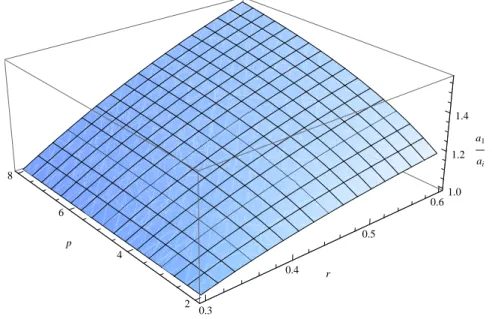
and/or as the number of predictors increase. Figure 1 plots the ratioa∗1
a∗
i
as a function ofpandrfor a fixed value ofr′ =.30. As expected, the relative weight placed on the first predictor increases smoothly as a function of bothpandr.
As an example, letp= 5, r=.6, r′=.25. This gives the following matrix for six predictors.
RXX =
x1 x2 x3 x4 x5 x6
x1 1 .6 .6 .6 .6 .6
x2 .6 1 .25 .25 .25 .25
x3 .6 .25 1 .25 .25 .25
x4 .6 .25 .25 1 .25 .25
x5 .6 .25 .25 .25 1 .25
x6 .6 .25 .25 .25 .25 1
RXXhas the following mini-max choice ofa,
a∗= [.57 .37 .37 .37 .37 .37].
In this example, the first element in the mini-max choice of weighting scheme, a∗
1, is over one and half
times as large as the remaining weights. This overweight-ing effect becomes even more pronounced when the pre-dictors in thisp-element array are mutually uncorrelated.
3.2
The case of mutually uncorrelated
pre-dictors
In contrast to the conditions identified in Hogarth and Karelaia (2005) and Fasolo et al. (2007), this
over-2Bothrandr′are required to be non-negative (as described in
Con-dition 1). Once one or both of these correlations becomes negative the eigenvalue described above,λmax, is no longer maximal. See
Figure 1: This figure displays the ratio a∗1
a∗
i
as a function ofrandpunder Condition 1 withr′=.3.
0.3
0.4
0.5
0.6
r
2 4
6 8
p
1.0 1.2
1.4
a1
ai
weighting effect becomes more pronounced as both the number of predictors increase and the inter-correlations of thep-many predictor array approach 0. In this section, we analyze the extreme case of a single cue positively correlated with p-many predictors which are mutually uncorrelated. This is a special case of Result 2 when
r′ = 0. In the asymptotic case, where the number of predictors is unbounded, the weights on the p-many predictors become arbitrarily small.
CONDITION2. Let RXX be defined as in Condition 1 and assumer′ = 0.
Condition 2 is a special case of Condition 1 so, ap-plying Result 1, the maximal eigenvalue ofRXXunder Condition 2 is equal to
λmax= 1 +r√p,
and the corresponding normed eigenvector (and the mini-max choice ofa) equals
a∗= [√1
2 1
√
2p
1
√
2p
1
√
2p
1
√
2p . . .
1
√
2p]. (7)
It is easy to see that as the number of predictors increases, i.e., as p becomes large, the weights on the
p-many predictor cue entries come arbitrarily close to 0 while a∗
1 remains constant. Put another way, when
r′ = 0, it is mini-max with respect to risk for a decision maker to heavily weight the single predictor. The effec-tiveness of this strategy becomes more pronounced as
the number of mutually uncorrelated predictors increases.
As a numerical example, letp= 5, r′ = 0. This gives the following matrix for six predictors.
RXX=
x1 x2 x3 x4 x5 x6
x1 1 r r r r r
x2 r 1 0 0 0 0
x3 r 0 1 0 0 0
x4 r 0 0 1 0 0
x5 r 0 0 0 1 0
x6 r 0 0 0 0 1
RXXhas the following mini-max choice ofa,
a∗= [.71 .32 .32 .32 .32 .32].
For this example, the weight onx1is more than double
the weight of each of the other predictors. In general, the ratio, a∗1
a∗
i =
√p. Thus, if for example, p = 100, the
weight onx1 would be 10 times as large as the weight
on any other predictor. We emphasize that the mini-max choice of weighting under Condition 2 does not depend upon the valuer.
dominates the inter-correlations of the remaining predic-tors. In the next section we demonstrate how this over-weighting effect applies to the performance of the Recog-nition Heuristic, showing that under Condition 2 a DM using only recognition will perform as well as a DM us-ing only knowledge.
4
The Recognition Heuristic
The RH is arguably the simplest of the “fast and frugal” heuristics that make up the “adaptive cognitive toolbox” (e.g., Gigerenzer et al., 1999). Quite simply, if a DM is choosing between two alternatives based on a target criterion, the recognized alternative is selected over the one that is not. Goldstein and Gigerenzer (2002) state that a “less-is-more effect” will be encountered whenever the probability of a correct response using only recogni-tion is greater than the probability of a correct response using knowledge (equations (1) and (2) in Goldstein & Gigerenzer, 2002), in their words: “whenever the ac-curacy of mere recognition is greater than the acac-curacy achievable when both objects are recognized.” Goldstein and Gigerenzer’s conditions for the success of the recog-nition heuristic depend upon the recogrecog-nition validity, i.e., the correlation between the target criterion and recogni-tion, which is assumed not to be directly accessible to the DM. Other environmental variables, called mediator vari-ables, which are positively correlated with both the target criterion (the ecological correlation) and the probability of recognition (the surrogate correlation), influence the DM as proxies for the target criterion. We build upon the recognition heuristic theory by defining a condition on the predictor cues that leads to a mini-max strategy closely mirroring the recognition heuristic. Conditions 1 and 2 depend only upon observable predictor cue inter-correlations and do not require the estimation or assump-tion of either a recogniassump-tion validity or corresponding sur-rogate and ecological correlations.
4.1
The Recognition Heuristic within a
lin-ear models framework
In this section we present a linear interpretation of the recognition heuristic by defining weighting schemes rep-resenting a DM using only recognition or only knowl-edge. We present a proof (Result 3) that a DM using only recognition will incur precisely the same amount of max-imal risk as a DM using only knowledge under Condition 2. This result states that a DM using only recognition will do at least as well as using only knowledge with respect to maximal risk. We compare these weighting schemes to each other, the optimal mini-max weighting, and Ordi-nary Least Squares (OLS).
To apply the optimality results presented above, we must first re-cast the RH within the linear model. Let
xi1 be the recognition response variable with respect to
the RH theory. Let the remainingp-many predictors cor-respond to an array of predictors relevant to the criterion under consideration. Within the RH framework, we shall refer to thesep-many variables as knowledge variables. This gives the following model,
Yi= β1xi1
| {z } recognition
+ p+1
X
j=2
βjxij
| {z } knowledge
+ ǫi
|{z} random error
. (8)
The recognition variable,xi1, is typically
conceptual-ized as a binary variable (e.g., Goldstein & Gigerenzer, 2002). Pleskac (2007) presents an analysis of the recog-nition heuristic in which recogrecog-nition is modeled as a con-tinuous variable integrated into a signal detection frame-work (see also Schooler and Hertwig, 2005). Note that our general result on maximal risk (5) holds for an arbi-trary matrix, X, in which predictor cues can be binary, continuous or any combination of the two types.
We use maximal risk as the principal measure of per-formance within the linear model, in contrast to previ-ous studies that used percentage correct within a two-alternative forced choice framework as a measure of model performance (e.g., Goldstein & Gigerenzer, 2002; Hogarth & Karelaia, 2005). As such, we do not compare individual values ofY for different choice alternatives. We instead make the assumption that a DM using “true”
βas a weighting scheme will outperform a DM using any other choice of weighting scheme. In our framework, minimizing maximal risk corresponds to a DM using a fixed weighting scheme that is “closer” to the “true”β
compared to any other fixed weighting scheme.
The Recognition Heuristic assumes that the DM can find him/herself in one of three mutually exclusive cases, that induce different response strategies: 1) neither alter-native is recognized and one must be selected at random, 2) both alternatives are recognized and only knowledge can be applied to choose one of them, and 3) only one alternative is recognized (the other is not), so the DM selects the alternative that is recognized. To model this process, we consider the following two choices of the weighting vectora:
• Only Recognition: let the first entry ofaRbe valued at one, all other entries are zero,
• Only Knowledge: let the first entry ofaKbe valued at zero, all other entries are one,
is modeled byaR, i.e., recognizing one choice alterna-tive without applying knowledge to the decision. The act of only using knowledge to select between items is modeled byaK, corresponding to a DM recognizing both choice alternatives and relying exclusively on knowledge to make the decision. We do not analyze the trivial case of neither alternative being recognized. To facilitate com-parison of these weights, letaMbe the mini-max weight-ing scheme from Result 1 and letOLS be the ordinary least squares estimate.
We can now describe and analyze when “less” infor-mation will lead to better performance in the language
of the linear model. When will aR perform as well
as, or better, than aK? Consider Condition 2, i.e., the case when the p-many predictor cues are mutually independent, r′ = 0. Under these circumstances the over-weighting effect of the mini-max vector is most pronounced and, surprisingly, the weighting schemesaR andaKincur exactly the same amount of maximal risk.
RESULT3. LetRXX be defined as in Condition 2, i.e.,
r′ = 0. Let aR andaK be defined as above. Then
maxRisk(aR) = maxRisk(aK).
PROOF. The proof follows by direct calculation using (5),
maxRisk(βˆaR) =kβk
2
a′
R(X′X) 2
aRa′RaR
(a′RX′XaR)2
+ a′RaRσ
2
a′
RX′XaR
=kβk2(pr2+ 1) +σ2
=kβk2
a′
K(X′X) 2
aKa′KaK
(a′
KX′XaK) 2
+ a′KaKσ2 a′
KX′XaK
= maxRisk(βˆaK).
Result 3 provides a new perspective on the phe-nomenon of “less” information leading to better perfor-mance: A simple single-variable decision heuristic (e.g., the recognition heuristic) is at least as good in terms of risk as equally weighting the remaining cues, e.g., knowl-edge.
We can directly compare the performance of
aK,aR,aM, and OLS by placing some weak
as-sumptions on the intercorrelation matrix of the predictors and the values of σ2 and kβk. First, we can bound
kβk2 by applying the inequalitykβk2 ≤ R2
λmin, where
R2 is the coefficient of multiple determination of the
linear model andλmin is the smallest eigenvalue of the
matrix RXX. Now, assuming values of σ2, R2, and a
structure ofRXX we can compare the maximal risk for
different weighting vectors as a function of sample size. Under our framework, sample size does not play a role in determining the mini-max choice of fixed weighting scheme, however we must consider sample size when comparing values of risk to other estimators, in this case OLS.
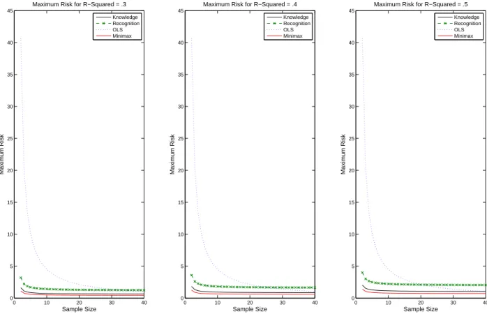
How do recognition and knowledge compare with the mini-max choice of weighting scheme? Figure 2 displays the maximal risk foraK,aR,aM, and OLS, under Con-dition 1 forp= 6, r=.6, r′ =.25, andσ2 = 2. The
three panels of Figure 2 corresponds toR2 =.3, .4, and
.5.
The performance of the knowledge, recognition, and mini-max weighting are comparable in all three condi-tions with the knowledge weighting,aK, coming closest to the optimal weighting scheme. In the case of Condition 1, recognition does not win out over knowledge, however recognition wins out over OLS for sample sizes as large asn= 30in the case ofR2=.3andn= 20for the case
ofR2=.5.
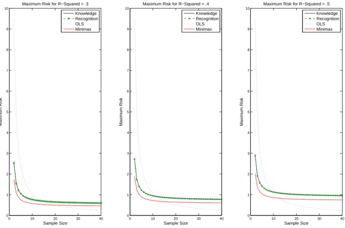
Figure 3 displays a corresponding set of graphs under Condition 2 forp= 3, r=.3, r′ = 0, andσ2 = 2. As
predicted by Result 3, recognition and knowledge have precisely the same maximal risk. The mini-max weight-ing scheme is quite comparable to knowledge/recognition performance. The performance of OLS improves in Con-dition 2; this follows from the matrixX′Xhaving fewer inter-correlated predictors.
To summarize, under Condition 1, both recognition and knowledge compare favorably to OLS and to the mini-max choice of weighting. Here recognition does not perform as well as knowledge but is comparable. Under Condition 2, the maximal risk of recognition and knowl-edge are identical, as shown in Result 3, and closely resemble the performance of the mini-max choice of weighting vector. In all cases, the performance of the dif-ferent weighting schemes are affected by the amount of variance in the error termǫi, in agreement with Hogarth
and Karelaia (2005).
4.2
Empirical example
Figure 2: This figure displays the maximal risk as a function of sample size for four choices of weighting schemes: aR(solely recognition),aK(solely knowledge),aM(mini-max weighting), andOLS(ordinary least squares). These values are displayed under Condition 1, wherer′ =.25, r = .6, p = 6,andσ2 = 2. The left-hand graph displays
these values assumingR2 = .3. The center and right-hand graphs display these values forR2 = .4andR2 = .5
respectively.
0 10 20 30 40
0 5 10 15 20 25 30 35 40 45
Maximum Risk for R−Squared = .3
Sample Size
Maximum Risk
0 10 20 30 40
0 5 10 15 20 25 30 35 40 45
Maximum Risk for R−Squared = .4
Sample Size
Maximum Risk
0 10 20 30 40
0 5 10 15 20 25 30 35 40 45
Maximum Risk for R−Squared = .5
Sample Size
Maximum Risk
Knowledge Recognition OLS Minimax
Knowledge Recognition OLS Minimax
Knowledge Recognition OLS Minimax
based on their names alone. Each city was assigned a recognition score based on the number of subjects (out of a possible 25) who recognized it. In addition, we have nine binary attributes for each city that serve as predic-tors — see Table 1 for a description of the predictor cues (Gigerenzer et al., 1999). The inter-correlation matrix of the 10 predictors is presented in Table 2.
The data in Table 2 strongly resemble the optimality conditions described in Conditions 1 and 2. Recogni-tion is significantly and positively correlated with 7 of the 9 predictor cue variables atp < .01. Twenty four of (9×8/2 =) 36 cue inter-correlations are not significantly greater than 0, which strongly resembles Condition 2. Each of the nine predictors in the array (x2, x3, . . . , x10)
has its highest correlation with recognition with one or two exceptions in each column, i.e., r1j > rkj,∀k ∈
{2,3, . . . ,10}holds for 7 of the 9 predictors with at most one exception each. The average correlation of the recog-nition variable with the other nine cue predictors is .29 and the average inter-correlation of the 9 predictors is .11.
To summarize, these data are consistent with the
struc-ture of Conditions 1 and 2. The nine predictor cues for the cities appear to contribute “unique” pieces of information to the linear model (8), yet most of these predictors have large positive correlations with recognition. We conclude that in the case of the “German Cities” stimuli, it is an optimal mini-max strategy to “overweight” recognition.
5
Discussion
(Gold-Figure 3: This figure displays the maximal risk as a function of sample size for four choices of weighting schemes: aR(solely recognition),aK(solely knowledge),aM(mini-max weighting), andOLS(ordinary least squares). These values are displayed under Condition 2, wherer′ = 0, r = .3, p = 3,andσ2 = 2. The left-hand graph displays
these values assumingR2 = .3. The center and right-hand graphs display these values forR2 = .4andR2 = .5
respectively.
0 10 20 30 40
0 1 2 3 4 5 6 7 8 9 10
Sample Size
Maximum Risk
Maximum Risk for R−Squared = .3
0 10 20 30 40
0 1 2 3 4 5 6 7 8 9 10
Sample Size
Maximum Risk
Maximum Risk for R−Squared = .4
0 10 20 30 40
0 1 2 3 4 5 6 7 8 9 10
Sample Size
Maximum Risk
Maximum Risk for R−Squared = .5
Knowledge Recognition OLS Minimax
Knowledge Recognition OLS Minimax
Knowledge Recognition OLS Minimax
stein & Gigerenzer, 2002) — and provided a condition where a DM using solely recognition to choose between two choice alternatives would incur precisely the same maximal risk as a decision maker using only knowledge (Result 3). We illustrated these results by analyzing the inter-cue correlation matrix from an experiment using the well-known “German Cities” stimuli. This dataset pro-vides empirical support for the descriptive accuracy of Conditions 1 and 2, and therefore for the over-weighting of a single predictor cue.
The performance of single-variable decision heuristics like the RH depends upon the complex interplay of a DM’s cognitive capacities and the structure of the envi-ronment, i.e., the relationships among predictor cues and the criterion variable. When all predictor cues are highly positively correlated we have conditions for a “flat max-imum effect”; here a single-variable decision rule will do as well as any other simple weighting rule. In other words, any choice of weighting scheme utilizes, essen-tially, the same information in the environment. The DM benefits in such “single-factor” environments as he can
use a less cognitively demanding strategy and not suf-fer any serious penalties for doing so. In such single-factor environments the optimal weighting scheme may not resemble a single-variable rule, but the differences in performance are so small that it doesn’t really mat-ter. The DM is “rational” because he/she is balancing cognitive effort with the demands of the environment, the “twin-blades” of Simon’s scissors (Simon, 1990) or seek-ing to optimize the accuracy / effort tradeoff (Payne et al., 1993).
Table 1: Predictor Cues for the “German Cities” Study (Gigerenzer et al., 1999; Goldstein, 1997).
Cue description Predictor Cue
Recognition x1
National capital (Is the city the national capital?) x2
Exposition Site (Was the city once an exposition site?) x3
Soccer team (Does the city have a team in the major leagues?) x4
Intercity train (Is the city on the Intercity line?) x5
State capital (Is the city a state capital?) x6
License plate (Is the abbreviation only one letter long?) x7
University (Is the city home to a university?) x8
Industrial belt (Is the city in the industrial belt?) x9
East Germany (Was the city formerly in East Germany?) x10
Table 2: Inter-correlation Matrix of Predictor Cues for “German Cities” Study (Goldstein, 1997). The variables are labeled as in Table 1. Values denoted with∗are significant atp < .05, values with+atp < .01, wherepdenotes the
standard p-value.
x1 x2 x3 x4 x5 x6 x7 x8 x9 x10
x1 1 .30+ .39+ −.04 −.23∗ .47+ .36+ .64+ .28+ .46+
x2 .30+ 1 .19 −.12 .02 .13 .13 .45+ −.05 .20
x3 .39+ .19 1 .14 −.22∗ .21 .27∗ .37+ .24∗ .14
x4 −.04 −.12 .14 1 −.20 .26∗ .02 −.11 −.05 −.25∗
x5 −.23∗ .02 −.22∗ −.20 1 −.10 −.09 −.05 −.05 −.17
x6 .47+ .13 .21 .26∗ −.10 1 .17 .54+ .21 .27∗
x7 .36+ .13 .27∗ .02 −.09 .17 1 .19 .06 .49+
x8 .64+ .45+ .37+ −.11 −.05 .54+ .19 1 .25∗ .37+
x9 .28+ −.05 .24∗ −.05 −.05 .21 .06 .25∗ 1 .11
x10 .46+ .20 .14 −.25∗ −.17 .27∗ .49+ .37+ .11 1
cognitively demanding and one that resembles an opti-mal strategy in terms of minimizing risk.
To clarify, we are not proposing a decision heuristic, e.g., pick the most highly correlated predictor cue, but point out that in certain decision environments single-variable heuristics are almost optimal. Our definition of risk, a common benchmark in the statistical literature, may help explain why our “favorable” conditions for a single-variable rule differ from previous ones. Minimiz-ing maximal risk is equivalent to choosMinimiz-ing a weightMinimiz-ing scheme that is, on average, closest to the true state of the nature,β. This definition accounts for an infinity of pos-sible relationships between the predictor cues and the cri-terion variable, focusing on the conditions that yield the least favorable relationships. By this measure, it is better to over-weight a single variable that contains some
infor-mation about all of the predictor cues than to weight, say equally, all of the predictor cues taking the chance that some combination of them may not be at all predictive of the criterion. In this way, we account for an infinity of possible validity structures, even though our formulation does not require any specific assumptions on the validi-ties themselves.
et al, 1999). We do assume in our analysis that the deci-sion maker always utilizes the single predictor that con-forms to our sufficient conditions. We do not assume any other structure to predictor cue selection or application. Thus, recognition is a natural application of these results, as the Recognition Heuristic does not presuppose a pre-dictor cue selection process.
Our results easily extend to recent generalizations of the RH. Several studies have extended the application of the RH beyond simple 2-alternative forced choice ton -alternative forced choice (Beaman, McCloy, & Smith, 2006; Frosch, Beaman, & McCloy, 2007; McCloy & Beaman, 2004; McCloy, Beaman, & Goddard, 2006); see also Marewski, Gaissmaier, Schooler, Goldstein, & Gigerenzer (2010) for a related framework employing “consideration sets”. Our linear modeling framework does not depend upon the number of choice alternatives being considered. Our only assumption is that the DM differentially selects alternatives based on the value of the criterion as implied by his/her choice of predictor cue weights. Thus, moving from 2 to nalternatives under consideration does not change our key results, a DM uti-lizing our optimal weighting scheme to select among a set of alternatives will “on average” perform better than another DM using a sub-optimal weighting scheme. Our framework also allows the predictors to be either binary or continuous or any combination thereof. In this way, our results easily extend to continuous representations of recognition. Several authors have previously explored continuous representations of recognition within the con-texts of both signal detection models (Pleskac, 2007) and the ACT-R framework (Schooler & Hertwig, 2005).
Although we applied our model successfully in the context of RH, we must remain silent on the psycholog-ical nature of some key concepts underlying the theory in this domain. For example, we treat thisp-many pre-dictor cue “knowledge” array as an abstract quantity and subsequently do not place any special psychological re-strictions or assumptions upon these predictor cues. We also recognize that there is an ongoing debate in the lit-erature as to the interplay between knowledge, learning, and memory with regard to recognition and that there are many factors that influence whether DMs’ choices are consistent with the RH (e.g., Newell & Fernandez, 2006; Pachur, Bröder, & Marewski, 2008; Pachur & Hertwig, 2006). However, our model is mute with respect to these debates.
The results we have presented are general, and while we have restricted their application to the study of recog-nition, they could be applied to other domains. For ex-ample, in a well-publicized study on heart disease, Batty, Deary, Benzeval, and Der (2010) found that IQ was a bet-ter predictor of heart disease than many other, more tra-ditional, predictors such as: income, blood pressure, and
low physical activity. One possible explanation of their findings is that, historically, IQ tends to correlate to some degree with each of the remaining predictors (e.g., Batty, Deary, Schoon, & Gale, 2007; Ceci & Williams, 1997; Knecht et al., 2008). In light of the results presented in our paper, it is perhaps not so surprising that IQ is a “ro-bust” predictor of heart disease.
Our results do not imply that ordinary least squares or other statistical/machine-learning weighting processes are “sub-optimal.” Given an infinite amount of data, weighting schemes derived from such processes would indeed be optimal with respect to almost any measure. Our results apply to fixed weighting schemes, which, in the context of small sample sizes tend to perform very well as they do not “over-fit” the observed data. In other words, fixed weighting schemes cross-validate extremely well compared to other, more computationally intensive, estimation procedures for situations involving small sam-ple sizes and/or large variances in the error terms.
Gigerenezer et al., (1996; 1999) argue that “fast and frugal” heuristics are a rational response to the “bounded” or “finite” computational mind of a decision maker. This article raises many new questions regarding the rational-ity of simple decision heuristics. Given infinite compu-tational might and a relatively small sample of data, a “Laplacean Demon’s” choice of weighting scheme might resemble that of a “fast and frugal” decision maker. In other words, DMs could be reasoning like a “Laplacean Demon” would if the demon were given limited infor-mation, but retained the assumption of infinite computa-tional ability.
References
Batty, G. D., Deary, I. J., Benzeval, M., & Der, G. (2010). Does IQ predict cardiovascular disease mortality as strongly as established risk factors? Comparison of effect estimates using the West of Scotland Twenty-07 cohort study. European Journal of Cardiovascular Prevention and Rehabilitation, 17, 24–27.
Batty, G. D., Deary, I. J., Schoon, I., & Gale, C. R. (2007). Childhood mental ability in relation to food intake and physical activity in adulthood: The 1970 British cohort study. Pediatrics, 119, 38–45.
Baucells, M., Carrasco, J. A., & Hogarth, R. M. (2008). Cumulative dominance and heuristic performance in binary multiattribute choice. Operations Research, 56, 1289–1304.
Lawrence Erlbaum Associates.
Bröder, A. (2000). Assessing the empirical validity of the “take-the-best” heuristic as a model of human proba-bilistic inference. Journal of Experimental Psychol-ogy: Learning, Memory, and Cognition, 26, 1332– 1346.
Bröder, A., & Schiffer, S. (2003). Take the best ver-sus simultaneous feature matching: Probabilistic infer-ences from memory and effects of representation for-mat. Journal of Experimental Psychology: General, 132, 277–293.
Brunswik, E. (1952). The conceptual framework of psy-chology. Chicago: The University of Chicago Press. Ceci, S. J., & Williams, W. M. (1997). Schooling,
intelli-gence, and income. American Psychologist, 52, 1051– 1058.
Davis-Stober, C. P., Dana, J., & Budescu, D. V. (2010) A constrained linear estimator for multiple regression. Psychometrika, in press.
Dawes, R. M. (1979). The robust beauty of improper lin-ear models. The American Psychologist, 34, 571–582. Dawes, R. M., & Corrigan, B. (1974). Linear models in decision making. Psychological Bulletin, 81, 95–106. Einhorn, H. J., & Hogarth, R. M. (1975). Unit weighting
schemes for decision making. Organizational Behav-ior and Human Performance, 13, 171–192.
Fasolo, B., McClelland, G. H., & Todd, P. M. (2007). Escaping the tyranny of choice: When fewer attributes make choice easier. Marketing Theory, 7, 13–26. Frosch, C. A., Beaman, C. P., & McCloy, R. (2007). A
little learning is a dangerous thing: An experimen-tal demonstration of ignorance-driven inference. The Quarterly Journal of Experimental Psychology, 60, 1329–1336.
Gigerenzer, G., & Goldstein, D. G. (1996). Reasoning the fast and frugal way: Models of bounded rationality. Psychological Review, 103, 650–669.
Gigerenzer, G., Todd, P. M. & the ABC Research Group. (1999). Simple heuristics that make us smart. New York: Oxford university Press.
Goldstein, D. G. (1997). Models of bounded rational-ity for inference. Doctoral thesis, The Universrational-ity of Chicago. Dissertation Abstracts International, 58(01), 435B. (University Microfilms No. AAT 9720040). Goldstein, D. G., & Gigerenzer, G. (2002). Models of
ecological rationality: The recognition heuristic. Psy-chological Review, 109, 75–90.
Hammond, K. R., Hursch, C. J., & Todd, F. J. (1964). Analyzing the components of clinical inference. Psy-chological Review, 71, 438–456.
Hertwig, R., & Todd, P. M. (2003). More is not always better: The benefits of cognitive limits. In D. Hardman, & L. Macchi (Eds.), Thinking: Psychological
perspec-tives on reasoning, judgment and decision making (pp. 213–231). Chichester, England: Wiley.
Hogarth, R. M., & Karelaia, N. (2005). Ignoring informa-tion in binary choice with continuous variables: When is less “more”? Journal of Mathematical Psychology, 49, 115–124.
Hogarth, R. M., & Karelaia, N. (2006). “Take-The-Best” and other simple strategies: Why and when they work “well” with binary cues. Theory and Decision, 61, 205–249.
Katsikopoulos, K. V., & Martignon, L. (2006). Naïve heuristics for paired comparisons: Some results on their relative accuracy. Journal of Mathematical Psy-chology, 50, 488–494.
Keeney, R. L., & Raiffa, H. (1993). Decisions with multi-ple objectives: Preferences and value tradeoffs. Cam-bridge: Cambridge University Press.
Knecht, S., Wersching, H., Lohmann, H., Bruchmann, M., Duning, T., Dziewas, R., Berger, K., & Ringel-stein, E. B. (2008). High-normal blood pressure is as-sociated with poor cognitive performance. Hyperten-sion, 51, 663–668.
Marewski, J. N., Gaissmaier, W., Schooler, L. J., Gold-stein, D. G., & Gigerenzer, G. (2010). From recogni-tion to decisions: Extending and testing recognirecogni-tion- recognition-based models for multi-alternative inference. Psycho-nomic Bulletin & Review, 17, 287–309.
Martignon, L., & Hoffrage, U. (1999). Why does one-reason decision making work? A case study in eco-logical rationality. In G. Gigerenzer, P. M. Todd, & the ABC Research Group (Eds.), Simple heuristics that make us smart (pp. 119–140). New York: Oxford Uni-versity Press.
Martignon, L., & Hoffrage, U. (2002). Fast, frugal, and fit: Simple heuristics for paired comparison. Theory and Decision, 52, 29–71.
McCloy, R., & Beaman, C. P. (2004). The recognition heuristic: Fast and frugal but not as simple as it seems. In K. Forbus, D. Gentner, & T. Regier (Eds.), Pro-ceedings of the Twenty-Sixth Annual Conference of the Cognitive Science Society (pp. 933–937). Mahwah, NJ: Lawrence Erlbaum Associates.
McCloy, R., Beaman, C. P., & Goddard, K. (2006). Rich and famous: Recognition-based judgment in the Sun-day Times rich list. In R. Sun & N. Miyake (Eds.), Pro-ceedings of the Twenty-Eighth Annual Conference of the Cognitive Science Society (pp. 1801–1805). Hills-dale, NJ: Lawrence Erlbaum Associates.
Newell, B. R., & Fernandez, D. (2006). On the binary quality of recognition and the inconsequentiality of further knowledge: Two critical tests of the recognition heuristic. Journal of Behavioral Decision Making, 19, 333–346.
look at the rest? Factors influencing “one-reason” de-cision making. Journal of Experimental Psychology: Learning, Memory, and Cognition, 29, 53–65. Pachur, T., & Biele, G. (2007). Forecasting from
igno-rance: The use and usefulness of recognition in lay predictions of sports events. Acta Psychologica, 125, 99–116.
Pachur, T., Bröder, A., & Marewski, J. N. (2008). The recognition heuristic in memory-based inference: Is recognition a non-compensatory cue? Journal of Be-havioral Decision Making, 21, 183–210.
Pachur, T., & Hertwig, R. (2006). On the psychology of the recognition heuristic: Retrieval primacy as a key determinant of its use. Journal of Experimental Psy-chology, 32, 983–1002.
Payne, J. W., Bettman, J. R., & Johnson, E. J. (1993). The adaptive decision maker. New York: Cambridge University Press.
Pleskac, T. J. (2007). A signal detection analysis of the recognition heuristic. Psychonomic Bulletin & Review, 14, 379–391.
Scheibehenne, B., & Bröder, A. (2007). Predicting Wim-bledon 2005 tennis results by mere player name recog-nition. International Journal of Forecasting, 23, 415– 426.
Schooler, L. J., & Hertwig, R. (2005). How forgetting aids heuristic inference. Psychological Review, 112, 610–628.
Serwe, S., & Frings, C. (2006). Who will win Wim-bledon? The recognition heuristic in predicting sports events. Journal of Behavioral Decision Making, 19, 321–332.
Shanteau, J., & Thomas, R. P. (2000). Fast and frugal heuristics: What about unfriendly environments? Be-havioral and Brain Sciences, 23, 762–763.
Simon, H. A. (1990). Invariants of human behavior. An-nual Review of Psychology, 41, 1–19.
Snook, B., & Cullen, R. M. (2006). Recognizing na-tional hockey league greatness with an ignorance-based heuristic. Canadian Journal of Experimental Psychology, 60, 33–43.
Todd, P. M. (1999). Simple inference heuristics versus complex decision machines. Minds and Machines, 9, 461–477.