www.atmos-chem-phys.org/acp/3/697/
Chemistry
and Physics
Detailed modeling of mountain wave PSCs
S. Fueglistaler1, S. Buss1, B. P. Luo1, H. Wernli1, H. Flentje2, C. A. Hostetler3, L. R. Poole3, K. S. Carslaw4, and Th. Peter1
1Atmospheric and Climate Science, ETH Z¨urich, Switzerland 2DLR Oberpfaffenhofen, 82230 Wessling, Germany
3NASA Langley Research Center, Hampton, VA, USA 4School of the Environment, Univ. of Leeds, Leeds, UK
Received: 6 November 2002 – Published in Atmos. Chem. Phys. Discuss.: 13 January 2003 Revised: 3 June 2003 – Accepted: 4 June 2003 – Published: 11 June 2003
Abstract. Polar stratospheric clouds (PSCs) play a key role in polar ozone depletion. In the Arctic, PSCs can oc-cur on the mesoscale due to orographically induced grav-ity waves. Here we present a detailed study of a moun-tain wave PSC event on 25–27 January 2000 over Scan-dinavia. The mountain wave PSCs were intensively ob-served by in-situ and remote-sensing techniques during the second phase of the SOLVE/THESEO-2000 Arctic cam-paign. We use these excellent data of PSC observations on 3 successive days to analyze the PSCs and to perform a detailed comparison with modeled clouds. We simu-lated the 3-dimensional PSC structure on all 3 days with a mesoscale numerical weather prediction (NWP) model and a microphysical box model (using best available nucleation rates for ice and nitric acid trihydrate particles). We show that the combined mesoscale/microphysical model is capa-ble of reproducing the PSC measurements within the uncer-tainty of data interpretation with respect to spatial dimen-sions, temporal development and microphysical properties, without manipulating temperatures or using other tuning pa-rameters. In contrast, microphysical modeling based upon coarser scale global NWP data, e.g. current ECMWF anal-ysis data, cannot reproduce observations, in particular the occurrence of ice and nitric acid trihydrate clouds. Com-bined mesoscale/microphysical modeling may be used for detailed a posteriori PSC analysis and for future Arctic cam-paign flight and mission planning. The fact that remote sens-ing alone cannot further constrain model results due to un-certainities in the interpretation of measurements, underlines the need for synchronous in-situ PSC observations in cam-paigns.
Correspondence to:S. Fueglistaler ([email protected])
1 Introduction
Polar stratospheric clouds (PSCs) play a key role in po-lar ozone depletion. On the aerosol surface, heterogeneous chemical reactions take place that activate chlorine from in-ert reservoir species (ClONO2, HCl) to Cl2, which is rapidly photolyzed into atomic chlorine radicals (Solomon et al., 1986; Tolbert et al., 1987):
ClONO2+HCl−→Cl2+HNO3 (1)
and
HCl+HOCl−→Cl2+H2O (2)
Cl2+hν−→Cl+Cl (3)
The chlorine radicals then destroy ozone in catalytic cycles (Molina and Molina , 1987; McElroy et al., 1986).
In addition, PSCs can permanently remove HNO3through sedimentation, a process termed denitrification, which slows the transfer of active chlorine into CLONO2and hence fur-ther promotes ozone destruction (WMO, 1999; Waibel et al., 1999; Tabazadeh et al., 2000; Gao et al., 2001).
the air in the polar vortex, despite their relatively small spa-tial dimension (Carslaw et al., 1998b).
Based on lidar observations by Browell et al. (1990), Toon et al. (1990) identified three distinct types of PSCs. Type 1a and 1b both show low to moderate backscatter ratios (BSR). In contrast to type 1b which was later identified as super-cooled ternary (HNO3/H2SO4/H2O) solution (STS) droplets with number densities ∼ 10 cm−3 (Carslaw et al., 1994), type 1a shows moderate aerosol depolarization (δaerosol), which Biele et al. (2001) interpreted as containing small number densities (n . 10−2cm−3) of aspherical particles, most likely nitric acid trihydrate (NAT). Type 2 PSCs show high BSRs and moderate to high depolarisation, attributed to water ice particles. Later, Tsias et al. (1999) identified type 1a-enh PSCs as similar to type 1a but with enhanced NAT particle number densities (n & 0.1 cm−3). First evidence from in-situ measurements for the presence of NAT particles in PSCs was given by Voigt et al. (2000) from a balloon-borne experiment during the SOLVE/THESEO-2000 cam-paign. During the same campaign, Fahey et al. (2001) de-tected for the first time very large HNO3-containing (presum-ably NAT) particles in very low number densities (so-called “NAT-rocks”) which can efficiently denitrify the polar strato-sphere. Apart from ternary solution droplets and NAT the existence of other HNO3containing hydrates, such as nitric acid dihydrate (NAD), is also still under debate.
Carslaw et al. (1998a) and Wirth et al. (1999) success-fully modeled lidar measurements of mountain wave PSCs from flights that were parallel to the wind direction (so-called quasi-Lagrangian measurements). They used a microphysi-cal box model that microphysi-calculated the PSC microphysics along a manually inferred trajectory, and without exact knowledge of ice or NAT nucleation rates. Using T-Matrix calcula-tions for aspherical solid particles (Mishchenko , 1991) and Mie calculations with an index of refraction as a function of aerosol composition, temperature and wavelength for the liq-uid aerosol (Krieger et al., 2000), it was shown that the sim-ulated lidar signal inferred from the modeled microphysics could be brought into good agreement with the observations, provided that the trajectory was chosen carefully and that the number densities of ice and NAT particles were chosen within plausible limits.
2 Mesoscale/microphysical modeling approach
Here we significantly improve the method of Carslaw et al. (1998a) and Wirth et al. (1999) and extend its scope. In-stead of manually inferred trajectories we use trajectories from mesoscale numerical weather prediction (NWP) mod-els. This greatly reduces the degrees of freedom of the model. Trajectories from NWP models furthermore allow us to simulate the 3-dimensional structure of PSCs, and al-low predictions of PSC occurrences where no measurements are available. We use trajectories from the mesoscale High
GM
50
50 50
50 50
50
50
60
60
GM
50
50
50
50
50
50
50
50
60
60
60
60
60
70
GM
50
50
50
50
50
50 50
60 60
60
70 70 80
✁
✁✄✂☎
✁
✁
✆
✁✄✂☎
✆✝✂☎
✁
✁✄✂☎
✁ ✆
☎
✞✠✟☛✡✌☞
✂
✟
✍✏✎✒✑✔✓✝✕✝✖✗✕✙✘
✍
✎✛✚✜✓✣✢
✍✏✎✒✑✔✓✝✕✝✖✗✕✙✘
✍✏✎✤✚✥✓
✍✧✦✕ ✦✎★✘ ☞ ✍ ✎✤✑✔✓★✕✄✖✙✕✗✘
✟
✍ ✎✛✚✜✓
✍☛✎✛✚✜✓
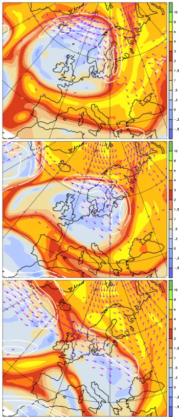
Fig. 1. The synoptic situation at 12:00 UTC, 25 January (top), 26
Resolution Model (HRM, cf. Sect. 3.5) and compare them with trajectories from ECMWF analysis data.
An updated version of the microphysical box model is used, which calculates the nucleation of ice and NAT parti-cles. We use the nucleation rates given by Koop et al. (2000) for the homogeneous freezing of ice particles and those pro-vided by Luo et al. (2002) for the NAT nucleation on ice sur-faces exposed to the gas phase, instead of adjusting the solid particle number densities manually as was done by Carslaw et al. (1998a) and Wirth et al. (1999). The approach cho-sen in this study uses the current understanding of numerical weather prediction models and microphysical processes in a self-consistent way without any “tuning”, such that the simu-lations can be run fully automatically. This enables to obtain the morphology of PSCs in 2-D or 3-D calculations instead of focusing on one or two selected trajectories. We compare the results of these simulations to measurements allowing to judge the accuracy of the state-of-the-art modeling.
The combined mesoscale/microphysical model is applied to the period 25–27 January over Scandinavia. The data ac-quired in this period during the SOLVE/THESEO-2000 Arc-tic campaign provide probably the most complete collection of data of a mountain wave PSC event. For all three succes-sive days the simulations were performed with exactly the same setup, showing the robustness of the approach.
3 Data and tools
3.1 Synoptic situation, 25–27 January 2000
The meteorological situation leading to the mountain wave PSCs on 25–27 January over Scandinavia was discussed by D¨ornbrack et al. (2002). Figure 1 shows the potential vor-ticity (PV) field on the 345 K isentropic surface, wind speed in the upper troposphere (250 hPa) and wind vectors in the lower troposphere (900 hPa) for 25–27 January 2000. The isentropic PV charts are well suited, for instance, to iden-tify large-scale upper-tropospheric anticyclones (character-ized by PV values < 2 pvu) and jet-stream regions (char-acterized by strong horizontal PV gradients).
In agreement with Doernbrack et al. we note for 25 Jan-uary the existence of an extreme upper-level anticyclone over the UK, Iceland and Norway with strong low-level winds to-wards northern Norway and a northerly upper tropospheric jet over Scandinavia. In the course of the 3 days the anticy-clone shifts southward and on 26 January a very strong jet is directly over central Scandinavia. The jet is almost par-allel to strong near surface westerlies, which provides very favourable conditions for excitation and vertical propagation of mountain waves. On 27 January the anticyclone shifted further south, leaving relatively weak low- and upper-level winds over Scandinavia, except for the southernmost part with upper-level wind speeds∼50 m/s.
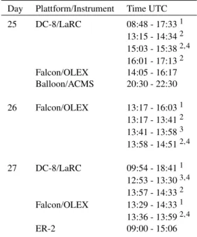
Table 1. Overview of platforms and instruments 25–27 January
2000.
1Total recording time;2flight crossing Scandinavian mountain;3
flight not aligned to wind direction;4lidar data shown in this study
Day Plattform/Instrument Time UTC
25 DC-8/LaRC 08:48 - 17:331
13:15 - 14:342 15:03 - 15:382,4 16:01 - 17:132
Falcon/OLEX 14:05 - 16:17
Balloon/ACMS 20:30 - 22:30
26 Falcon/OLEX 13:17 - 16:031
13:17 - 13:412 13:41 - 13:583 13:58 - 14:512,4
27 DC-8/LaRC 09:54 - 18:411
12:53 - 13:303,4 13:57 - 14:332
Falcon/OLEX 13:29 - 14:331
13:36 - 13:592,4
ER-2 09:00 - 15:06
3.2 PSC measurement
In this study lidar data is used from the NASA LaRC Aerosol Lidar (a piggy-back instrument to the NASA GSFC ARO-TEL lidar, 532 nm, 1064 nm) on board the NASA DC-8 air-craft and the DLR OLEX lidar system (354 nm, 532 nm, 1064 nm) on board the Falcon aircraft (Flentje et al., 1999). Both systems measure total backscatter at all wavelengths and depolarization at 532 nm, which allows discrimination of spherical (STS) and aspherical (e.g. NAT and ice) parti-cles. In addition, we will refer to the results of the balloon-borne measurements of 25 January (Voigt et al., 2000) and the in-situ measurements on board the stratospheric research aircraft ER-2 on 27 January (Northway et al., 2002). Table 1 provides an overview of the platforms in operation on 25– 27 January and from the data used in this study. The data is analyzed in Sect. 4.
3.3 Analysis of lidar data
A lidar system emits a laser pulse and measures the backscat-ter from aerosols and air molecules as a function of time. The backscatter ratio BSR is defined as
BSR=1+β
aerosol
βair , (4)
where βaerosol is the backscatter coefficient of aerosol and
180.0 182.5 182.5 185.0 185.0 185.0 185.0 187.5 187.5 187.5 187.5 190.0 190.0 190.0 190.0 190.0 195.0 195.0 195.0 195.0 195.0 195.0 200.0 200.0 200.0 200.0 200.0 205.0 205.0 205.0 205.0 215 215 215
225 225 225
235 235
235
245 245 245
255 255 255 265 265 265 3 8 13 18 23 28 longitude altitude [km]
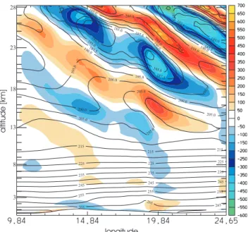
Fig. 2. West-east cross-section of HRM simulation, 15:00 UTC,
26 January 2000, along flight path of Falcon aircraft (leg 3, see Fig. 6). Color coded: horizontal divergence (blue) and convergence (red) of wind field [106s−1]. Black solid lines: temperature [K], lowermost line shows the orography.
coefficientβt ot al = βaerosol+βair, and in order to obtain the backscatter ratio, the backscatter coefficientβair has to be calculated as a function of air density. The depolarization of the scattered laser pulse yields information about the shape of the scatterer. The aerosol depolarization is defined as:
δaerosol=β
aerosol
⊥
βkaerosol (5)
whereβ⊥aerosolis the perpendicular aerosol backscatter coef-ficient andβkaerosolis the parallel aerosol backscatter coeffi-cient. The color ratio is defined as the ratio of the aerosol backscattering coefficient at two wavelengths λ1, λ2 with
λ1< λ2:
CR(λ1/λ2)=
βλaerosol
1
βλaerosol
2
(6) The color ratio is very sensitive to the size of the scat-terers, but independent of the number of scatterers. We will use the following notation: the backscatter ratio at 1064nm ≡ BSR(1064), the color ratio β532aerosol/β1064aerosol ≡ CR(532/1064), and the aerosol depolarization at 532nm≡
δaer(532).
Based on long term lidar observations over Ny Alesund, Spitsbergen (78.9◦N, 11.9◦E) and T-Matrix calculations, Biele et al. (2001) presented a classification of lidar data. They classify PSCs into the following types: type 1a (aspher-ical particles, most likely NAT, low particle number densi-tiesn≈10−2cm−3), type 1a-enh (aspherical particles, most
likely NAT, high particle number densitiesn & 0.1 cm−3), type 1b (ternary HNO3/H2SO4/H2O aerosol droplets (STS),
n≈ 10 cm−3), type mix (spherical and aspherical particles, likely NAT and STS particles mixed externally and not in thermodynamic equilibrium) and type 2 (ice particles,n =1-10 cm−3). We will use this classification as a reference in our lidar data interpretation.
The backscatter of aspherical particles may be calcu-lated using the T-Matrix method (Mishchenko , 1991) (with spheroids of aspect ratio 0.5-1.5 as proxies for ice and NAT particles). The index of refraction is 1.31 for ice and 1.48 for NAT (Middlebrook et al., 1994; Toon et al., 1994), that of STS obtained from Krieger et al. (2000).
3.4 Microphysical modeling
A microphysical box model is used to calculate the evolu-tion of the aerosol along a trajectory. The thermodynam-ics governing the condensation/evaporation kinetthermodynam-ics of water and nitric acid by the aqueous sulfuric acid aerosol is calcu-lated from an ion-interaction model (Pitzer , 1991; Luo et al., 1995; Meilinger et al., 1995). The aerosol size distribution is assumed to be log-normal with an initial mode radius of 0.06µm and a mode width of 1.6 atT =210 K. All calcula-tions were performed withn=13 cm−3background aerosol particles, the sensitvity of the model results on background aerosol number density being small. The size distribution is modeled using 26 size bins for the liquid aerosol. Ho-mogeneous ice nuleation in STS droplets is calculated from the nucleation rates by Koop et al. (2000), and the ice vapor pressure is calculated in accordance with Marti and Mauers-berger (1993). NAT nucleation on exposed ice surfaces is calculated in accordance with Luo et al. (2002), and the NAT vapor pressure is taken from Hanson and Mauersberger (1988). For each timestep, the number of nucleating ice and NAT particles is calculated for each size bin and transferred to new bins of their own. Upon evaporation of ice and NAT particles, the resulting droplets return into their original size bin.
The water mixing ratio in the Arctic stratosphere is taken from a linear interpolation of measured water mixing ratios on 27 January 2000 with a mixing ratioχH2O = 4.2 ppmv at 400 K andχH2O = 6.3 ppmv at 600 K (Schiller et al., 2002). In agreement with Arctic mid-winter measurements (Kleinb¨ohl et al., 2003), an HNO3profile with constant vol-ume mixing ratio of 7.5 ppmv is used (altitude-dependent deviations in the order of 30 % may be expected in a real profile, but do not significantly alter model results).
3.5 Mesoscale modeling
2001). Furthermore, D¨ornbrack et al. (2002) modeled 25– 27 January 2000 episode with the mesoscale MM5 model. Here we calculated a series of mesoscale simulations with the High Resolution Model (HRM) (Majewski et al., 1991). A former version of this limited-area model was used op-erationally by the German and Swiss Weather Services un-til early 2001 and is widely used in the hindcast mode for regional climate simulations (e.g. L¨uthi et al., 1996). The model integrates the set of primitive equations in the hydro-static limit. The initial and boundary conditions are taken from ECMWF analyses, and a radiative upper boundary con-dition prevents wave reflection. We use a dry physics version of the model without radiation and a horizontal resolution of 0.125◦ (corresponding to ∼14 km) and 60 vertical lev-els up to 4 hPa (regularly spaced in logp). Further details of the model setup can be found in Buss et al. (A gravity wave induced ice cloud over Greenland: Model validation and investigation of dynamical mechanisms, manuscript in preparation). Sensitivity studies showed that the simulation of the gravity wave and the associated temperature fields is sensitive to horizontal and vertical resolution and the initial-ization time, but insensitive to the height of the uppermost model level as well as inclusion of radiatation and moisture. For the simulations presented here, the orography was low-pass filtered with a conservative diffusion operator in order to eliminate the grid-scale components of the gravity wave. The simulations were started every 24 hours for integration peri-ods of 36 hours. The first 12 hours of each simulation were discarded before starting trajectory calculations (i.e. trajecto-ries were calculated in the time window 12–36 hours of each simulation).
Figure 2 shows a vertical cross-section of the HRM sim-ulation at 15:00 UTC, 26 January. The propagating gravity wave becomes evident from the tilted bands of horizontal di-vergence and condi-vergence whose amplitude increases with height. The superimposed temperature field reveals two re-gions with temperatures below 185 K at 21–27 km altitude, in agreement with the location of PSCs (data shown below).
4 Classification of lidar data
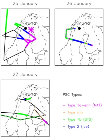
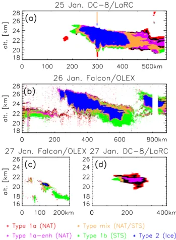
Figure 3 shows an overview of the lidar measurements on 25–27 January. The lidar data was classified with the clas-sification of Biele et al. (2001) and shows PSCs over Scan-dinavia on all 3 successive days. Figure 4 shows the flight path of the selected lidar data segments, and Fig. 5 shows the results of the classification of these data segments according to Biele et al. (2001).
4.1 25 January 2000
The DC-8 crossed the Scandinavian mountain ridge three times, and on each crossing PSCs were observed, consist-ing of ice, STS, and likely NAT (see Fig. 3). The LaRC lidar
Fig. 3. Overview of lidar data 25–27 January 2000, classification
according to Biele et al. (2001). Black lines show flight path without PSC observations, colored lines show flight path with PSC observa-tions (color codes as indicated, dashed line segments indicate small PSC patches and/or two PSC types at the same position). 25 Jan-uary: LaRC (NASA) lidar data, “*” indicates balloon-borne mea-surements of Voigt et al. (2000). 26 January: OLEX (DLR) lidar data. 27 January: LaRC (NASA) and OLEX (DLR) lidar data.
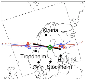
Trondheim
Kiruna
Narvik
Helsinki
Fig. 4. Flight path segments of lidar data presented in this study,
arrows indicate flight direction. Solid line: DC-8, 25 January 2000, 15:03–15:38 UTC; dotted line: Falcon, 26 January 2000, 13:58– 14:51 UTC (flight leg 3); dashed line: Falcon, 27 January 2000, 13:36–13:59 UTC and DC-8, 27 January 2000, 12:53–13:30 UTC.
and the ice particles evaporate. Depending on temperature, also the liquid ternary solution droplets evaporate HNO3and develop back to binary H2SO4/H2O droplets. Eventually, the NAT particles evaporate when the temperature rises above the existence temperatureTNAT, which is about 8 K above
Tice(Hanson and Mauersberger , 1988). Zondlo et al. (2000) provide a comprehensive overview over these processes.
Based on the LaRC lidar data, Hu et al. (2002) estimated ice particle number densities in this PSCnice =2−5 cm−3 with a mode radiusr = 1.2−2µm. NAT particle num-ber densities were estimated asnNAT=0.1−0.5 cm−3with a mode radiusr = 0.4−1µm, in general agreement with our analysis (not shown). Balloon-borne in-situ measure-ments on this day at 20:30–22:30 UTC (see Fig. 3) show the presence of STS and NAT particles downwind of the Scandinavian mountain ridge at altitudes 22-23 km, with a NAT particle number density ofn ≈0.1 cm−3and a radius
r=0.5 −1µm (Voigt et al., 2000). 4.2 26 January 2000
Lidar observations on board of the Falcon aircraft show the presence of large ice PSCs over Scandinavia and patches of STS and type 1a-enh PSCs over the Atlantic ocean. Down-stream of the large ice cloud over Scandinavia (see Fig. 5b, at 200 - 600 km, and Fig. 3) the Falcon observed a sec-ond ice PSC over Finland (see Fig. 5b, at 750-850 km, and Fig. 3). This rather unique observation of 2 large suc-cessive PSCs was chosen as a test case for the combined mesoscale/microphysical modeling approach (Sect. 5). The first ice PSC was also observed by ground-based FTIR, and based on the FTIR data, Hoepfner et al. (2001) estimated the average ice particle number densitiesnice =2-5 cm−3, with a corresponding particle radius r = 2−1µm, in general
Fig. 5.Classification of lidar data according to Biele et al. (2001).
Color codes as indicated, black areas cannot be assigned to a class. Wind direction from left to right, except panel (d) with perpendic-ular wind. (a)Classification of LaRC lidar observation on board the NASA DC-8 aircraft, 25 January 2000, 15:03–15:38 UTC.(b) Classification of OLEX lidar data on board the DLR Falcon aircraft, 26 January 2000, 13:58–14:51 UTC.(c)Classification of OLEX li-dar data, 27 January 2000, 13:36–13:59 UTC.(d)Classification of LaRC lidar data, 27 January 2000, 12:53–13:30 UTC. Data seg-ments correspond to flight paths in Fig. 2.
agreement with the analysis presented in Sect. 5. Directly downstream of the first ice PSC, following a small region of type “mix”, only a tiny margin of the PSC is identified as type 1a/1a-enh (see Fig. 5b, at 300-650 km and 22-26 km alt.). A few isolated NAT “streaks” leave the lower part of the first ice cloud (see Fig. 5b at∼ 700 km). The PSC up-stream of the first ice cloud (see Fig. 5b, at 0-200 km, altitude ≈22 km) is classified as 1a-enh/mix/STS and is part of sev-eral stratified PSC patches observed at≈22 km altitude over the Atlantic (see Fig. 3).
ice cloud), if present at all, must be small (r <0.5µm) and in very low number densitiesnNAT ≈0.01 cm−3, such that the liquid droplets dominate the lidar backscatter.
4.3 27 January 2000
On 27 January PSCs were sparse compared to the two pre-ceding days. At 13:45 UTC the Falcon observed a small (≈ 30 km in wind direction) ice PSC near Kiruna, about 50 km downstream of Kebnekaise, the highest peak in northern Scandinavia (18◦33’E/ 67◦53’N, elevation 2111 m). Down-stream of and just below the ice PSC there is STS (see Figs. 3 and 5c). The small geographical dimensions of the cloud in-dicates that in general temperatures were above the ice nucle-ation temperature, but single mountains such as Kebnekaise may generate gravity waves of small horizontal dimensions and thus localized cooling.
The DC-8 headed south from Kiruna and observed a PSC near Helsinki/St.Petersburg (13:00–13:15 UTC, Figs. 3 and 5d). On the subsequent crossing of the mountain ridge, only STS was observed. The cloud near Helsinki classifies as type 1a-enh, type 1a and a small section as type 1b (STS). A hy-pothesis for the genesis of this NAT cloud will be presented in Sect. 6.
In addition to the lidar data, in-situ measurements on board the NASA ER-2 stratospheric research aircraft are available for this day. The ER-2 left Kiruna at ∼09:00 UTC and headed south over Finland towards Russia, from where it returned to Kiruna. During the entire flight, the NOy in-strument found particulate matter at two positions only: on the outbound flight at∼10:00 UTC, 27.83◦E/61.44◦N, and
on the incoming flight at ∼13:15 UTC, 29.45◦E/59.9◦N.
The two locations are in agreement with the lidar observa-tion of the type 1a-enh PSC discussed above. Based on the NOydata, Northway et al. (2002) estimated a particle radius
r ≈ 3µm (outgoing flight leg) andr ≈ 4µm (incoming flight leg) in low number densitiesnNAT ≈ 3×10⁻⁴cm−3. T-Matrix calculations for NAT particles of these sizes and number densities yield a backscatter ratio BSR(1064).1.25, which is far from the observed values BSR(1064)≈3-15. The observed color ratio CR(532/1064) ≈1.1-3 of the li-dar observation indicates that the cloud mainly consists of smaller particles (from T-Matrix calculations we estimate
r ≈0.8µm,nNAT≈0.3 cm−3, corresponding to∼3 ppmv HNO3in the solid phase). This discrepancy between in-situ NOy and lidar data may be resolved by the fact that the al-titude of the ER-2 measurement (∼20 km) is at the extreme bottom of the PSC observed by the lidar (see Fig. 5d). It can be speculated whether these larger particles at the cloud bottom result from sedimentation processes as proposed by Fueglistaler et al. (2002a); Dhaniyala et al. (2002). In ad-dition, the NAT number densities at the edges of the cloud may be smaller due to less favorable nucleation conditions at cloud formation time. Both processes can lead to the ob-served low number density. In sum we may conclude that
Trondheim
Kiruna
Helsinki
Oslo Stockholm
Fig. 6. Falcon flight path and air parcel trajectories on 26 January
2000, and domain boundaries of the mesoscale model HRM (black dash-dotted lines). Black solid line: Falcon flight path (leg 3, flight direction from west to east, 13:58–14:51 UTC). Colored lines: isen-tropic forward and backward trajectories on 500 K (red) and 600 K (blue), started at 20.37◦E/63.75◦N, 15:00 UTC (green diamond). Dotted lines: ECMWF trajectories. Solid lines: HRM trajectories. Wind direction from West to East, triangles indicate trajectory po-sitions at 10:00 UTC, and crosses popo-sitions at 18:00 UTC.
this cloud consists of NAT particles withr . 4µm, most likely withr≈0.8µm andnNAT≈0.3 cm−3.
5 Detailed PSC modeling, 26 January 2000
A comprehensive microphysical box model (Luo et al., 2002) was used with trajectories from NWP models. For-ward and backFor-ward trajectories were calculated starting at 20.37◦E/63.75◦N, 15:00 UTC between 400 K and 650 K potential temperature in increments of 2 K (corresponding to a vertical resolution∼100 m, yielding a total of 126 tra-jectories), from both ECMWF analysis data and the HRM simulation.
450 K 500 K 550 K 600 K
Fig. 7. (a)OLEX lidar data (BSR 1064 nm), 26 January 2000,
and selected trajectories calculated from ECMWF analysis data (black dashed lines) and the HRM simulation (black solid lines). White solid line: manually modified (based on the lidar image) HRM trajectory (550 K). Trajectories started at 20.37◦E/63.75◦N, 15:00 UTC on the labelled isentropes.(b)Lidar signal (BSR 1064 nm) inferred from microphysical model calculations along the 126 trajectories between 400 K and 650 K calculated with the HRM mesoscale simulation. (c) Lidar signal (BSR 1064 nm) inferred from microphysical model calculations along the 126 trajectories between 400 K and 650 K calculated with ECMWF analysis data.
The simulated backscatter ratio BSR(1064) based on the results of the microphysical calculations along the trajecto-ries is shown in Fig. 7 together with the measured backscatter ratio BSR(1064). This allows a direct comparison of simu-lations and measurements, while the underlying microphyis-cal results, such as particle types and number densities, are shown later (see Fig. 9). Model results along trajectories are plotted in the geometry of the flight path (positions are re-sampled to equal distance from the reference position where flight path and all trajectories intersect).
A comparison of the HRM-based PSC simulation (Fig. 7b) with the measured lidar signal (Fig. 7a) shows that the simu-lation is in good agreement with the measurement. In par-ticular, the shape of first ice cloud over Scandinavia fits the observation very well, and hence corroborates the HRM mesoscale simulation in combination with the modeling of
the ice nucleation. Also the second ice cloud is in general agreement with measurements, although its shape shows a tilt westward with height which is too strong compared to the measurement. Measured and simulated lidar backscatter ratios agree well and deviations are on average less than 25%. We conclude that the mesoscale/microphysical model simu-lation correctly reproduces the cloud microphysics, in partic-ular the particle types, number densities and sizes. It is em-phasized again at this point that the simulation uses the me-teorological parameters temperature and pressure from the HRM simulation without any modification, and that the mi-crophysical box model calculates the nucleation of ice and NAT particles from nucleation rates rather than from pre-scribed values as in previous studies.
Upon closer inspection of measurement and simulation we note again the wrong tilt of the second ice cloud. A part of this tilt is an effect of the deviation between flight path and trajectories, however it is also apparent in the temperature field of the HRM simulation. This tilt is also observed in the main ice cloud, where it causes trajectories to descend too soon compared to the measurement (i.e. ice particles evap-orate too soon in the simulation, compare the ice regions with BSR(1064) > 100 at 24-25 km altitude in the mea-surement and simulation, Figs. 7a,b). Further we note that the HRM-based simulation cannot reproduce the small scale waves (with wavelength.20 km and amplitude.5 K) su-perimposed on the dominant wave number observed in the lidar data. It is clear that the mesoscale model with a spatial resolution of ∼ 15 km cannot resolve these waves. Calcu-lations with a manually modified trajectory with these small scale waves superimposed on the HRM trajectory show that these waves can affect the microphysical properties quanti-tatively, but do not change the qualitative properties of the cloud (calculations shown in the Appendix).
The simulation cannot reproduce the small PSC at 22 km altitude upstream of the first ice cloud, in Sect. 4.2 identified as STS and NAT, due to two reasons. Firstly, the microphys-ical model requires ice particles to initiate NAT nucleation, but the HRM simulation temperatures do not reach the ice nucleation temperature upstream of Scandinavia. Secondly, the HRM backtrajectories are slightly further south than the flight path for this section over the Atlantic (see Fig. 6). As will be shown later, a trough of air cold enough to form STS is present in the simulation at the location where the upstream PSC was observed, but its southern edge is just missed by the HRM trajectories.
Fig. 8. (a)Minimum temperatures along trajectories from HRM simulation (solid line) and ECMWF analysis (dotted line), and the corresponding ice existence temperatures (dashed line: HRM sim-ulation; dash-dotted line: ECMWF analysis);(b)Maximum satu-ration ratio of gas phase with respect to NAT in the presence of ice, again along trajectories from HRM simulation (solid line) and ECMWF analysis data (dotted line), calculated with the microphys-ical box model.
HRM trajectories. Again, trajectories do not reach the ice nucleation temperature further upstream, and consequently the microphysical model fails to produce the observed NAT particles. A hypothesis on the origin of these NAT clouds is beyond the scope of this paper, but we note that these clouds might be a challenge to test hypotheses on NAT nucleation.
Figure 8 shows an overview of the minimum tempera-tures and the calculated maximum NAT saturation ratios in the presence of ice (SNAT) along the trajectories used for this simulation. As expected from the lower spatial reso-lution, ECMWF analysis underestimates orographically in-duced temperature deviations from synoptic scale tempera-tures. In addition, the underestimation of the wave ampli-tude yields NAT supersaturations considerably lower than the HRM-based trajectories. The latter yield very high NAT su-persaturations ofSNAT & 200, in agreement with the high supersaturations found in manually constructed trajectories by Luo et al. (2002).
Figure 9a shows the maximum cooling rates found in the HRM trajectories and ECMWF trajectories. The latter cannot reproduce the strong cooling rates found in moun-tain gravity waves and remain below 10 K/h. In contrast, the HRM trajectories show maximum cooling rates of 30– 50 K/h, in accordance with manually constructed trajecto-ries (Luo et al., 2002). The maximum cooling rates largely control the STS aerosol. With high cooling rates&20 K/h the H2O/HNO3uptake of the STS droplets cannot keep pace with the decrease in vapor pressure, and the STS aerosol is out of equilibrium with the surrounding gas phase, resulting in extremely high NAT supersaturations with respect to ice as shown in Fig. 8b.
Figure 9b shows the cooling rates of the HRM-based tra-jetories at the onset of ice nucleation, which controls the resulting ice particle number density. The largest droplets are to freeze first (due to their volume) and begin to
de-Fig. 9. (a)Maximum cooling rates along trajectories from HRM
simulation (black solid line) and ECMWF analysis data (black dot-ted line). (b)Cooling rate of the HRM trajectories at the onset of ice nucleation (black crosses) and the range of cooling rates within 15 min before (dark gray area) and 3 min after nucleation (light gray area).
Fig. 10. Solid particle number densities in the PSC simulation of
26 January 2000 (based on HRM simulation). Dark gray shading: NAT number density. Light grey shading: ice number density.
plete the gas phase. As a result, the ice saturation ratio (Sice = ppart/pvapor) decreases. When the saturation ratio falls below the supersaturation required for ice nucleation, further ice nucleation is inhibited. At high cooling rates
&15 K/h the decrease in partial pressure is compensated or even overcompensated by a decrease in vapor pressure, such that all droplets freeze (we will refer to this as 100% ice acti-vation). The majority of cooling rates at onset of nucleation in the HRM trajectories is in the range 10–25 K/h. Conse-quently, most trajectories show∼ 100% ice activation, de-spite the fact that nucleation begins at cooling rates signifi-cantly lower than the maximum values along the trajectories. In most cases, the cooling rate further decreases during the next 3 min after onset of nucleation, but still remains too high in most cases to restrict resulting ice particle number density. The 3 min timeframe is motivated by the priod of continuous nucleation, which ranges from a few tens of seconds (rapid cooling) to a few minutes (slow cooling).
nucleation occurs. This is different for NAT nucleation on ice. The generally lower cooling rates at altitudes of 500– 550 K (see Fig. 9b) allow the liquid aerosol to grow to larger sizes, and supersaturations with respect to NAT remain lower than at higher altitudes. Consequently, the NAT nucleation rate calculated according to Luo et al. (2002) is lower, result-ing innNAT≈0.1−0.5 cm−3. At higher altitudes the simu-lations yield NAT number densities ofnNAT≈2−8 cm−3.
In order to quantify the accuracy of the modeled NAT and ice number densities, a detailed analysis of the lidar observa-tions has been performed and is shown in the Appendix. The basic conclusion is that the mesoscale/microphysical model yields results in general agreement with measurements, and that the temperatures and cooling rates of mesoscale models such as HRM suffice to model mountain wave PSCs.
6 Modeling of PSC evolution, 25–27 January 2000
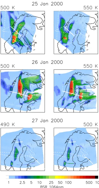
In the previous section it was shown that the combined mesoscale/microphysical modeling approach yields results in good agreement with observations. Now we will use this approach to model the 3-dimensional evolution of the PSCs on 25–27 January 2000. Similar to the previous simulation we calculated trajectories from the HRM simulation and used these trajectories as input for the microphysical boxmodel. For this simulation we calculated for each day 200 trajecto-ries on two potential temperature levels, started along a line from 12◦E/59◦N to 28◦E/72◦N. Based on the altitude level of PSC observations in the lidar data, simulations for 500 and 550 K potential temperature are shown for 25 and 26 Jan-uary in Figs. 11 and 12. On 27 JanJan-uary the simulations for 490 and 500 K are shown. Based on the times of the lidar observations, trajectories were started 15:00 UTC for 25 and 26 January and 11:00 UTC for 27 January.
6.1 25 January 2000
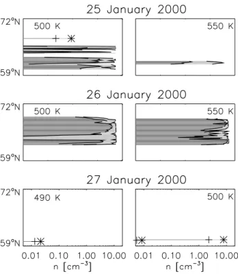
The simulations show STS, NAT and ice clouds both on the 500 K and 550 K level. From a comparison with measure-ments (see Fig. 3), it is apparent that the simulation overes-timates temperatures over northern Scandinavia by 1–3 K. The simulations show mainly STS in this region, whereas the measurements show a large ice PSC near Kiruna. The ice PSCs over central Scandianvia are correctly modeled (indi-cated in Fig. 11 by BSR(1064)> 50, see also Fig. 12). An inspection of NAT number densities in the trajectories that fit best the track of the balloon-borne experiment (near Kiruna) presented by Voigt et al. (2000) shows NAT number densities
nNAT≈0.1 cm−3. This value is in good agreement with the measurednNAT≈0.1 cm−3(Voigt et al., 2000). Over central Scandinavia, the simulation yieldsnNAT =0.2-3 cm−3(see Fig. 12), which is also in good agreement with the results of the analysis of lidar data by Hu et al. (2002), who estimated for this regionnNAT=0.1−0.5 cm−3.
Fig. 11. BSR(1064) calculated from results of combined
mesoscale/microphysical modeling on two isentropic levels for 25– 27 January 2000. Trajectories were started along a straight line from 12◦/60◦to 28◦/72◦at 15:00 UTC of each day (except for 27 January, where trajectories were started at 11:00 UTC). The different trajec-tory starting time and isentropes of 27 January account for the PSC observation times and altitude range of this day. White solid lines: flight legs discussed in this study (25 January: DC-8; 26 January: Falcon; 27 January: Falcon and DC-8). White dotted lines: en-tire flight path (25 January: DC-8; 26 January: Falcon; 27 January: DC-8).
6.2 26 January
Fig. 12. Solid particle number densities in the simulations. Dark gray: NAT number density. Light grey: ice number density. All panels use the same axes, the values of the individual trajectories are plotted versus the latitude of the starting position. On 27 Jan-uary only 3 trajectories show ice. To better visualize the data, “+” indicates NAT number density and “*” indicates ice number density where necessary.
on the 500 K and 550 K isentropes. These simulations fur-thermore show that NAT clouds downstream of the northern part of the first ice PSC prevail until the trajectories leave the domain of the simulation (the region with BSR(1064)≈15, identification of NAT in the simulation after inspection of the data of the microphysical simulation, Fig. 12). The pres-ence of a region where the NAT PSC evaporates∼200 km downstream of the ice cloud highlights again the fact that, de-pending on the temperature history, NAT can also be absent downstream of an ice PSC. It was earlier mentioned that the simulation of the vertical cross-section of 26 January based on HRM data does not show the observed STS cloud up-stream of the ice PSC. The simulations shown here support the explanation suggested earlier that the slight displacement of the flight path and the trajectories is responsible for the disagreement. The horizontal simulation reveals a pool of cold air located over the Atlantic, giving rise to STS clouds (BSR(1064)≈3, identification of STS after inspection of the data of the microphysical simulation). The simulated STS cloud is in agreement with observed STS clouds (see Fig. 3), and ceases to exist at approximately the latitude where the Falcon aircraft turned eastward.
6.3 27 January
The simulation of this day misses the small ice PSC∼50 km downstream of Kebnekaise (18◦33’E/67◦53’N, elevation 2111 m), but correctly predicts the observed STS cloud at the same location. Apparently, the HRM model slightly overes-timates temperatures in this region. Considering the limited horizontal resolution (∼15 km) of the HRM model and the smoothed orography, it seems plausible that the model un-derestimates gravity waves caused by high, but horizontally small orographic features such as Kebnekaise.
The presence of an STS cloud over central Scandinavia in the simulation (with BSR(1064). 10) is confirmed by the LaRC measurements on board the DC-8 (see Fig. 3). The simulation does not show the observed NAT PSC near Helsinki/St. Petersburg (see Figs. 3 and 5d), but holds a plau-sible explanation for the cloud. The simulation shows the presence of a small ice cloud over southern Scandinavia (near Oslo), which gives rise to a NAT cloud downstream (the small line in the horizontal simulation with BSR(1064) = 2−10, identification of NAT after inspection of the data of the microphysical simulation, Fig. 12). In the simulation, temperatures further downstream are slightly too high such that the NAT particles evaporate shortly before the air trajec-tory intersects with the flight path. We have refrained from lowering the temperatures by∼1 K which would be required to produce a ‘match’ with the observed type 1a-enh PSC, to remain in accordance with all other simulations where all meteorological parameters of the NWP models remained un-altered. An inspection of the data of the microphysical simu-lation (see Fig. 12) shows a number density of the ice cloud near Oslonice =0.01−8 cm−3(i.e. also very slow cooling rates at the onset of nucleation). The simulated NAT cloud downstream showsnNAT=0.01−2 cm−3(i.e. a large range of number densities), which is in agreement with our earlier calculations based on the measured lidar data, which con-cludednNAT≈0.3 cm−3andr≈0.8µm.
7 Conclusions
The model simulations use trajectory calculations based on mesoscale simulations with the High Resolution Model (HRM) as input for our microphysical box model. All mi-crophysical calculations use the meteorological information of the trajectories without modifications (i.e. without “tun-ing” of the temperature). We calculate a lidar signal from the microphysical simulation with T-Matrix calculations for aspherical particles and Mie calculations for liquid particles. The comparison of simulations and measurements shows:
a The mesoscale HRM simulations of orographically in-duced gravity waves over Scandinavia are in good agreement with lidar observations. As a general ten-dency, the wave amplitude appears to be slightly un-derestimated rather than overestimated, such that the simulations do not always yield ice when observations indicate the presence of ice. However, in general the mesoscale simulation captures minimum temperatures and cooling rates well. Sensitivity studies (not shown) show that the results of the mesoscale modeling are ro-bust, i.e. that for different model setups the results do not critically differ. We conclude from this study that the mesoscale modeling is sufficiently reliable to model the microphysics of mountain wave ice PSCs over Scan-dinavia, even though it still misses very small ice clouds which may be caused by orographic features that are ei-ther not present in the model orography or cause gravity waves which cannot be resolved even with a horizontal resolution of∼15 km.
Simulations with ECMWF analysis data show that the model, as a consequence of its synoptic scope and coarse resolution, severely underestimates lowest tem-peratures and cooling rates. Consequently, ECMWF data (and data of other NWP models with similar spatial resolution) are only suited for the study of liquid PSCs on a synoptic scale.
b The simulations show that in mountain wave PSC events the ice PSC observations are in agreement with simulations assuming homogeneous ice nucleation and using the parametrization of Koop et al. (2000). The accuracy of the mesoscale trajectory calculations is not sufficient to resolve details of the ice PSCs, but on a statistical basis the simulations yielded both ice number densities and particle sizes within the range of observa-tions. We estimate the accuracy of the modeled particle number densities within a factor 2 for ice particles. A more precise estimation of the accuracy is not (yet) pos-sible due to the uncertainties in the interpretation of the (lidar) data.
c This modeling study assumes NAT nucleation on ice ac-cording to the process described by Luo et al. (2002). All observations of NAT in the region of interest could be explained with this process except patches of NAT
clouds over the Atlantic, which we have not further an-alyzed in this study. This study supports the assumption that NAT forms in (mountain wave) ice PSCs, though it does not exclude other nucleation mechanisms. The accuracy of the modeled NAT number density is esti-mated to be within a factor 10, the uncertainty again largely caused by uncertainties in the interpretation of the measurements. The importance of combined in-situ and lidar measurements to finally overcome limitations in the lidar data retrieval cannot be overemphasized.
d If NAT nucleation on ice is of importance to the deni-trification of the polar stratosphere (e.g. via sedimen-tation of NAT particles out of high number density NAT clouds as proposed by Fueglistaler et al., 2002a,b; Dhaniyala et al., 2002), then Chemical Transport Mod-els (CTM) using synoptic scale temperature and wind fields miss a key element in the process of ozone de-struction. Ice PSCs cannot be simulated realiably with synoptic scale temperature fields, and consequently the formation of NAT particles, their sedimentation and the resulting denitrification is not accurate.
In summary, this study shows that the combined mesoscale/microphysical modeling approach yields results in good agreement with observations and enables the inves-tiagation of the 3-dimensional structure of mountain wave PSCs. The results of this approach are the first of their kind and show a level of detail in the modeling and comparison with measurements not performed before. It is shown that the current understanding of PSC microphysics and mesoscale dynamics modeling suffices to explain the key characteristics of mountain wave PSC events. However, the study also im-plies that currently available data do not suffice to draw new conclusions about the microphysics of PSCs (despite the ex-cellence of the SOLVE/THESEO-2000 campaign data). It is conceivable that future Arctic campaigns use not only meteo-rological forecasts, but also microphysical calculations based on mesoscale forecasts to guide mission planning. This ap-proach could contribute to observations that allow to reject or prove suggested microphysical processes in PSCs, and hence to a significant improvement of our understanding of PSC formation.
Appendix: Detailed lidar data retrieval 26 January 2000
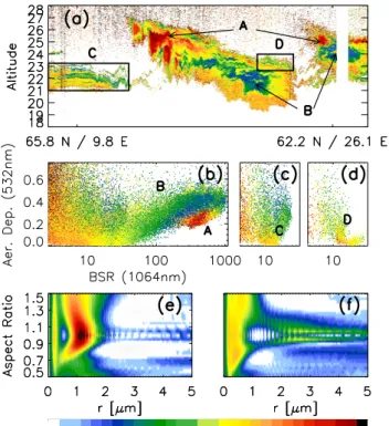
Figure 13 shows the measured color ratio CR(532/1064), scatterplots of the data in the δaer(532)/BSR(1064) plane (Figs. 13b, c, d) together with color ratios calculated with the T-Matrix method for ice and NAT particles (Figs. 13e, f; the particle shape is a spheroid with aspect ratio 0.5 to 1.5).
Fig. 13. (a)Color ratio CR(532/1064) of OLEX measurement on 26 January 2000 (leg 3). The regions A–D are discussed in text.(b) Scatterplot of lidar data of 26 January 2000 (leg 3). Note that the high color ratio value region at BSR(1064)=200−800 is partially covered by points with lower color ratios. (c)Scatterplot of lidar data of region C.(d) Scatterplot of lidar data of region D.(e) T-Matrix calculation of CR(532/1064) for spheroids, ice.(f)T-Matrix calculation of CR(532/1064) for spheroids, NAT.
color ratio and a tendency towards lower aerosol depolariza-tion (see Fig. 13b) compared to region “B” (note that the plot-ting in a scatterplot leads to an overplot of a small fraction of data with high color ratio and high aerosol depolarization). Regions “C” and “D” cover areas of interest with respect to the occurrence of NAT particles. Data of these regions cannot be unequivocally identified in the scatterplot due to noise in the depolarization data at BSR(1064).5 (probably caused by an iced window, H. Flenje, pers. comm.).
Ice particles
The observed difference in color ratio in the ice cloud be-tween regions above∼ 23 km (“A”) and below (“B”) indi-cates that the sizes of the ice particles in the two regions differ. Region “A” shows a high backscatter and a color ratio CR(532/1064) = 5−9. Based on the T-Matrix cal-culations shown in Fig. 13e, we estimate ice particle sizes
r = 1 − 1.5µm (with aspect ratio∼ 0.9) in this region. In thermodynamic equilibrium atT ≈Tice−3 K a particle size ofr ≤ 1.5µm requiresnice ≥ 10 cm−3. This implies
that basically the entire background aerosol froze, which in turn requires cooling rates>10 K/h at the onset of ice nucle-ation (based on sensitivity studies for different cooling rates, calculated with the microphysical box model). The calcu-lated ice number densities in the simulation in this region of
nice=10−12 cm−3(see Fig. 10) agree well with these con-siderations based on the lidar data.
Region “B” shows a similar BSR(1064) as region “A”, but has a significantly lower color ratio CR(532/1064)<1.5. An inspection of the T-Matrix calculations (see Fig. 13e) shows that the observations can be explained by ice particles of size
r &1.8µm and aspect ratio 0.9, with a corresponding par-ticle number densitynice . 5cm−3. Calculations show that altitude-dependent variations in available water vapor affect ice particle sizes, but cannot be the only reason for the differ-ent color ratios of regions “A” and “B”. Rather, we consider a different particle shape of ice particles in the two regions a likely cause. Figure 13e shows that particles with aspect ra-tio∼0.65 show moderate color ratios CR(532/1064).2 for practically all particle sizes. This is in accordance with the fact that a distinct peak in color ratio, as expected for growing ice particles with aspect ratio&0.8, is not observed in region “B”. In principle, also very slow cooling rates (.2.5 K/h) could lead to the observed low color ratios, even for parti-cles with aspect ratio 0.85. Cooling rates.2.5 K/h lead to
nice .1 cm−3ice particles, which follow a wide size distri-bution, such that the distinct peak in color ratio atr≈1µm diminishes. An estimation of cooling rates based on the li-dar data of the STS cloud upstream of the ice cloud yields an average cooling rate∼10 K/h (in agreement with the HRM simulation, Fig. 8b), which is considerably higher than the required 2.5 K/h. Even under the assumption of lower cool-ing rates at the begin of nucleation, an aspect ratio∼0.85 for ice particles appears unlikely. Minor variations in the cooling rate of±1 K/h (which can be safely expected for the strato-sphere) inevitably lead to variations in particle number den-sity that cause significantly higher than observed color ratios. Thus, we consider differing aspect ratios in region “A” and “B” the most likely hypothesis for the systematic difference in color ratio.
On the reason for a systematic difference in particle shapes of region “A” and “B” we can only speculate. As out-lined above, cooling rates are lower upstream of region “B” (though still high enough to freeze most of the background aerosol). Consequently, the ice particles of region “B” nucle-ated in larger droplets and grew in an environment closer to the thermodynamic equilibrium, which could favour crystal growth along the preferred axes, and hence a more prolate shape.
the observation (see Fig. 7b). On the other hand, the mean cooling rates upstream of region “B” appear realistic from a comparison of the horizontal dimensions of the STS up-stream of region “B”. Yet, the cooling rates at the location of ice nucleation is still too high (see Fig. 9b) to severly reduce the number of freezing particles (see Fig. 10). The extreme sensitivity of ice nucleation rates on cooling rates would re-quire trajectories with an accuracy in cooling rates within ±0.5 K/h, which is far beyond from what current NWP mod-els can deliver.
NAT particles
The lidar classification discussed in Sect. 4.2 shows a sub-stantial fraction of pixels directly downwind of the ice cloud (region “D”) classified as “NAT” or “mixed”, but the signal is noisy. Here we compare the signal in the two regions “C” and “D” (Figs. 13c, d). Region “C” is clearly classified as STS, “mix” and a layer of NAT particles. The layer dominated by NAT shows a distinct color ratio CR(532/1064)=1−2, whereas the other parts of region “C” show CR(532/1064)&
3.25. A comparison with T-Matrix calculations (Fig. 13f) shows that the observed signal (significant depolarization and color ratio CR(532/1064)=1−2) is in agreement with NAT particles withr & 0.5µm. The observed backscatter ratio BSR(1064)=5−30 indicatesnNAT =0.5−3 cm−3NAT particles (with r = 0.5µm), with a corresponding HNO3 mixing ratio 1–5 ppbv in the solid phase.
Region “D” shows similar aerosol depolarization as region “C”, but a lower backscatter ratio (BSR(1064)=5−15) and color ratios CR(532/1064)=1.5−3.25. This indicates that region ‘D’ contains NAT particles with a sizer . 0.5µm and particle number densities ofn=0.5−10 cm−3, corre-sponding to<3 ppbv HNO3in the solid phase. This anal-ysis shows thatn=0.5−10 cm−3NAT particles may well be present downwind of the ice PSC, but the period of time where temperatures are too high for STS but still belowTNAT is too small to cause a clear 1a-enh classification.
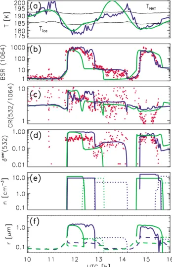
Simulation results of a manually optimized trajectory Figure 14 shows a detailed comparison of microphysical and optical parameters between model calculations along the HRM 550 K trajectory and a manually modified trajectory (based on the 550 K HRM trajectory and lidar data interpre-tation; the white line in Fig. 7a shows the location of the tra-jectory in the geometry of the lidar data). The figure shows that much of the inconsistency between measured lidar sig-nal and HRM-based simulations can be explained by a few shortcomings in the HRM trajectory. In particular, the spa-tial wavelength of the main gravity wave over Scandinavia is underestimated in the HRM simulation, and temperatures of the manual trajectory remain longer belowTice(see Fig. 14a), and hence ice particles prevail.
Fig. 14. Comparison of microphysical simulations along HRM
550 K trajectory, manually modified HRM trajectory (550 K), and lidar measurement along the modified trajectory. (a) Tempera-ture of HRM trajectory (green) and modified trajectory (blue);(b) BSR(1064) along trajectories. Red dots: OLEX measurement along manually adjusted trajectory; blue line: calculated lidar signal along modified trajectory; green line: calculated lidar signal along HRM trajectory. The lidar backscatter calculations use spheroids with as-pect ratio 0.85 for ice and 0.75 for NAT.(c)Lidar color ratio (532 nm/1064 nm, colors as in (b). Calculations for second ice cloud use aspect ratio 0.7 for ice particles. (d)Aerosol depolarization (532 nm), colors as in (b). Calculations for second ice cloud use as-pect ratio 0.7 for ice particles. (e)Number densities of ice (solid) and NAT (dotted), colors as in (b). (f)Particle mode radius of ice (solid), NAT (dotted) and liquid (dashed), colors as in (b).
in good agreement with the observed variation of BSR(1064) in the ice cloud. While the simulated backscatter ratio at 1064 nm is in good agreement with observations (indepen-dently of aspect ratio), it is more difficult to correctly model CR(532/1064) and aerosol depolarization. Figures 14b and c show the observed and simulated color ratios and aerosol depolarizations. For the second ice cloud, which has a lidar signal similar to the earlier discussed region “B”, we used an ice particle aspect ratio 0.7, in accordance with our ear-lier considerations (all other calculations used an aspect ratio 0.85 for ice particles). The calculation with aspect ratio 0.85 for ice particles is in good agreement with measured color ratios in the first ice cloud, but overestimates aerosol depo-larization. In contrast, the calculation with aspect ratio 0.7 for the second ice cloud is in good agreement with observed aerosol depolarization, but overestimates color ratios.
As a result of the rapid cooling, the model yields down-wind of the first ice PSC (at ∼13–14:00 UTC) nNAT ≈ 10 cm−3 NAT particles (i.e. on most ice particles a NAT particle nucleated). Backscatter, color ratio and depolariza-tion of the secdepolariza-tions where NAT particles prevail are in gen-eral agreement with the observations. Deviations may be ex-plained by the fact that it is difficult to follow the air flow in the lidar image, and consequently the manual trajectory is not perfectly quasi-Lagrangian (note the increased scatter in the lidar data around 13:30–14:00 UTC). Downwind of the second PSC the simulation yieldsnNAT=5−10 cm−3NAT particles (again almost 100 % activation).
In summary, the manually modified trajectory improves the agreement between simulation and measurement, but does not fundamentally change the results obtained with the HRM trajectories. The original HRM trajectory may not be able to resolve details, but yields particle number densities and sizes very similar (within a factor 2) to the manually optimized trajectory. From this detailed analysis we con-clude that the combined mesoscale/microphysical modeling approach yields results in general agreement with measure-ments, and that temperatures and cooling rates of mesoscale models such as HRM suffice to model mountain wave PSCs.
Acknowledgements. SF and SB have been supported through
the EC-project THESEO-2000/EuroSOLVE (under contract BBW 99.0218-2, EVK2-CT-1999-00047) and through an ETHZ-internal research project. BL has been supported through the EC-project MapScore. We thank D. L¨uthi for his help with the setup of the HRM model. We thank A. D¨ornbrack, C. Schiller, T. Deshler, and C. Voigt for fruitful discussions.
References
Biele, J., Tsias, A., Luo, B. P., Carslaw, K. S., Neuber, R., Bey-erle, G., and Peter, Th.: Nonequilibrium coexistence of solid and liquid particles in Arctic stratospheric clouds, J. Geophys. Res., 106, 22991–23007, 2001.
Browell, E. V., Butler, C. F., Ismail, S., Robinette, P. A., Carter, A. F., Higdon, N. S., Toon, O. B., Schoeberl, M. R., and Tuck,
A. F.: Airborne Lidar Observations In The Wintertime Arctic Stratosphere: Polar Stratospheric Clouds, Geophys. Res. Lett., 17, 385–388, 1990.
Carslaw, K. S., Luo, B. P., Clegg, S. L., Peter, Th., Brimblecombe, P., and Crutzen, P. J.: Stratospheric aerosol growth and HNO3
gas phase depletion from coupled HNO3 and water uptake by
liquid particles, Geophys. Res. Lett., 21, 2479–2482, 1994. Carslaw, K. S., Wirth, M., Tsias, A., Luo, B. P., D¨ornbrack, A.,
Leutbecher, M., Volkert, H., Renger, W., Bacmeister, J. T., and Peter, Th.: Particle microphysics and chemistry in remotely ob-served mountain polar stratospheric clouds, J. Geophys. Res., 103, 5785–5796, 1998a.
Carslaw, K. S., Wirth, M., Tsias, A., Luo, B. P., D¨ornbrack, A., Leutbecher, M., Volkert, H., Renger, W., Bacmeister, J. T., Reimer, E., and Peter, Th.: Increased stratospheric ozone deple-tion due to mountain-induced atmospheric waves, Nature, 391, 675–678, 1998b.
Dhaniyala, S., McKinney, K. A., and Wennberg, P. O.: Lee-wave clouds and denitrification of the polar stratosphere, Geophys. Res. Lett., 29, 9, 1322, doi:10.1029/2001GL013900, 2002. D¨ornbrack, A., Leutbecher, M., Kivi, R., and Kyr¨o, E.:
Moun-tain wave-induced record low stratospheric temperatures above northern Scandinavia, Tellus, 51A, 951–963, 1999.
D¨ornbrack, A., Leutbecher, M., Reichardt, J., Behrendt, A., M¨uller, K.-P., and Baumgarten, G.: Relevance of mountain wave cooling for the formation of polar stratospheric clouds over Scandinavia: Mesoscale dynamics and observations for January 1997, J. Geo-phys. Res., 106, 1569–1581, 2001.
D¨ornbrack, A., Birner, Th., Fix, A., Flentje, H., Meister, A., Schmid, H., Browell, E. V., Mahoney, M. J.: Evi-dence for inertia-gravity waves forming polar stratospheric clouds over Scandinavia, J. Geophys. Res., 7, D20, 8287, doi:10.1029/2001JD000452, 2002.
Fahey, D.W., Gao, R. S., Carslaw, K. S., Kettleborough, J., Popp, P. J., Northway, M. J., Holecek, J. C., Ciciora, S. C., McLaugh-lin, R. J., Baumgardner, D. G., Gandrud, B., Wennberg, P. O., Dhaniyala, S., McKinney, K. A., Peter, Th., Salawitch, R. J., Bui, T. P., Elkins, J. W., Webster, C. R., Atlas, E. L., Jost, H., Wilson, J. C., Herman, R. L., and Kleinb¨ohl, A.: The Detection of Large HNO3-Containing Particles in the Winter Arctic
Strato-sphere, Science, 291, 1026–1031, 2001.
Flentje, H., Kiemle, C,, Weiss, V., Wirth, M., and Renger, W.: The 3 wavelengths lidar ALEX and other instrumentation onboard the Falcon, ESTEC, Noordwijk, 39–41, ESA WPP-170, ISSN 1022-6656, 1999.
Fueglistaler, S., Luo, B. P., Voigt, C., Carslaw, K., and Peter, Th.: NAT-rock Formation By Mother Clouds: A Microphysical Model Study, Atmos. Chem. Phys., 2, 93–98, 2002a.
Fueglistaler, S., Luo, B. P., Buss, S., Wernli, H., Voigt, C., M¨uller, M., Neuber, R., Hostetler, C. A., Poole, L. R., Flen-tje, H., Fahey, D. W., Northway, M. J., and Peter, Th.: Large NAT particle Formation By Mother Clouds: Analysis of SOLVE/THESE 2000 Observations, Geophys. Res. Lett., 29, 12, 1610, doi:10.1029/2001GL014548, 2002b.
Obser-vational evidence for the role of denitrification in Arctic strato-spheric ozone loss, Geophys. Res. Lett., 28, 2879–2882, 2001. Hanson, D. and Mauersberger, K.: Laboratory studies of nitric acid
trihydrate: implications for the south polar stratosphere, Geo-phys. Res. Lett., 15, 8, 855–858, 1998.
Hoepfner, M., Blumenstock, Th., Hase, F., Zimmermann, A., Flen-tje, H., Fueglistaler, S.: Mountain polar stratospheric cloud mea-surements by ground based FTIR solar absorption spectroscopy, Geophys. Res. Lett., 28, 2189–2192, 2001.
Hu, R.M., Carslaw, K. S., Hostetler, C., Poole, L. R., Luo, B. P., Pe-ter, Th., Fueglistaler, S., McGee, Th. J., and Burris, J. F.: The mi-crophysiscal properties of wave PSCs retrieved from lidar mea-surements during SOLVE/THESEO 2000, J. Geophys. Res., 107, D20, 8294, doi:10.1029/2001JD001125, 2002.
Kleinb¨ohl, A., Bremer, H., von K¨onig, M., K¨ullmann, H., K¨unzi, K. F., Goede, A. P. H., Browell, E. V., Grant, W. B., Toon, G. C., Blumenstock, T., Galle, B., Sinnhuber, B.-M., and Davies, S.: Vortexwide Denitrification of the Arctic Polar Stratosphere in Winter 1999/2000 determined by Remote Observation, J. Geo-phys. Res., 108, D05, 8305, doi:10.1029/2001JD001042, 2003. Koop, Th., Luo, B. P., Tsias, A., and Peter, Th.: Water activity
as the determinant for homogeneous ice nucleation in aqueous solutions, Nature, 406, 611–614, 2000.
Krieger U. K., Mossinger, J. C., Luo, B. P., Weers, U., and Pe-ter, Th.: The measurement on the refractive indices of H2SO4
-HNO3-H2O solutions to stratospheric temperatures, Appl. Opt., 39, 3691–3703, 2000.
Luo, B. P., Carslaw, K. S., Peter, Th., and Clegg, S. L.: Vapour pres-sures of H2SO4/HNO3/HCl/HBr/H2O solutions to low
strato-spheric temperatures, Geophys. Res. Lett., 22, 247–250, 1995. Luo, B. P., Voigt, C., Fueglistaler, S., and Peter, Th.: Extreme NAT
supersaturations in mountain wave ice PSCs – a clue to NAT for-mation, J. Geophys. Res., submitted, 2002.
L¨uthi, D., Cress, A., Davies, H. C., Frei, C., and Sch¨ar, C.: Inter-annual variability and regional climate simulations, Theor. Appl. Climatol., 53, 185–209, 1996.
Majewski, D.: The Europa-Model of the DWD, ECMWF Semi-nar on numerical methods in Atmospheric Science, 2, 147–191, 1991.
Marti, J. and Mauersberger, K.: Laboratory simulations of PSC par-ticle formation, Geophys. Res. Lett., 20, 359–362, 1993. McElroy, M. B., Salawitch, R. J., Wofsy, S. C., and Logan, J. A.:
Reductions of Antarctic ozone due to synergistic interactions of chlorine and bromine, Nature, 321, 759–762, 1986.
Meilinger, S. K., Koop, T., Luo, B. P., Huthwelker, Th., Carslaw, K. S., Crutzen, P. J., and Peter, Th.: Size-dependent stratospheric droplet composition in lee wave temperature fluctuatuations and their potential role in PSC freezing Geophys. Res. Lett., 22, 3031–3034, 1995.
Middlebrook, A. M., Berland, B. S., George, S. M., Tolbert, M. A., and Toon, O. B.: Real refractive indices of infrared-characterized nitric-acid/ice films: Implications for optical measurements of polar stratospheric clouds, J. Geophys. Res., 99, 22 655–22 666, 1994.
Mishchenko, M. I.: Light scattering by randomly oriented axially symmetric particles, J. Opt. Soc. Am., 8, 871–882, 1991. Molina, L. T. and Molina, M. J.: Production of Cl2O2 from the
self-reaction of the ClO radical, J. Phys. Chem, 91, 433–436, 1987.
Northway, M. J., Gao, R. S., Popp, P. J., Holecek, J. C., Fahey, D. W., Carslaw, K. S., Tolbert, M. A., Lait, L. R., Mahoney, M. J., Herman, R. L., Toon, G. C., and Bui, T. P.: An analysis of large HNO3-containing particles sampled in the Arctic
strato-sphere during the winter of 1999–2000, J. Geophys. Res., 107, D20, 8298, doi:10.1029/2001JD001079, 2002.
Pitzer, K. S.: Activity coefficients in electrolyte solutions, CRC Press, 2edt, ISBN 0-8493-5415-3, 1991.
Schiller, C., Bauer, R., Cairo, F., Deshler, T., D¨ornbrack, A., Elkins, J., Engel, A., Flentje, H., Larsen, N., Levin, I., M¨uller, M., Olt-mans, S., Ovarlez, H., Ovarlez, J., Schreiner, J., Stroh, F., Voigt, C., and V¨omel, H.: Dehydration in the Arctic stratosphere dur-ing the THESEO 2000/SOLVE campaigns, J. Geophys. Res., 7, D20, 8293, doi:10.1029/2001JD000463, 2002.
Solomon, S., Garcia, R. R., Rowland, F. S., and Wuebles, D. J.: On the depletion of Antarctic ozone, Nature, 321, 755–758, 1986. Tabazadeh, A., Santee, M. L., Danilin, M. Y., Pumphrey, H. C.,
Newman, P. A., Hamill, P. J., and Mergenthaler, J. L.: Quanti-fying Denitrification and its Effect on Ozone Recovery, Science, 288, 1407–1411, 2000.
Tolbert, M. A., Rossi, M. J., Malhotra, R., and Golden, D. M.: Re-action of Chlorine Nitrate with Hydrogen-Chloride and Water at Antarctic Stratospheric Temperatures, Science, 238, 1258–1260, 1987.
Toon, O. B., Browell, E. V., Kinne S., and Jordan, J.: An Analysis of Lidar Observations of Polar Stratospheric Clouds, Geophys. Res. Lett., 17, 393–396, 1990.
Toon, O. B., Tolbert, M. A., Koehler, B. G., Middlebrook, A. M., and Jordan, J.: Infrared optical constants of H2O ice, amorphous
nitric acid solutions, and nitric acid hydrates, J. Geophys. Res., 99, 25 631–25 654, 1994.
Tsias, A., Wirth, M., Carslaw, K. S., Biele, J., Mehrtens, H., Re-ichardt, J., Wedekind, C., Weiss, V., Renger, W., Neuber, R., von Zahn, U., Stein, B., Santacesaria, V., Stefanutti, L., Fierli, F., Bacmeister, J., and Peter, Th.: Aircraft lidar observation of an en-hanced type Ia polar stratospheric cloud during APE-POLECAT, J. Geophys. Res., 104, 23 961–23 969, 1999.
Voigt, C., Schreiner, J., Kohlmann, A., Zink, P., Mauersberger, K., Larsen, N., Deshler, T., Kr¨oger, C., Rosen, J., Adriani, A., Cairo, F., Di Donfrancesco, G., Viterbini, M., Ovarlez, J., Ovarlez, H., David, C., D¨ornbrack, A.: Nitric Acid Trihydrate (NAT) in Polar Stratospheric Clouds, Science, 290, 1756–1758, 2000.
Waibel, A. E., Peter, Th., Carslaw, K. S., Oelhaf, H., Wetzel, G., Crutzen, P. J., P¨oschl, U., Reimer, E., and Fischer, H.: Arctic ozone loss due to denitrification, Science, 283, 2064–2069, 1999. WMO: Scientific Assessment of Ozone Depletion: 1998, Rep. 44, World Meteorological Organization, Geneva, Switzerland, 1999. Wernli, H. and Davies, H. C.: A Lagrangian-based analysis of extratropical cyclones. I: The method and some applications, Q. J. R. Meteorol. Soc., 123, 467–489, 1997.
Wirth, M., Tsias, A., D¨ornbrack, A., Weiss, V., Carslaw, K. S., Leutbecher, M., Renger, W., Volkert, H., and Peter, Th.: Model-guided Lagrangian observation and simulation of mountain po-lar stratospheric clouds, J. Geophys. Res., 104, 23 971–23 981, 1999.