2007, Vol. 3(2), p. 51‐59.
A
short
tutorial
of
GPower
Susanne Mayr Edgar Erdfelder
Heinrich‐Heine‐Universität, Düsseldorf, Germany Universität Mannheim, Mannheim, Germany
Axel Buchner Franz Faul
Heinrich‐Heine‐Universität, Düsseldorf, Germany Christian‐Albrechts‐Universität, Kiel, Germany
The purpose of this paper is to promote statistical power analysis in the behavioral sciences by introducing the easy to use GPower software. GPower is a free general power analysis program available in two essentially equivalent versions, one designed for Macintosh OS/OS X and the other for MS‐DOS/Windows platforms. Psychological research examples are presented to illustrate the various features of the GPower
software. In particular, a priori, post‐hoc, and compromise power analyses for t‐tests, F‐tests, and χ2‐tests will be demonstrated. For all examples, the underlying statistical concepts as well as the implementation in GPower will be described.
In the behavioral sciences, we routinely apply statistical tests, but control of statistical power cannot be taken for granted. However, neglecting statistical power—the probability of rejecting false null hypotheses—can have severe consequences. For example, without control of statistical power it is very difficult to interpret nonsignificant results. Statistical tests can produce nonsignificant results because (a) the null hypothesis (H0)
holds and is retained correctly or (b) the alternative hypothesis (H1) holds but the test has not been powerful enough to detect the deviations from H0. Obviously, there is
no reasonable way to decide between interpretations (a) and
Susanne
Mayr, Department of Experimental Psychology, Heinrich‐ Heine‐University, Düsseldorf, Germany; Edgar Erdfelder, Department of Psychology, Mannheim University, Mannheim, Germany; Axel Buchner, Department of Experimental Psychology, Heinrich‐Heine‐University, Düsseldorf, Germany; Franz Faul, Department of Psychology, Christian‐Albrechts‐University, Kiel, Germany. Correspondence concerning this article should be addressed to Susanne Mayr, Institut für Experimentelle Psychologie, Heinrich‐Heine‐Universität, D‐40225 Düsseldorf, Germany. Electronic mail may be sent to susanne.mayr@uni‐duesseldorf.de. This work is based on the German language tutorials by Buchner, Erdfelder, and Faul (1996) and Erdfelder, Buchner, Faul, and Brandt (2004).(b) when the power of the test is unknown. As a result of neglecting statistical power analyses, null results are published only rarely. Thus, the publication of research findings is biased in favor of H1 hypotheses (Bredenkamp, 1972, 1980).
The omission of power control is frequently justified by the argument that power analyses are too complex to perform. The GPower software 1 (Erdfelder, Faul, & Buchner, 1996)1 presented in this article should largely render this
argument obsolete. GPower is an easy to use program for
performing various types of power analysis. This paper tries to familiarize readers with the concept of statistical power analysis in general and with GPower in particular.
Types of power analyses
Different types of power analysis can be distinguished with respect to their intended purposes. We want to present the two most common types—a priori and post‐hoc power analysis—as well as a third variant, compromise power
1
GPower is free and may be downloaded from http://www.psycho.uni‐duesseldorf.de/aap/projects/gpower. Note that this tutorial refers to GPower Version 2. By now, Version 3 (Faul, Erdfelder, Lang, & Buchner, 2007) is already available via the same weblink. Version 3 comprises an extended functionality which might be worthwhile for the interested reader.
analysis. All three types can be accomplished with the
GPower software.
An a priori analysis is done before a study takes place. It is the ideal type of power analysis because it provides users with a method to control both the type‐1 error probability α (i.e., the probability of incorrectly rejecting H0 when is in fact
true) and the type‐2 error probability β (i.e., the probability of incorrectly retaining H0 when it is in fact false). By
implication, it also controls the power of the test, that is, the complement of the type‐2 error probability (1 ‐ β) (i.e., the probability of correctly rejecting H0 when it is in fact false).
An a priori analysis is used to determine the necessary sample size N of a test given a desired α level, a desired
power level (1 ‐ β), and the size of the effect to be detected (i.e., a measure of the difference between the H0 and the H1).
In contrast, a post‐hoc analysis is typically performed
after a study has been conducted so that the sample size N is
already a matter of fact. Given N, α, and a specified effect
size, this type of analysis returns the power (1 – β), or the β error probability of the test. Obviously, post‐hoc analyses are less ideal than a‐priori analyses because only α is controlled, not β. Both β and its complement (1 ‐ β) are
assessed but not controlled in post‐hoc analyses. Thus, post‐
hoc power analyses can be characterized as instruments providing for a critical evaluation of the (often surprisingly large) error probability β associated with a false decision in favor of the H0.
The third type of power analysis provided by GPower,
compromise power analysis, provides a pragmatic solution to the frequently encountered problem that the ideal sample size N calculated by an a‐priori power analysis exceeds the
available resources (Erdfelder, 1984). For example, clinical investigators are sometimes interested in diseases or disorders of a very low prevalence for which the number of available participants is small. In spite of these suboptimal circumstances, a fair decision between H0 and H1 is possible.
For this situation, a reasonable compromise between a preferably small α and a preferably large power (1 – β) has to be found. To this end, a decision has to be made of how important β should be in comparison to α. This weighting is expressed by the factor q (q = β / α). Based on N, q, and the
specified effect size, the compromise power analysis then determines α and β, and the associated critical value of the relevant test statistic. In other words, compromise power analyses control the error probability ratio q = β/α. Both α and β are assessed given a fixed error probability ratio q.
Note that compromise analyses can also be very useful when the available N is “too large”. For example, in
goodness‐of‐fit tests, very large sample sizes are not unusual. Under these conditions, even negligible deviations of the empirical data structure from the data structure implied by the model (H0) may lead to model rejections if
conventional significance levels like α = .05 are used. In such situations, compromise power analyses provide users with a method to find more reasonable, strict decision criteria such that effect sizes of interest are detected with balanced probabilities α and β consistent with the user‐defined error probability ratio q = β/α.
Examples of statistical power analyses with GPower
We will present examples of statistical power analysis for the three most often applied statistical tests in psychological research, that is t‐, F‐, and χ2‐tests. We will
describe how to obtain calculations of sample size (in case of a priori analyses), statistical power (in case of post‐hoc analyses), and α and β values (in case of compromise analyses) using the GPower program. GPower exists in two
versions that are equivalent in their numerical implementation. One version is MS‐DOS compatible and may be run under Windows; the other version has been designed for Mac OS 7 to 9 and may be run in the classic mode of Mac OS X. All explanations and figures refer to the Macintosh version; however, given that the user interface of the two versions is very similar, no difficulties should emerge in following the descriptions for users of the MS‐ DOS version2
.
Power analyses for t‐tests
Independent samples t‐test
A frequently cited study by Warrington and Weiskrantz (1970, Experiment 2) compared the memory performance of amnesic patients with that of control subjects. In addition to commonly used direct memory tests, such as a recall test, indirect memory measures, such as a word‐stem completion test, were used. Indirect tests are thought to measure after‐ effects of experiences without giving the explicit instruction to remember. Whereas the amnesic patients performed worse than controls in the recall test (means of 8 vs. 13), there was no significant difference between the groups in the word‐stem completion test (means of 14.5 vs. 16).
Do these results prove that amnesics are as good as controls in indirect test performance, at least with respect to word‐stem completion? Looking at the sample means, we note a difference between amnesics and controls in the
2 Program users can select between an accuracy mode and a speed
Figure 2: GPowerdisplay of a compromise power analysis for
a t‐test (means) situation. For details see text.
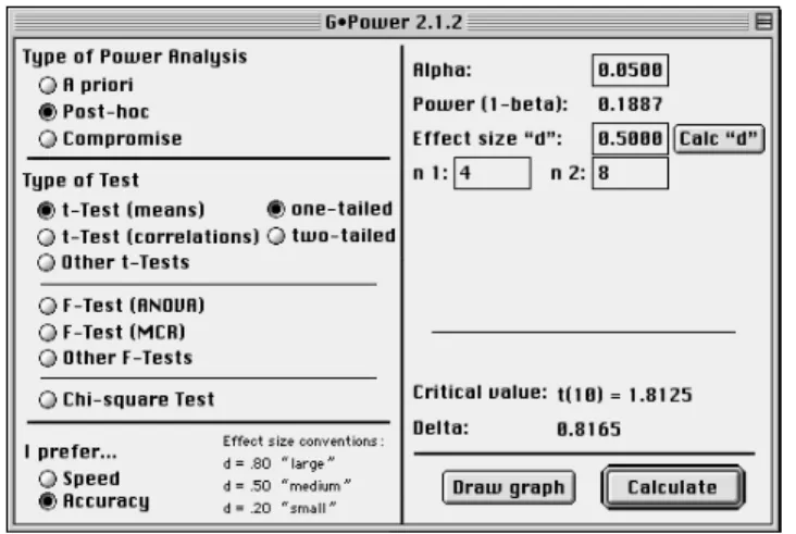
Figure 1: GPower display of a post-hoc power analysis for
a t-test (means) situation. For details see text
.
word‐stem completion task. Relative to controls, amnesic patients completed fewer word stems with words they had seen before. Taking into account that the sample included only 4 amnesics and 8 controls, the statistical power of the t‐
test for independent samples must have been rather small. Additionally, the unequal sample sizes in the two groups tend to reduce statistical power. This is evident when we have a look at the noncentrality parameter δ which defines the noncentral t‐distribution under H1 and reflects the
degree to which H0 is false (Johnson & Kotz, 1970, Chap. 31):
d n n1 2
N
δ= ⋅ ⋅ (1)
with n1 and n2 as the sample sizes of the two groups (amnesics and controls), N = n1 + n2, and d = (μ1 ‐ μ2 ) / σ. The symbol d (commonly called Cohen’s d) is the effect size
index for independent samples t‐tests used by Cohen (1988).
μ1 and μ2 are the population means of the two groups. For
standardization purposes, the difference of population means is divided by the common standard deviation of the two populations, σ. H0 of the one‐tailed t‐test assumes μ2 ‐ μ1
≤ 0, H1 assumes μ2 ‐ μ1 > 0. For a specified total sample size
and a given d, Equation (1) shows that the more unequal the
group sizes, the smaller δ will be, and with it, the smaller will be the statistical power.3
3
Note that the relationship between the difference of the sample sizes n1 and n2 and power is modulated by the size and the magnitude of disparity of the standard deviations in the two groups that enter into the calculation of Cohen’s d. When the two standard deviations are different in size, power will vary depending on which group (the larger or the smaller) has the larger standard deviation and on the magnitude of this disparity (see e.g. Myers & Well, 1995). For the example chosen here, this complication of affairs is not of any relevance because we assume equality of standard deviations for the two groups (see next paragraph).
But how large was the statistical power for the reported results of Warrington and Weiskrantz (1970) in the word‐ stem completion task, if we assume that the underlying population means equalled 14.5 for the amnesic patient group and 16 for the control group? Let us assume that the standard deviation of test performance equalled 3 in the underlying populations of each group (unfortunately, neither the standard deviation of the samples nor the empirical t‐values have been reported). In GPower we have
to choose «Post‐hoc» as type of power analysis and «t‐Test
(means)» as type of test (see Figure 1). Because the hypothesis is directional—we want to know whether controls are better than amnesics—a «one‐tailed» test is selected. Next, we determine with «Calc “d”» d = (16 –
14.5)/3 = 0.5 as the size of the effect to be detected. An effect of this size equals “medium” effects in terms of Cohen’s (1988) conventions. What was the probability to find this effect given a level of α = .05? We specify α = .05, n1 = 4, and
n2 = 8. The result is disillusioning. The statistical power of this test amounts to only .1887. GPower also returns the
critical t‐value associated with the chosen α level, that is, t(10) = 1.8125, and the noncentrality parameter δ = 0.8165
determined by sample size and specified effect size d (see
Equation 1).
Conclusion: There was hardly any chance to detect a medium sized deficit of amnesics in Warrington and Weiskrantz’ (1970) word‐stem completion task. We can use the «Post‐hoc» type of power analysis to determine of what size the performance difference between groups in the word‐stem completion task necessarily would have been to find this difference with a statistical power of .95. To this end, we have to keep the program inputs as specified above (α, n1, n2), but increase the effect size “d” until the calculated statistical power reaches .95. This happens with an effect size of d = 2.1694. This standardized effect size value of
= (μ1 ‐ μ2) / σ into (μ1 ‐ μ2) = d ×σ and by inserting the values
of the example, 2.1694 × 3 = 6.5082). This result implies that a population mean difference not less than 6.5082 words in favor of the control group would have been necessary to achieve a power of .95.
Alternatively, if we want to detect an effect of size d = 0.5
with n1 = 4, n2 = 8, and equally large α and β error probabilities (q = 1), the «Compromise» option has to be
chosen as type of power analysis (see Figure 2). Here, we specify the «Beta/alpha ratio» as “1” if we consider both types of error as equally serious.4
Then GPower returns α = β
= .3422 (associated with a critical value of t(10) = 0.4186).
Under the prevailing circumstances, choosing this significance level is the best possible decision. However, this statistical test is hardly any better than tossing a coin to decide whether to accept or reject H0.
Paired samples t‐test
In succession of Gesell and Thompson’s (1929) work, a number of experiments with monozygotic pairs of twins have been conducted giving one randomly chosen twin training of specific motor skills while the other one did not obtain any training program. This allowed for a controlled investigation of whether certain abilities (e.g. learning to walk, control of the bladder) develop in a process of maturation or whether environmental influences can promote or impair this development.
Imagine that we want to replicate such a twin study which shall be analyzed with a paired samples t‐test. Let us
further assume that there is only a pool of 20 pairs of twins available. What are reasonable error probabilities we have to accept for our statistical test?
X and Y denote the age at which the trained and the
untrained twin, respectively, will master a special motor ability. H0 of the one‐tailed paired samples t‐test is
characterized by x‐y = x ‐ y ≤ 0, with x‐y denoting the
population mean of the age differences of each twin pair. The effect size dz is defined as:
2 2 2cov 2 2 2
x y x y x y
z
x y x y xy x y x y
d μ μ μ
σ σ σ σ σ
− − −
−
= = =
+ − + − ρσ σ
, (2)
with σx‐y being the standard deviation of the (X – Y)
differences, covxy being the covariance, and ρ being the
(positive) correlation between the X and Y values in the
population given H1 is true. Other things being equal, the
larger the correlation ρ, the smaller the denominator will be, and the larger will be the effect size index dz. If H1 is true,
4
Alternatively, values of q > 1 could be used if a type‐2 error is considered less serious than a type‐1 error.
the distribution of our test statistic is the noncentral t‐
distribution with N – 1 degress of freedom (N denotes the
number of twin pairs, i.e. the measurement pairs) and a noncentrality parameter
x y z
x y
N d N
μ δ
σ −
−
= ⋅ = ⋅ . (3)
Let us assume that on average the developmental difference in a specific motor skill amounts to 2 months. For a specific motor skill, the standard deviation of the age difference may amount to 4 months. Hence, following Equation (2), the effect size to be detected with this replication study equals dz = 2/4 = 0.5. Because we want to decide upon the size of the α and β error probabilities given N and dz are fixed, we need the «Compromise» analysis in GPower. The option «t‐Test
(means)» we have used in the previous example is based on
independent samples and calculates the degrees of freedom
as N – 2. This is no longer adequate for the current situation
because the twin data are dependent. For a paired samples t‐
test there are N – 1 degrees of freedom. Therefore, we have
to choose the option «Other t‐Tests» for which the degrees of freedom can be determined independently of N. The
hypothesis is directional again—we want to know whether trained twins are beyond their untrained siblings in their motor skill development—so that we choose the «one‐ tailed» option. In «Other t‐Tests», the to‐be‐specified effect size is labelled f instead of d.5 The noncentrality parameter is calculated as follows:
δ= ⋅f N. (4)
Comparing Equations (3) and (4) we see that the calculated
dz value (i.e. 0.5) can be inserted for the effect size f to obtain
the correct noncentrality parameter for matched‐pairs t‐tests
using the «Other t‐Tests» option. «N» has to be set to 20 (20
pairs of twins were available). If α and β shall be of same size, the »Beta/alpha ratio» option again has to be set to “1”. The test has N – 1 = 19 degrees of freedom («DF for t‐Test»). GPower returns a noncentrality parameter of δ = 2.2361 and
recommends to choose α = β = .1357. For this situation the power is 1 ‐ β = .8643. In order to reject H0 (i.e., in order to reject the hypothesis of no differences between the twins, which implies rejecting the maturation hypothesis) and to accept the H1 (i.e., to accept the “environmental influences” hypothesis), the empirical t‐value has to exceed the critical
value t(19) = 1.1328. Even though this result is less
devastating than that of the previous example, there is nevertheless a large error probability associated with each
5
The reason for using the symbol f rather than d is that the «Other t‐ Tests» option of GPower has been designed to provide power analyses for any type of t‐test, not just t‐tests for means.
decision possible. In order to reduce this error probability, the sample size would have to be increased. To what extend we would have to increase the sample size can be incrementally determined with the «Post‐hoc» analysis option. A «Post‐hoc» analysis again with the options «Other t‐Tests» and «one‐tailed» as well as the specifications α = .05,
f = 0.5, N = 45, and df = 44 returns a power value of 1 ‐ β =
.9512. A sample of this size is necessary to obtain a power level above .95.
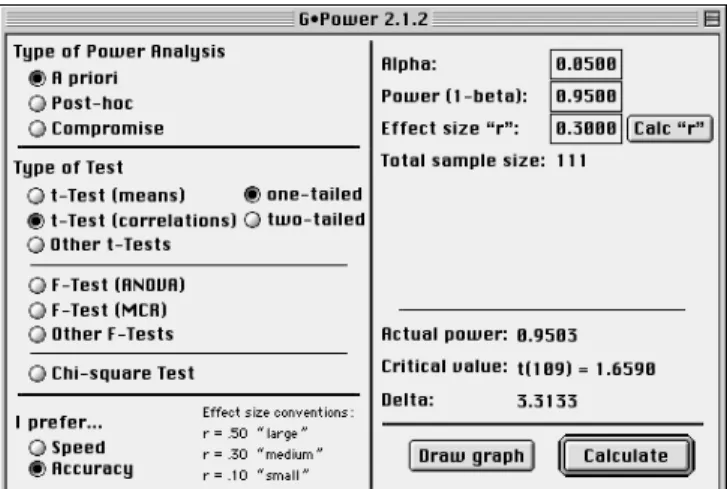
Figure 3: GPower display of an a priori power analysis for a t-test
(correlations) situation. For details see text. In the above example, pairs of twins provided the
dependent data. As a matter of course, we would have to proceed analogously for other kinds of dependent data, for example, for repeated measurements of the same subjects.
t‐test for correlations6
Berry and Broadbent (1984) investigated the relation between task performance in controlling a computer simulation and verbalizable knowledge about the simulated system. Experiment 1 found a negative correlation (in the range of ‐.25 and ‐.30) between both variables. The better the participants controlled the simulation, the worse they were able to provide information about the simulated system.
However, this negative correlation was not statistically significant. The authors attributed the lack of significance to the small sample size (N = 12). But how large was the
probability to find a correlation of a specified size in this study?
Have a look at the definition of the noncentrality parameter δ for t‐tests for correlations between two
variables:
22
1 N
ρ δ
ρ
= ⋅
− , (5)
with ρ as the population correlation associated with H1, and N as the sample size—that is the number of measurement
pairs. According to Cohen (1988) correlations of ρ = .30 are defined as medium sized effects. What are the odds to find an effect of this size in an experiment like the one described by Berry and Broadbent (1984)? We have to choose «Post‐
6
We would like to thank Dave Kenny for making us aware of the fact that the t‐test (correlations) power analyses of GPower are correct only in the point‐biserial case (i.e., correlations between a binary variable and continuous variable, the latter being normally distributed for each value of the binary variable). For correlations between two continuous variables following a bivariate normal distribution, the t‐test (correlations) procedure slightly overestimates power. The procedures for correlations available in GPower 3 provide an exact solution to this problem (Faul et al., 2007).
hoc» as type of power analysis and «t‐Test (correlations)» as type of test. The test is «one‐tailed» because we want to test
H0: ρ ≥ 0 versus H1: ρ < 0. Enter r = .30 as effect size measure, N = 12 as sample size, and α = .05. The noncentrality
parameter turns out to be δ = 1.0894, a t‐value of t(10) = ‐
1.8125 or below denotes a significant result. However, statistical power is only 1 ‐ β = .2648. Berry and Broadbent’s (1984) explanation for not finding a significant correlation seems to be very plausible: their study lacked statistical power. But how large should the sample be in order to find medium effects with a power of .95? Change the settings to «A priori» type of analysis, enter .05 as α, .95 as power, and .30 as effect size r (see Figure 3). The required sample size
amounts to N = 111. The critical t‐value equals t(109) = ‐
1.6590, the noncentrality parameter is δ = 3.3133.
Power analyses for F‐tests
We will restrict our descriptions to power analyses for analyses of variance for fixed effects. These analyses can be conducted with the «F‐Test (ANOVA)» option. We will describe neither the «F‐Test (MCR)» option (for F‐tests in
multiple regression/correlation analyses) nor the «Other F‐ Tests» option (for approximate F‐tests for fixed factors in
mixed models and approximate multivariate analysis of variance (MANOVA) F‐tests).
The effect size index of relevance is the index f or f2. The
relation between f2 and the noncentrality parameter of the
noncentral F‐distribution is given by:
2 2
f n k f N
λ= ⋅ ⋅ = ⋅ , (6)
with n denoting the number of subjects in each of the k
groups. The effect size index f is defined as:
22
1
f η
η
=
− , (7)
with η2 as the amount of the total population variance
explained by the group differences specified in H1. In case of
calculated as follows:
2
1 ( )
k
j j
j n
N f
μ μ
σ
= ⋅ −
=
∑
. (8)
In Equation (8), nj denotes the number of subjects, j the
population mean of group j,
1
( kj nj j) N
μ μ
=
=
∑
⋅ / theweighted mean of the k population means, N the total
sample size, and σ the population standard deviation in each group.
One‐factorial designs
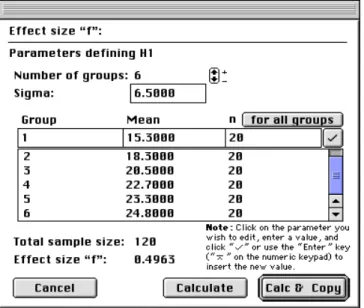
Consider a study on anger expression by Schmitt, Hoser, and Schwenkmezger (1991). The authors investigated whether the anger expressed in response to damage caused by another person depends on the perpetrators’s degree of responsibility for this damage. The degree of responsibility was manipulated in six conditions. Let us assume that we want to replicate the study by Schmitt et al. (1991). H0
implies that the six groups do not differ in the degree of anger expressed. We will base the population effect size estimation for our fictitious example on the empirical effect that was found in the study at hand. GPower allows to
calculate this effect by first choosing «F‐Test (ANOVA)» as type of test (irrespective of all other settings) and then by clicking on the «Calc “f”» button. A new window appears (see Figure 4). Change the «Number of groups» to 6. By inserting the group sample sizes (20), the group means of the measured degrees of expressed anger (that is 15.3, 18.3, 20.5, 22.7, 23.3, and 24.8, cf. Schmitt et al., 1991, p. 641), and their average standard deviation «Sigma» (≈ 6.5; M. Schmitt, personal communication, April 1995), we obtain f = 0.4963.
How many subjects would be necessary in the replication
study if we were willing to accept α = β = .05? In GPower,
choose «A priori» as type of analysis and «F‐Test (ANOVA)» as type of test with the option «Global»7
. Set α = .05, 1 ‐ β = .95, f = 0.4963, and number of groups to 6. The
noncentrality parameter equals 22.1682, the critical F‐value
is F(5, 84)= 2.3231. We will need N = 90 participants⎯that is
15 in each group⎯for this replication.
Figure 4: GPower effect size computation of f based on
the empirical data. For details see text.
Multi‐factorial designs
Koele (1982) exemplifies statistical power analyses for complex designs. Assume an A × B design with fixed‐effects
variables. Factor A comprises kA = 3, factor B comprises kB =
4 levels. What is the statistical power for the tests of the two main effects as well as for that of the interaction? The procedure is similar to the one‐factorial case described in the paragraph above. However, the number of denominator degrees of freedom is reduced by the additional variables (i.e., N ‐ kA × kB). To follow Koele’s (1982) examples, we
choose «Post hoc» as type of analysis in GPower, «F‐Test
(ANOVA)» as type of test including the option «Special», and α = .05. Koele (1982) defines f2 = 0.05; accordingly we
specify f = 0.05= 0.2236 in GPower. Following Koele’s
example, there are 10 observations in each of the 12 cells of the experimental design. Thus, the total sample size N has to
be set to 120. The number of cells (12) has to be inserted into the «Groups» option. To calculate the statistical power for factor A, we need to know the numerator degrees of
freedom for this factor, that is, kA ‐ 1 = 2. Insert this
information into «Numerator df». GPower returns λ = 5.9996,
a critical F‐value of F(2, 108) = 3.0804, and a statistical power
of 1 ‐ β = .5714. Correspondingly, power can be calculated for factor B by changing the numerator degrees of freedom
to kB ‐ 1 = 3. For this case, power is not more than .5020, the
critical F value equals F(3, 108) = 2.6887. Even worse,
statistical power drops to .3806 with a critical value of F(6,
108) = 2.1837 when we are interested in the interaction of factors A and B with (kA – 1)( kB – 1) = 6 numerator degrees
of freedom.
The small disparities between the GPower results and the
values reported by Koele (1982) are due to computational differences. Whereas Koele’s results are based on approximations, exact routines are used in GPower to
calculate the relevant distributions (for details, see Erdfelder et al., 1996). Note that there may be larger differences between GPower results and the results obtained by
7
Figure 5: GPower effect size computation of ω based on the therapy success rates under H0 and H1. For details see text
.
Table 1. Cell probabilities in the 2 × 2 contingency table under the H1 with type of therapy and therapy success as row and column variables, respectively.
Therapy success
Success Failure
Σ
X .88 × .5 = .440 .12 × .5 = .060 .500 Type of
therapy
Y .79 × .5 = .395 .21 × .5 = .105 .500
Σ
.835 .165 1.000following Cohen’s (1988) suggestions to calculate statistical power for complex designs. Evidence has been provided that Cohen’s power assessment procedure for interaction tests is flawed (Bradley, Russell, & Reeve, 1996; Erdfelder et al., 1996; Koele, 1982, footnote 1).
Power analyses for χ2‐tests
Two types of χ2‐tests are commonly applied in
psychological research (cf. Cohen, 1988): (a) contingency tests (also called independence tests) assessing deviations (H1) from stochastic independence (H0) of two or more
categorical variables and (b) goodness‐of‐fit tests of a theoretical distribution to frequency data. Statistical power computations are based on the noncentral χ2‐distribution for
both cases (Johnson & Kotz, 1970, Chap. 28). Its noncentrality parameter
λ ϖ= 2⋅N (9)
is the product of the sample size N and the squared effect
size index
1 0 2
0 1
( )
m
i i
i i
p p
p ϖ
=
−
=
∑
. (10)In Equation (10), m denotes the number of categories, p0i the
probability of category i under H0, and p1i the probability of
category i under H1.
Let us have a look at a contingency test of the following type: The success rate of therapy X is quite large with px =
.88. Unfortunately, therapy X is also very expensive. Assume that a new therapy Y would be much cheaper. Of course, this new therapy should only be applied if its success rate is not (significantly) smaller than that of therapy X. This situation corresponds to a test of H0: py ≥ px against H1: py < px which can be tested with a one‐tailed χ2‐
contingency test for 2 × 2 contingency tables. Type of therapy (X vs. Y) functions as the row variable and therapy success (success vs. failure) as the column variable. Half of the sample is assigned to therapy X and Y, respectively. We want to detect a disadvantage of therapy Y given there is
one with a high degree of certainty. In other words, if the statistical test does not reveal a difference between the two therapies, we want to be very sure that there really is no difference. Therefore, statistical power is set to 1 ‐ β = .95. By contrast, we accept a risk of α = .20 to incorrectly rejecting therapy Y as less efficient than X. By definition, we will call therapy Y less efficient than X only if its success rate undershoots the success rate of X by at least .09. With a success rate for therapy X of px = .88, this implies a success
rate for therapy Y of py = .88 ‐ .09 = .79. The H1 cell
probabilities of the 2 × 2 contingency table implied by these specifications are displayed in Table 1.
What sample size N is needed for this test situation? To
answer this question we choose «A priori» as type of analysis and «Chi‐square Test» as type of test. GPower
calculations are based on a nondirectional χ2‐test situation.
For the directional test problem we face, α is set to .40 instead of .20. Power is set to .95. The effect size measure ω which corresponds to the alternative hypothesis specified by
px = .88 and py = .79 can be calculated in GPower with the
«Calc “ω”» option button. A submenu appears (see Figure 5). Because 50% of the sample is treated under X and Y, the cell probabilities of the contingency table under H1 yield
.880 × .5 = .440 and .120 × .5 = .060, respectively, as the success and failure rates with therapy X (see Table 1). Analogously, we obtain .790 × .5 = .395 and .210 × .5 = .105, respectively, as the success and failure rates with therapy Y.
H0 predicts statistical independence of therapy and outcome
submenu the effect size ω is calculated as given in Equation (10). We thus obtain ω = 0.1212. Finally, df = 1 has to be
specified in the main window. The noncentrality parameter equals = 6.1696. The a priori analysis returns a necessary N
of 420 and a critical χ2‐value of χ2(1) = 0.7083. If the χ2‐statistic
exceeded this critical value and the sample success rate of
therapy Y were smaller than that of therapy X, we would accept H1. The new therapy Y would have to be rejected. If
the χ2‐statistic did not exceed this critical value, H0 would be
maintained. The less expensive therapy Y could be used. Note that all computations are approximations because the exact distribution of the χ2‐statistic is only a χ2‐distribution
for the asymptotic case, that is, for N →∞. However, with N
= 420, the deviation from the asymptotic distribution is negligibly small8
.
Conclusion
Statistical power considerations are indispensable for the evaluation of statistical decisions as well as for designing studies. With GPower we introduced an easy to use software
tool that facilitates the implementation of various kinds of power analyses.
This paper was restricted to power analyses of the most frequently used statistical tests. We recommend the work of O’Brian and Muller (1993) as well as of Chartier and Allaire (in press, this issue) to those interested in power analyses for repeated measures designs and for multivariate analysis of variance (MANOVA) F‐tests. Power analyses for these
situations can be accomplished in GPower using the «Other
F‐Tests» option, but care has to be taken to correctly specify the noncentrality parameter. Readers seeking information about power analyses for random‐effect ANOVAs are referred to Koele (1982).
References
Berry, D. C., & Broadbent, D. E. (1984). On the relationship between task performance and associated verbalizable knowledge. The Quarterly Journal of Experimental Psychology A: Human Experimental Psychology, 36A, 209‐
231.
8
A Monte Carlo study with 10.000 random samples—each of sample size N = 420—drawn from the population under H1 resulted in an empirical estimation of statistical power of .9514. This estimation arose when each occurrence in which the test statistic exceeded the critical value of 0.7083 was counted as a rejection of H0. If only the subset of test statistics were counted for which the sample success rate of therapy X was larger than that of therapy Y, power estimation equaled .9509. The results show that the statistical power considerations stay valid for the “one‐tailed” decision rule applied in the above example.
Bradley, D. R., Russell, R. L., & Reeve, C. P. (1996). Statistical power in complex experimental designs. Behavior Research Methods, Instruments, & Computers, 28, 319‐326.
Bredenkamp, J. (1972). Der Signifikanztest in der psychologischen Forschung. Frankfurt a.M.: Akademische
Verlagsgesellschaft.
Bredenka m p, J. (1980). Theorie und Planung psychologischer Experimente. Darmstadt: Steinkopff.
Buchner, A., Erdfelder, E., & Faul, F. (1996). Teststärkeanalysen. In E. Erdfelder, R. Mausfeld, T. Meiser, & G. Rudinger (Eds.), Handbuch quantitative Methoden (pp. 123‐136). Weinheim: Beltz Psychologie‐
Verl.‐Union.
Chartier, S., & Allaire, J.‐F. (in press). Power estimation in multivariate analysis of variance. Tutorials in Quantitative Methods for Psychology.
Cohen, J. (1988). Statistical power analysis for the behavioral sciences (2nd ed.). Hillsdale, NJ: Lawrence Erlbaum
Associates.
Erdfelder, E. (1984). Zur Bedeutung und Kontrolle des beta‐ Fehlers bei der inferenzstatistischen Prüfung log‐linearer Modelle. Zeitschrift für Sozialpsychologie, 15, 18‐32.
Erdfelder, E., Buchner, A., Faul, F., & Brandt, M. (2004). GPOWER: Teststärkeanalysen leicht gemacht. In E. Erdfelder & J. Funke (Eds.), Allgemeine Psychologie und deduktivistische Methodologie (pp. 148‐166). Göttingen:
Vandenhoeck & Ruprecht.
Erdfelder, E., Faul, F., & Buchner, A. (1996). GPOWER: A general power analysis program. Behavior Research Methods, Instruments, & Computers, 28, 1‐11.
Faul, F., Erdfelder, E., Lang, A.‐G., & Buchner, A. (2007). G*Power 3: A flexible statistical power analysis program for the social, behavioral, and biomedical sciences.
Behavior Research Methods, 39, 175‐91.
Gesell, A., & Thompson, H. (1929). Learning and growth in identical infant twins. Genetic Psychology Monographs, 6,
1‐123.
Johnson, N. L., & Kotz, S. (Eds.). (1970). Discrete distributions: Distributions in statistics ‐ 2. New York: Wiley.
Koele, P. (1982). Calculating power in analysis of variance.
Psychological Bulletin, 92, 513‐516.
Myers, J. L., & Well, A. D. (1995). Research design and statistical analysis. Mahwah, N.J.: Erlbaum.
OʹBrien, R. G., & Muller, K. E. (1993). Unified power analysis for t‐tests through multivariate hypotheses. In L. K. Edwards (Ed.), Applied analysis of variance in behavioral science (pp. 297‐344). New York, NY, US:
Marcel Dekker.
Schmitt, M., Hoser, K., & Schwenkmezger, P. (1991). Schadensverantwortlichkeit und Ärger Zeitschrift für Experimentelle und Angewandte Psychologie, 38, 634‐647.
syndrome: Consolidation or retrieval? Nature, 228, 628‐
630.
Manuscript received December 20th, 2006
Manuscript accepted October 31st, 2007