On Signal Restoration by Piecewise Monotonic
Data Approximation
I. C. Demetriou and V. Koutoulidis
Abstract—We consider the application of the piecewise monotonic data approximation method to some problems that are derived from univariate signal restoration. We present numerical examples in order to show the efficacy of a software package that implements the method in data fitting and in denoising data from a medical image. The piecewise monotonic approximation method makes the smallest change to the data such that the first differences of the smoothed data change sign a prescribed number of times. Our results exhibit some strengths and certain advantages of the method over wavelets and splines. Therefore, they may be helpful to the development of new algorithms that are particularly suitable for MRI and CT calculations.
Index Terms—data smoothing, divided differences, magnetic resonance imaging, piecewise monotonic approximation, signal restoration
I. INTRODUCTION
P
iecewise monotonic data approximation introduced by Demetriou and Powell [6]. Since then some useful applications of the method in signal restoration, image processing and spectroscopy have been appeared (see, for example, [12], [19], [2] and references therein). Let{φ(xi) :i = 1,2, . . . , n} be a sequence of values of a signal φ(x)
measured at the abscissae x1 < x2 < · · · < xn, but these measurements include errors (noise) and the data are to be used to provide a restoration to φ(x). We assume that if the signal has turning points, then the number of measurements is substantially greater than the number of turning points. Therefore some algorithms are proposed in [6] that modify the measurements if their first differences {yi+1−yi :i= 1, . . . , n−1} include more than k−1 of sign changes, a condition which allowskmonotonic sections to the smoothed data, kbeing a prescribed integer.
Signals in practice are piecewise monotonic, but in many applications the number of monotonic sections they contain is not known in advance. Prior knowledge about the geometry of the signal may provide good estimates of k, but it is not inefficient to run the algorithm of [6] for a sequence of integersk if a suitable value is not known.
Some advantages of this technique over other currently used smoothing algorithms are as follows. First, there is no need to choose a set of approximating functions. Second, the smoothing process is a projection because, if it is applied to the smoothed data, then no changes are made to. Third, the
Manuscript received April 16, 2013.
This work was supported in part by the University of Athens under Research Grant 11105.
I. C. Demetriou is with the Department of Economics, Univer-sity of Athens, 8 Pesmazoglou street, Athens 10559, Greece (e-mail: [email protected]).
V. Koutoulidis is with the 1st Department of Radiology, Medical School, University of Athens, Aretaieion Hospital, 76 Vas. Sophias Ave., Athens 11528, Greece (e-mail: [email protected]).
technique is particularly suitable when the errors are large and uncorrelated.
Weaver [19], with respect to the use of monotonicity algorithms in fMRI, points out that the primary advantage of the monotonic increasing approximation is that it smooths the data as little as possible without blurring the edges; it leaves increases unchanged; both sharp and smooth increases remain unchanged, so no smoothing occurs at all; it avoids Gibb’s ringing. Analogously for the monotonic decreasing approximation. Lu [12] has combined the Tikhonov regu-larization [18] with the piecewise monotonicity criterion in an iterative scheme for signal restoration. In this way, the piecewise monotonicity criterion not only is different from a low-pass filter, which is actually subjected to the Gibbs effect, but also very efficient in signal denoising. As general references in signal and image processing see [14] and [9].
The paper is organized as follows. In Section II we outline the method for piecewise monotonic data approximation. In Section III we consider numerical examples that illustrate the method on data from a periodic function with simulated errors and data from a noisy medical image. The results are instructively analyzed and the smoothing capability of the method is demonstrated. In Section IV we present some concluding remarks and discuss on the possibility of future directions of this research.
In order to apply the piecewise monotonicity method to a sequence of data, only one parameter, namely k, must be set by the user. Then the method automatically and simultaneously obtains the optimal turning points and the best fit. Some Fortran software, namely L2WPMA, that implements the method was written by one of the authors [5] that is suitable for processing large numbers of data in real time. It calculates efficiently a global solution in quadratic complexity with respect ton, a complexity which reduces to only O(n) when k = 1 or k = 2. At the end of the calculation a spline representation of the solution and the corresponding Lagrange multipliers are provided. The software package has been tested on a variety of data sets showing a performance that does provide in practice shorter computation times than the complexity indicates in theory.
II. PIECEWISEMONOTONICDATAAPPROXIMATION
We regard the measurements as components{φi=φ(xi) :
i= 1,2, . . . , n}of an−vectorφ. We assume for the moment thatk is known and the method of [6] calculates a vectory
that minimizes the sum of the squares
Φ(y) =
n
X
i=1
subject to the piecewise monotonicity constraints
ytj−1 ≤ytj−1+1≤ · · · ≤ytj, if j is odd ytj−1 ≥ytj−1+1≥ · · · ≥ytj, if j is even
)
, (2)
where the integers {tj : j = 0,1, . . . , k}, specifically the positions of the turning points or extrema of the fit, satisfy the conditions
1 =t0≤t1≤ · · · ≤tk=n. (3)
The integers {tj : j = 1,2, . . . , k−1} are not known initially and they are variables in the optimization calculation that gives a best fit. This raises the number of combinations of integer variables to the formidable order O(nk)
, but fortunately the piecewise monotonic approximation problem is characterized by the following properties that allow an efficient and automatic calculation of an optimal fity: (a) The constraints prevent the equationy=φfrom holding, because ifφdoes not satisfy the piecewise monotonicity constraints, then {tj :j = 1,2, . . . , k−1} are all different. (b) At the turning points of a best fit y, the interpolation conditions
ytj =φtj, j= 1,2, . . . , k−1 (4)
hold. (c) Each monotonic section in a best piecewise mono-tonic fit is the optimal fit itself to the corresponding data, so it can be obtained by a separate calculation. Indeed, the components {yi:i=tj−1, tj−1+ 1, . . . , tj} on[xtj−1, xtj]
minimize the sum of the squares
tj X
i=tj−1
(yi−φi)2 (5)
subject to the constraints
yi≤yi+1, i=tj−1, . . . , tj−1, if j is odd (6)
or subject to the constraints
yi≥yi+1, i=tj−1, . . . , tj−1, ifj is even. (7)
In the former case the sequence {yi : i = tj−1, tj−1 + 1, . . . , tj} is the best monotonic increasing fit to {φi :
i = tj−1, tj−1 + 1, . . . , tj} and on the latter case the
best monotonic decreasing one. Therefore, provided that {ti :i = 1,2, . . . , k−1} are known, the components of y can be generated by solving a separate monotonic problem on each section[xtj−1, xtj]. The problem with the decreasing
monotonicity may be treated computationally as the problem with the increasing monotonicity after reversing the order of the data. It is important to note that the constraints on y
are linear and have linearly independent normals. Also, the second derivative matrix with respect to y of the objective function (5) is twice the unit matrix. Thus, the problem of minimizing (5) subject to (6) is a strictly convex quadratic programming problem that has a unique solution (see [8] for a general reference in optimization). The calculation of a best monotonically increasing approximation toφseeks intervals where its components have different constant values. The intervals are formed by using the remarkable property that any constraints which are satisfied as equalities by the best approximation subject to a subset of the monotonicity constraints are also satisfied as equalities by the best approx-imation subject to all monotonicity constraints. Algorithm
1 of [6] performs the calculation of the best monotonic increasing fit on[xtj−1, xtj]together with all the numbers
ℓ
X
i=tj−1
(yi−φi)2, ℓ=tj−1, . . . , tj (8)
in onlyO(tj−tj−1)computer operations. This surprisingly little work contributes heavily to the efficiency of the calcu-lation of an optimal piecewise monotonic fit. Note that the monotonic problem has raised an extensive interest due to its applications in economics, operations research, decision analysis, non-parametric regression and data analysis (see, for example, [15] and references within). (d) The optimal integer variables when the calculation is solved for two values ofkthat differ by 2 have an interlacing property. The local maxima of a best approximation withk−2sections are separated by the local maxima of a best approximation with
ksections and similarly for the local minima. This property provides a substantial improvement in the efficiency of the method.
Further, it is proved that an optimal fity associated with the integer variables {tj : j = 1,2, . . . , k−1} can split at
tk−1into two optimal sections. One section that provides an
optimal fit on[x1, xtk−1], which in fact is similar toy with
one monotonic section less, and one section on [xtk−1, xn]
that is a single optimal monotonic fit to the remaining data. Hence the optimization problem is amenable to dynamic programming, where the positions of the turning points of the required fit are also variables of the calculation. The implementation of this idea includes several options that are considered by [6] and [4], and still there is room for further research. Demetriou [5] especially implements an algorithm of [4] and provides a versatile Fortran package that derives a solution in only O(nm +km2)
computer operations, where m is the number of local extrema of the data. Here, for example,pis the index of a local maximum of the sequence φi, i = 2, . . . , n −1 if φp−1 < φp and
φp> φp+1. Furthermore, the reported numerical results are
by far better than this complexity, which makes piecewise monotonic approximation very efficient in practice.
The method may also be applied to the problem where inequalities (2) are replaced by the reversed ones, in which case the first section of the fit is decreasing. The latter problem may be treated computationally as the former one after an overall change of sign ofφ. Is not inefficient to run the method with both options, if the user opts for letting the method decide whether the first section is increasing or decreasing.
Some serious applications of the piecewise monotonic approximation approach in medical practice related with noise reduction in magnetic resonance imaging and in signal reconstruction were reported by [19] and [12] at time prior to [5]. Specifically, [19] first makes use of a Fourier filter in order to select significant extrema and then constrains the data to be monotonic between extrema.
III. NUMERICALEXAMPLES INSIGNALRESTORATION WITHPIECEWISEMONOTONICITYCONSTRAINTS
To illustrate the efficacy of the method in signal restoration we present two numerical examples. The first example is a best fit with k = 6 monotonic sections to n = 100
measurements of the function
φ(x) =sin(5x)−x (9)
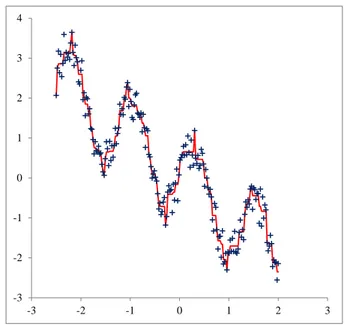
at equally spaced abscissae on the interval [−2.5,2]. The measurements were generated by adding uniformly dis-tributed random numbers from the interval(−0.5,0.5)to the function valuesφ(xi), i= 1,2, . . . , n. The data are presented in the second and the third column of Table I, although the abscissae are irrelevant to this calculation. Without any preliminary analysis the data were fed to L2WPMA, 6 mono-tonic sections were required and the solution was reached immediately in a common pc. The best fit is presented in the fourth column of Table I and the corresponding Lagrange multipliers are presented in the fifth column; the horizontal lines indicate the turning point positions. Fig. 1 shows the data and the fit; the data are denoted by (+), the best approximation by (o) and the piecewise linear interpolant to the smoothed values illustrates the fit.
The Lagrange multipliers, one multiplier for each con-straint, are also irrelevant to the actual calculation of the best fit; they are provided because they are useful to further analysis. Indeed, we can immediately notice the correspon-dence between the zero Lagrange multipliers and the inactive constraints. For example, the constraint y2 ≤ y3 is amply satisfied because y2 = 2.839 and y3 = 3.066, while λ2 is zero. The nonzero Lagrange multipliers correspond to active constraints. For example, the equations y3 = y4 = y5 = y6 = y7 = 3.066 (see column 4) are associated with the Lagrange multipliers λ4 = 0.546, λ5 = 0.118, λ6 = 0.651
andλ7= 0.049(see column 5). A sensitivity analysis would conclude that the best fit is strongly dependent upon the placement of all active constraints, because the associated Lagrange multipliers are away from zero. In addition, the inactive constraints allow for freedom in order to follow the data trends. Since a Lagrange multiplier may be interpreted as a number measuring the marginal potential change in the value of the objective function (1), a relaxation of the corresponding constraint reduces the value of (1) approxi-mately by an amount equal to the magnitude of the multiplier. Therefore, the large moduli of Lagrange multipliers (see, for example, λ28 = −10.628, λ29 = −10.429, etc) on the long range [x17, x39] of constant components suggest that substantial improvements may be possible if we increase
k by 2. Thus, if we assume that the best fit with k+ 2
monotonic sections is as good as the best fit withksections, whilek+2sections are allowed, then replacing, for example,
y28 by φ28 retains feasibility because y27 < y28 and
y28> y29, and reduces the objective function by the amount
(φ28−y28)2
. The remark suggests that there is room for improving the fit by increasing k, while the magnitudes of the Lagrange multipliers indicate the range [x17, x39] as a range for potential improvement of the fit.
The first attempt at fitting the data, on the purpose of demonstrating some features of the piecewise monotonic fit, was not entirely satisfactory. Indeed, the turning points of the fit are at the abscissae x8, x50, x64, x78 and x89, satisfying
-4 -3 -2 -1 0 1 2 3 4
-3 -2 -1 0 1 2 3
Fig. 1. Graphical representation of the data given in Table I. The data of column 2 annotate the x-axis. The data of column 3 are denoted by (+) and the best fit of column 4 by (o). The solid line illustrates the fit.
-3 -2 -1 0 1 2 3 4
-3 -2 -1 0 1 2 3
Fig. 2. Best fit (solid line) with k= 8monotonic sections ton= 200 measurements (+) of function (9) produced as described in Section III.
in addition the interpolation conditions (4). Notice also that the monotonic algorithm averages any data values that are needed to achieve monotonicity. For example, y3 = y4 = y5 = y6 = y7 = (P7
i=3(φi))/5 = 3.066, while the
TABLE I
BEST FITS WITHk= 6ANDk= 8MONOTONIC SECTIONS TO MEASUREMENTS OF FUNCTION(9)
Best Fit k=6 Best Fit k=8 Best Fit k=6 Best Fit k=8
xi φi yi λi yi λi xi φi yi λi yi λi
1 –2.50 2.066 2.066 2.066 51 –0.23 –0.710 –0.855 0.000 –0.855 0.000
2 –2.45 2.839 2.839 0.000 2.839 0.000 52 –0.18 –0.999 –0.855 0.289 –0.855 0.289
3 –2.41 3.339 3.066 0.000 3.066 0.000 53 –0.14 –0.678 –0.678 0.000 –0.678 0.000
4 –2.36 2.852 3.066 0.546 3.066 0.546 54 –0.09 –0.186 –0.340 0.000 –0.340 0.000
5 –2.32 3.333 3.066 0.118 3.066 0.118 55 –0.05 –0.494 –0.340 0.308 –0.340 0.308
6 –2.27 2.765 3.066 0.651 3.066 0.651 56 0.00 –0.146 –0.146 0.000 –0.146 0.000
7 –2.23 3.042 3.066 0.049 3.066 0.049 57 0.05 0.086 0.086 0.000 0.086 0.000
8 –2.18 3.673 3.673 0.000 3.673 0.000 58 0.09 0.756 0.659 0.000 0.659 0.000
9 –2.14 2.884 2.899 0.000 2.899 0.000 59 0.14 0.561 0.659 0.195 0.659 0.195
10 –2.09 2.914 2.899 –0.030 2.899 –0.030 60 0.18 0.735 0.659 0.000 0.659 0.000
11 –2.05 2.584 2.584 0.000 2.584 0.000 61 0.23 0.583 0.659 0.152 0.659 0.152
12 –2.00 2.442 2.442 0.000 2.442 0.000 62 0.27 0.974 0.908 0.000 0.908 0.000
13 –1.95 2.046 2.157 0.000 2.157 0.000 63 0.32 0.843 0.908 0.132 0.908 0.132
14 –1.91 2.203 2.157 –0.221 2.157 –0.221 64 0.36 1.020 1.020 0.000 1.020 0.000
15 –1.86 2.221 2.157 –0.128 2.157 –0.128 65 0.41 0.960 0.960 0.000 0.960 0.000
16 –1.82 1.491 1.491 0.000 1.491 0.000 66 0.45 0.161 0.261 0.000 0.261 0.000
17 –1.77 0.962 1.198 0.000 1.136 0.000 67 0.50 0.362 0.261 –0.200 0.261 –0.200
18 –1.73 1.311 1.198 –0.472 1.136 –0.348 68 0.55 –0.195 –0.195 0.000 –0.195 0.000
19 –1.68 0.886 1.198 –0.247 0.886 0.000 69 0.59 –0.848 –0.848 0.000 –0.848 0.000
20 –1.64 0.728 1.198 –0.870 0.728 0.000 70 0.64 –1.157 –1.057 0.000 –1.057 0.000
21 –1.59 0.227 1.198 –1.810 0.227 0.000 71 0.68 –1.025 –1.057 –0.200 –1.057 –0.200
22 –1.55 0.236 1.198 –3.752 0.236 0.000 72 0.73 –0.989 –1.057 –0.136 –1.057 –0.136
23 –1.50 0.700 1.198 –5.677 0.700 0.000 73 0.77 –1.127 –1.127 0.000 –1.127 0.000
24 –1.45 1.114 1.198 –6.674 0.704 0.000 74 0.82 –1.753 –1.753 0.000 –1.753 0.000
25 –1.41 0.369 1.198 –6.842 0.704 0.820 75 0.86 –1.855 –1.855 0.000 –1.855 0.000
26 –1.36 0.805 1.198 –8.500 0.704 0.151 76 0.91 –1.951 –1.876 0.000 –1.876 0.000
27 –1.32 0.527 1.198 –9.285 0.704 0.354 77 0.95 –1.801 –1.876 –0.151 –1.876 –0.151
28 –1.27 1.297 1.198 –10.628 1.297 0.000 78 1.00 –2.169 –2.169 0.000 –2.169 0.000
29 –1.23 1.576 1.198 –10.429 1.542 0.000 79 1.05 –1.574 –1.739 0.000 –1.739 0.000
30 –1.18 1.507 1.198 –9.673 1.542 0.069 80 1.09 –1.703 –1.739 0.329 –1.739 0.329
31 –1.14 1.924 1.198 –9.054 1.924 0.000 81 1.14 –1.939 –1.739 0.400 –1.739 0.400
32 –1.09 1.680 1.198 –7.601 1.777 0.000 82 1.18 –1.185 –1.185 0.000 –1.185 0.000
33 –1.05 1.874 1.198 –6.637 1.777 –0.194 83 1.23 –0.926 –1.064 0.000 –1.064 0.000
34 –1.00 1.777 1.198 –5.284 1.777 0.000 84 1.27 –1.202 –1.064 0.276 –1.064 0.276
35 –0.95 1.519 1.198 –4.127 1.693 0.000 85 1.32 –0.952 –0.952 0.000 –0.952 0.000
36 –0.91 1.867 1.198 –3.484 1.693 –0.348 86 1.36 –0.899 –0.911 0.000 –0.911 0.000
37 –0.86 1.627 1.198 –2.146 1.627 0.000 87 1.41 –0.922 –0.911 0.022 –0.911 0.022
38 –0.82 1.514 1.198 –1.287 1.520 0.000 88 1.45 –0.594 –0.594 0.000 –0.594 0.000
39 –0.77 1.525 1.198 –0.654 1.520 –0.011 89 1.50 –0.338 –0.338 0.000 –0.338 0.000
40 –0.73 1.150 1.150 0.000 1.150 0.000 90 1.55 –0.376 –0.376 0.000 –0.376 0.000
41 –0.68 0.967 0.967 0.000 0.967 0.000 91 1.59 –0.410 –0.410 0.000 –0.410 0.000
42 –0.64 0.442 0.442 0.000 0.442 0.000 92 1.64 –0.727 –0.727 0.000 –0.727 0.000
43 –0.59 –0.001 –0.001 0.000 –0.001 0.000 93 1.68 –1.166 –1.147 0.000 –1.147 0.000
44 –0.55 –0.343 –0.168 0.000 –0.168 0.000 94 1.73 –1.129 –1.147 –0.037 –1.147 –0.037
45 –0.50 –0.178 –0.168 –0.349 –0.168 –0.349 95 1.77 –1.578 –1.578 0.000 –1.578 0.000
46 –0.45 0.016 –0.168 –0.369 –0.168 –0.369 96 1.82 –1.702 –1.698 0.000 –1.698 0.000
47 –0.41 –0.359 –0.359 0.000 –0.359 0.000 97 1.86 –1.694 –1.698 –0.008 –1.698 –0.008
48 –0.36 –0.949 –0.710 0.000 –0.710 0.000 98 1.91 –1.830 –1.830 0.000 –1.830 0.000
49 –0.32 –0.470 –0.710 –0.479 –0.710 –0.479 99 1.95 –2.773 –2.773 0.000 –2.773 0.000
50 –0.27 –1.035 –1.035 0.000 –1.035 0.000 100 2.00 –2.808 –2.808 0.000 –2.808 0.000
continued
poor fit; all the other turning points remained unchanged. An advantage of having a known underlying function is that we can see whether the fit is more accurate than the measurements and it is. Another feature of the smoothing technique is shown at the rightmost monotonic section of this fit, [x89, x100], where some data errors are too small to be detected by the monotonic constraints. Thus, some data remain unchanged, namelyyi=φi, fori= 90,91,92,98,99 and 100. Further, the particular fit with k = 6 (see Fig. 1) shows that L2WPMA achieves the piecewise monotonicity property it sets out to achieve and, generally, any degree of
undulation in the data can be accommodated by choosing a suitable k. Moreover, we repeated the experiment with
n = 200 data points, but we applied the method of [17],
Athens.
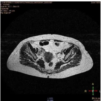
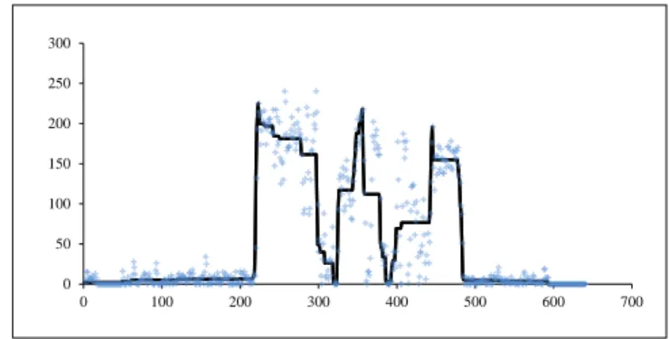
The second example is a fit to 640 data points obtained by the 239th vertical scan line through the640×640gray-scale noisy image in Fig. 3. The pixel intensities are displayed in Fig. 4. The data vary considerably and although exhibit some turning points, reader’s eye is not especially attracted. We seek turning points that might reveal major monotonic trends. The difficulty with these data is that there is no mathematical function that could show the accuracy of any fit. We start by noticing that the total number of local extrema of the data is 126. We fed the data to the computer program of [17] with the data trend test without any preliminary analysis and the resultant fit gave automatically k = 70, thus providing too many turning points. It is likely that the first attempt at estimating suitable turning points of these data is not entirely satisfactory, but this cannot be realized until the fit has been calculated.
Fig. 3. A T2-Weighted Magnetic Resonance Imaging axial slice of the pelvis.
Therefore we carried out some more runs with smaller numbers of turning points, which gives more emphasis to major monotonic trends. The data were fed to L2WPMA and the best fit subject to the piecewise monotonicity constraints with k = 6 was calculated immediately. Fig. 5 displays the data and the fit. The computer program terminated at an optimum with five turning points at the abscissae
0 50 100 150 200 250 300
0 100 200 300 400 500 600 700
Fig. 4. Vertical scan line 239 of the image in Fig. 3. Pixel intensities are denoted by (+).
x223, x322, x356, x389, x445 andx640 and sum of squares of residuals equal to 3355×102
. Indeed the fit to the data is much smoother than are the data values themselves, but we should not forget that the method has revealed the most important k−1 turning points. Thus, in case that the fit might be considered unsatisfactory, we carried out a second run withk= 8, which gave automatically two extra turning points atx361 andx369 by enhancing the fit of Fig. 5 in the interval of adjacent turning points[x356, x389], where the fit seems rather poor. The fit is presented in Fig. 6 and the sum of squares of residuals is reduced to2292×102
. One more run withk= 10, gave two extra turning points atx407 and
x427by enhancing the fit of Fig. 6 in the interval of adjacent turning points[x389, x445]. The fit is presented in Fig. 7 and the sum of squares of residuals is reduced to 1510×102
. In Fig. 5 few noticeable peaks within the range are ignored. The choicesk= 8ork= 10may be satisfactory, in that the associated fit may be an adequate approximation to the data engineer’s best estimate of the truth, revealing turning points and in-between trends that seem to have real significance.
In order not to be misled by the results in usual practices with piecewise monotonic approximation, we mention some ideas that failed to provide optimality. We saw in our examples that all turning points of a best approximation with
k−2 sections were turning points of a best approximation withksections. Also, the extra 2 turning points of the best fit withksections were found in a range of constant components of the best fit withk−2sections. Hence a best approximation with 3 monotonic sections might be obtained by improving the best monotonic approximation after reducing the search for the turning points to ranges of constant components. Nonetheless, the conjecture has been proved not to be true [3]. Moreover, the extra 2 turning points were found to be between adjacent turning points of the best approximation with k −2 sections. However, the turning points of the best approximation withk−2 sections need not be turning points of a best approximation with k sections, because, as was mentioned in Section II, the local maxima of best approximation with k−2 sections are separated (weakly) by the local maxima of best approximation withksections, and similarly for the local minima. Furthermore, if among the Lagrange multipliers there are a few whose magnitudes are much larger than the rest, then simply they anticipate the possibility that more monotonic sections may be needed for obtaining an improved fit.
Piecewise monotonic approximation, in the absence of any structure, requires at least O(m2)
operations when k ≥ 3, because it is necessary to take account of all possible values of (8), forℓ=tj−1, . . . , tj.
low-pass filtering or over the use of basis functions to represent the data, which usually result in ringing and blurring artifacts [12], [19], [11].
0 50 100 150 200 250 300
0 100 200 300 400 500 600 700
Fig. 5. Best fit withk= 6(solid line) to the signal of Fig. 4.
0 50 100 150 200 250 300
0 100 200 300 400 500 600 700
Fig. 6. Best fit withk= 8(solid line) to the signal of Fig. 4.
0 50 100 150 200 250 300
0 100 200 300 400 500 600 700
Fig. 7. Best fit withk= 10(solid line) to the signal of Fig. 4.
IV. CONCLUDINGREMARKS
We have presented applications that show the effectiveness of piecewise monotonic approximation to signal restorations. Piecewise monotonic approximation as a data smoothing approach can have many applications. Despite the large number of local minima that can occur in this optimization calculation, it gives a global solution in quadratic complexity with respect to n, but in practice the complexity is by far lower. The accompanying Fortran software is suitable for calculations that involve several thousand data points and they would be most useful for real time processing applications. In view of the effort that was needed to develop
L2WPMA and certain variants of this package for automating the calculation ofk, it is expected that these packages will be of value to many computer calculations.
Moreover, it would be very helpful to try to solve particular signal processing problems, in order to receive guidance from numerical results and from medical imaging practices [16]. For example, in certain applications in MR spectroscopy we often have good estimates of k [12] that can be utilized by the method of [17]. In addition, one may well combine certain features of our method with wavelets (see, [11], [10]) or other parametric forms (see, for example, splines [1], [7] or semiparametric techniques [20]) if there exists an opportunity for improved practical analyses in medical imaging and computed tomography.
REFERENCES
[1] C. de Boor,A Practical Guide to Splines. Revised Edition, NY: Springer-Verlag, Applied Mathematical Sciences, vol. 27, 2001.
[2] A. P. Bruner, K. Scott, D. Wilson, B. Underhill, T. Lyles, C. Stopka, R. Ballinger and E. A. Geiser, “Automatic Peak Finding of Dynamic Batch Sets of Low SNR In-Vivo Phosphorus NMR Spectra”, unpublished manuscript, Departments of Radiology, Physics, Nuclear and Radio-logical Sciences, Surgery, Mathematics, Medicine, and Exercise and Sport Sciences, University of Florida, and the Veterans Affairs Medical Center, Gainesville, Florida, U. S.
[3] I. C. Demetriou, Data Smoothing by Piecewise Monotonic Divided
Differences, Ph.D. Dissertation, Department of Applied Mathematics
and Theoretical Physiscs, University of Cambridge, Cambridge, 1985. [4] I. C. Demetriou, “Discrete piecewise monotonic approximation by a
strictly convex distance function”, Mathematics of Computation, vol. 64, 209, pp. 157-180, 1995.
[5] I. C. Demetriou, “Algorithm 863: L2WPMA, a Fortran 77 package for weighted least-squares piecewise monotonic data approximation”,ACM
Trans. Math. Softw., vol. 33, 1, pp. 1-19, 2007.
[6] I. C. Demetriou and M. J. D. Powell, “Least squares smoothing of univariate data to achieve piecewise monotonicity”,IMA J. of Numerical
Analysis, vol. 11, pp. 411-432, 1991.
[7] P. Dierckx,Curve and Surface Fitting with Splines, Oxford: Clarendon Press, 1995.
[8] R. Fletcher,Practical Methods of Optimization, Chichester, U. K.: J. Wiley and Sons, 2003.
[9] R. C. Gonzalez and R. E. Woods,Digital Image Processing, 3rd ed. Upper Saddle River, New Jersey: Pearson Prentice Hall, 2008. [10] M. Holschneider, Wavelets. An Analysis Tool, Oxford: Clarendon
Press, 1997.
[11] J. Lu, “On consistent signal reconstruction from wavelet extrema representation”, inWavelet Applications in Signal and Image Processing V, Proc. SPIE, vol. 3169, July 1997.
[12] J. Lu, “Signal restoration with controlled piecewise monotonicity constraint”, Proceedings of the IEEE International Conference on Acoustics, Speech and Signal Processing, 12 May 1998-15 May 1998, Seattle WA, vol. 3, pp. 1621 - 1624, 1998.
[13] M. J. D. Powell, “Curve fitting by splines in one variable”, in
Numerical Approximation to Functions and Data, ed. J. G. Hayes,
The Institute of Mathematics and its Applications, London, U. K.: The Athlone Press, pp. 65 - 83, 1970.
[14] J. G. Proakis and D. G. Manolakis,Digital Signal Processing:
Prin-ciples, Algorithms and Applications, 4th ed. Upper Saddle River, New
Jersey: Prentice Hall, 2006.
[15] T. Robertson, F. T. Wright and R. L. Dykstra, Order Restricted
Statistical Inference, New York: John Wiley and Sons, 1988.
[16] V. M. Runge, W. R. Nitz and S. H. Schmeets,The Physics of Clinical
MR Taught Through Images, 2nd ed. New York: Thieme, 2009.
[17] E. Vassiliou and I. C. Demetriou, “An adaptive algorithm for least squares piecewise monotonic data fitting”,Computational Statistics and
Data Analysis, vol. 49, pp. 591-609, 2005
[18] A. Tikhonov and V. Arsenin,Solution of Ill-Posed Problems, Wash-ington, DC: Winston, 1977.
[19] J. B. Weaver, “Applications of Monotonic Noise Reduction Algorithms in fMRI, Phase Estimation, and Contrast Enhancement”,International
Journal on Innovation, Science and Technology, IJIST, vol. 10, pp.
177-185, 1999.