Tsunami Simulation for Capacity Development

Abstract_{—The 26 December 2004 Andaman mega tsunami} killed about 200, 000 people worldwide. This infamous tsunami serves a potent wakeup call for many countries in the affected regions including Malaysia, Thailand and Indonesia. More recently, the 25 October 2010 tsunami in Mentawai islands of Indonesia that killed more than four hundred people is a recurrent reminder of the hazards of tsunamis in this region. Active research on tsunami simulation and community outreach activities on tsunami education, risk reduction and preparedness are essential to help community develop resilience to tsunamis. Many researchers in the regions have developed their respective long-term programs on tsunami related research for this purpose. Over the past several years, capacity building has been intensely stepped up to develop human resources that are able to perform tsunami simulations for developing inventory of tsunami risk hotspots and evacuation routes. Several international workshops were held in the Indian Ocean and South China Sea regions to propel effective research collaboration. Enlightened by these international workshops, the Malaysian government has appointed the authors to (a) develop tsunami simulation model TUNA, (b) to establish local maps that rank tsunami risk hotspots and their associated characteristics for northwest Peninsular Malaysia and (c) to conduct tsunami modelling workshops for the purpose of developing human resources capable of performing or understanding tsunami simulations in their respective work place. This paper presents an overview of tsunami simulations performed by means of the model TUNA for the recent tsunamis that occurred in Andaman Sea and the South China Sea to highlight potential hazards. It also provides a summary of tsunami simulation training manual based upon TUNA to facilitate effective hands-on learning on tsunami simulation.

Index Terms_{— Risk maps, tsunami simulation, TUNA}

I. INTRODUCTION

he term tsunami is a Japanese word referring to waves that amplify their heights and velocities as they enter a harbour. It generally has a bad connotation implying impeding danger. When tsunamis propagate over shallow water, the waves amplify in heights and velocities. The waves can trigger substantial oscillations in harbours, by reflecting off harbour embankments and combining the reflected waves to form substantially larger waves. As the waves amplify over shallow water, they generate intense turbulence. Hence, tsunamis can become very dangerous

Manuscript received November 18, 2010; revised December 18, 2010. This work was supported under Grants 1001/PMATHS/817024, 1001/PMATHS/817025, 1001/PMATHS/811093 and 302/PMATHS/611897.

S. Y. Teh is with the School of Mathematical Sciences and Disaster Research Nexus, Universiti Sains Malaysia, 11800 Penang, Malaysia (phone: 6-04-6534770; fax: 6-04-6570910; e-mail: [email protected]).

H. L. Koh is with the Disaster Research Nexus, School of Civil Engineering, Universiti Sains Malaysia, Engineering Campus, 14300 Nibong Tebal, Penang, Malaysia (e-mail: [email protected]).

when they propagate over shallow beaches or when they enter a harbour, often inflicting high human casualty. This unfortunate occurrence was vividly witnessed during the 2004 Andaman tsunami. A tsunami may be created by sudden movements or disturbances of the seafloor, or by submarine landslides, or by impacts of large objects such as asteroids on the sea surface. It can also be created by shaking of a closed basin such as a reservoir or harbour induced by earthquakes. Previously perceived as safe from the hazards and disasters of tsunami, Malaysia faced a rude awakening by the 26 December 2004 Andaman tsunami, suffering a loss of 68 people. Right after the event, a team of researchers from Universiti Sains Malaysia (USM), in collaboration with other national and international scientists, initiated sustained research on various aspects of tsunami, aspiring to develop sustainable coastal communities that are tsunami resilient. The USM team is currently active in research on numerical simulations of tsunami covering source generation, propagation, coastal runup and inundation. An ecosystem model MANHAM was also developed to assess the ecological impacts of tsunamis and mega storm surges on coastal vegetations [1, 2]. An in-house tsunami simulation model TUNA has been developed and successfully applied to simulate tsunamis originating from the Andaman Sea [3-5] and the South China Sea [6] for impact assessment and mitigation. The simulation results are carefully compiled and communicated to government agencies and communities at risk for the purpose of documenting tsunami risk maps and evacuation routes. The research has been extended to include the assessment of the role of mangrove as a mitigation measure to reduce the impact of tsunami hazards [7-9]. Following this success, the Disaster Research Nexus (DRN) was recently established in the School of Civil Engineering USM to spearhead active research on tsunamis and other natural disasters such as earthquakes.

II. TUNA:TSUNAMI SIMULATION MODEL

The propagation of tsunami in deep oceans may be simulated by the depth-averaged two-dimensional shallow water equations (SWE) as proposed by the Intergovernmental Oceanography Commission (IOC) [10]. The SWE is applicable when the wave heights are much smaller than the depths of water, which in turn are much smaller than the wavelengths. Depth-averaged 2D models are normally used for tsunami propagation simulations, as these provide adequate solution. On the other hand, three-dimensional models will lead to excessive memory requirement and long computational time. Hence, under normal assumptions typically applicable to tsunami propagations in the deep ocean, the hydrodynamic equations describing the conservation of mass and momentum can be depth averaged [11, 12] and may be written as (1) to (3).

Tsunami Simulation for Capacity Development

Su Yean Teh and Hock Lye Koh

0 = ∂ ∂ + ∂ ∂ + ∂ ∂ y N x M t η ₍₁₎ 0 2 2 3 7 2 2 = + + ∂ ∂ + ⎟ ⎠ ⎞ ⎜ ⎝ ⎛ ∂ ∂ + ⎟ ⎟ ⎠ ⎞ ⎜ ⎜ ⎝ ⎛ ∂ ∂ + ∂ ∂ N M M D gn x gD D MN y D M x t M η (2) 0 2 2 3 7 2 2 = + + ∂ ∂ + ⎟ ⎟ ⎠ ⎞ ⎜ ⎜ ⎝ ⎛ ∂ ∂ + ⎟ ⎠ ⎞ ⎜ ⎝ ⎛ ∂ ∂ + ∂ ∂ N M N D gn y gD D N y D MN x t N η (3)

[

]

[

0.5

]

5 . 0 , 5 . 0 5 . 0 , 5 . 0 , 5 . 0 5 . 0 , 5 . 0 , 1 , + − + + + − + + + − Δ Δ − − Δ Δ − = k j i k j i k j i k j i k j i k j i N N y t M M x t η η

[

]

[

k

]

j i k j i j i k j i k j i k j i k j i k j i k j i h D x t gD M M , , 1 , 5 . 0 , 5 . 0 , , 1 , 5 . 0 5 . 0 , 5 . 0 5 . 0 , 5 . 0 5 .

0 η η

η η − + = − Δ Δ − = + + + + + − + + +

[

]

[

k

]

j i k j i j i k j i k j i k j i k j i k j i k j i h D y t gD N N , 1 , 5 . 0 , 5 . 0 , , 1 , 5 . 0 , 5 . 0 5 . 0 , 5 . 0 5 . 0 , 5 .

0 η η

η η − + = − Δ Δ − = + + + + + − + + + (4) gh x t 2 Δ ≤ Δ (5)

Here, discharge fluxes (M, N) in the x- and y- directions are related to velocities u and v by the expressions

(

h

)

uD

u

M = +η = , N =v

(

h+η

)

=vD, where h is the sea depth and η is the water elevation above mean sea level. The shallow water equations consisting of (1) to (3) can be solved by several methods, such as the finite difference methods. The explicit finite difference method is employed in TUNA, as it is known to perform well, provided that the time step Δt fulfils the Courant criterion. Partial derivatives are replaced by finite differences as shown in (4), while time step Δt is restricted by the Courant criterion (5) to ensure stability of the numerical scheme. The complicated discretization of the nonlinear bottom friction and advection terms can be referred to [3]. These nonlinear terms are incorporated into TUNA with an option of bypass. The staggered scheme [10, 13-15] as illustrated by Fig. 1 is employed to solve the partial differential equations. The evolution of earthquake-generated tsunami waves has three distinct stages: generation of initial water vertical displacements at source, propagation of generated tsunami waves in deep water and final beach wave runup. There are several numerical models developed based upon the SWE (1) to (3) to simulate tsunamis propagations, for example, the model TUNAMI-N2, developed by Imamura of Tohoku

University [16], and the MOST model [17]. The finite difference method is also employed in these models. Numerical testing of TUNA has been performed against known analytical solutions to ensure that it is capable of simulating tsunami propagations [18]. Simulation results with TUNA indicate satisfactory performance when compared with COMCOT [19] and validated with on-site survey results for the 2004 Andaman tsunami in Penang and Langkawi beaches [3].

Fig. 1. Computational points for a staggered scheme.

III. APPLICATION OF TUNA

In this paper, we demonstrate applications of TUNA to simulate three recent tsunamis that occurred in the past six years in this region. The tsunami simulation model TUNA is applied to develop tsunami risk maps for potential tsunamis originating from the Andaman Sea and the South China Sea. TUNA is also applied to simulate the recent 25 October 2010 Southern Mentawai tsunami. For the 2004 Andaman tsunami, Fig. 2 shows the initial tsunami wave heights at the source off the coast of Aceh of Sumatra in the Andaman Sea. This initial source wave heights is generated by the Okada model [20], applied to the 2004 earthquake that triggered a five-segment fault extending for a length of 1200 km [21]. This five-segment fault differs from the straight-line fault of similar length, initially used by most tsunami simulations immediately after the 2004 tsunami. The uncertainty regarding fault orientation remains a major source of errors in tsunami prediction. It is therefore important to conduct sensitivity analyses to assess the impact of source uncertainty in tsunami simulation analyses in order to incorporate relevant risk factors in any evaluation of risk.

Fig. 2. Initial tsunami source for the 2004 tsunami [21].

Fig. 3. Initial tsunami source for South China Sea [22].

Fig. 4. Snapshots of 2004 tsunami propagation at interval of 0.5 hour.

Fig. 4 illustrates snapshots of the 2004 tsunami propagation in the Andaman Sea generated by the five-segment fault shown in Fig. 2, at interval of 0.5 hour. In the 2004 Andaman tsunami, the tsunami waves generated did not propagate directly towards northwest Peninsular Malaysia, as may be observed from the snapshots. The location and orientation of the fault caused the waves to propagate directly towards Phuket, inflicting severe casualty there. Simulated and recorded maximum wave heights exceeded 8 m along beaches in Phuket. Because of the seabed topography, part of the waves that propagated directly toward Phuket was refracted towards northwest Peninsular Malaysia, including Langkawi and Penang. This refraction of waves as they continue to propagate towards Penang and Langkawi caused the wave to reduce in strength. Hence, we conducted careful simulation analyses of the impacts of potential variations in source orientations. The results indicate that a slight clockwise rotation of the northern parts of these faults would intensify tsunami risk for the coastal regions of northwest Peninsular Malaysia and northern Thailand. A clock-wise rotation of source orientation would put some of these regions directly on the propagation path of the tsunami generated. Under this hypothetical scenario, simulated runup tsunami wave heights indicated wave heights exceeding eight meters for some beaches along the affected coasts of northwest Peninsular Malaysia, including Langkawi and Penang. The actual and simulated maximum tsunami wave heights recorded at these two locations for the 2004 Andaman tsunami varied between 3 to 4 m, depending on the locations. Hence, the potential risks caused by tsunami waves exceeding 8 m to these two locations could be as

severe as those recorded in Phuket during the 2004 tsunami. Despite these potential risks to which beaches in Penang are exposed, local authority continues to approve coastal development along precisely these beaches that are most vulnerable to these tsunami risks. Perhaps the risks and vulnerability were not adequately understood by those government agencies in charge of the approval process. Hence, it becomes essential for responsible government agencies to receive training on tsunami sciences and simulation. For this purpose, the last section of this paper on tsunami simulation training is written.

Fig. 5. Snapshots of tsunami propagation in South China Sea at interval of 0.5 hour.

We now return to the issue of tsunami threats in the South China Sea. Fig. 5 illustrates snapshots, at interval of 0.5 h, of the potential tsunami propagation generated by the six-segment fault located in the Manila Trench in the South China Sea shown in Fig. 3. The Island of Hainan, Hong Kong and the coasts of Vietnam are directly exposed to potentially high tsunami waves originating from the Manila Trench. As for the coasts of Sabah, the risks appear to be somewhat mitigated by the presence of the Palawan Islands. These islands deflect the tsunami waves to run parallel to the coast of Sabah, instead of heading directly towards Sabah in the absence of the Palawan islands. However, other tsunami threats posing severe hazards to Sabah and Sarawak still remain. One such threat might come from submarine landslides off the coast of Brunei [23] and the Manila Trench. Another source of potential tsunami might be located in the Sulu Trench south of the Manila Trench that might trigger tsunamis that propagate directly towards Sabah. It is therefore important for coastal community in these regions to remain vigilant, and for the tsunami scientists to continue to be on guard. The following section describes the most recent tsunami simulation for the Mentawai islands tsunami.

warning system set up in the Indonesian region after the 26 December 2004 tsunami. The Pacific Tsunami Warning Centre in Hawaii did issue a tsunami warning for Indonesia and other areas of the Indian Ocean region seven minutes after the earthquake. However, the coastal communities in the Mentawai islands region had very limited time to response due to the fast travelling time of the near field tsunami. Currently, an advanced tsunami early warning system would require 5 minutes to process the information from an earthquake and another additional 15 minutes to issue command to response to the field. Therefore, in the case of the Mentawai islands, the warning would have come too late.

Due to the proximity of potential earthquake sources to Malaysia, the Malaysian public was concerned about the possibility of the earthquake-generated tsunami hitting the Malaysian coast with the ferocity comparable to that of the 2004 event. However, the Mentawai earthquake epicentre is located to the south of Sumatra, and is hence unable to generate tsunamis that might threaten Malaysian coasts. Nevertheless, we still perform simulations for the 25 October 2010 Mentawai tsunami for the purpose of sustaining interests on tsunami simulation and general research. Fig. 6 shows the initial Mentawai tsunami source generated by TUNA based upon the Okada model using the earthquake parameters reported by the United States Geological Survey (USGS), summarized in Table I. The snapshots of the simulated propagation of the Mentawai tsunami are illustrated in Fig. 7.

Fig. 6. Initial tsunami source for the 25 October 2010 tsunami in the Mentawai islands region.

TABLEI

INPUT PARAMETERS USED IN THE MENTAWAI TSUNAMI SIMULATION

Parameter Unit Value Parameter Unit Value

Longitude °E 100.11 Strike degree 325

Latitude °S 3.48 Dip degree 11.6

Length km 66 Rake degree 90

Width km 18 Slip m 6

Focal Depth km 20

Fig. 7. Snapshots of the propagation of the 25 October 2010 Mentawai islands tsunami.

IV. DISCUSSION ON TUNAMANUAL

A typical tsunami simulation would begin with site-specific input data preparation that would take considerable time and resources. Hence, the original TUNA simulation model coded in FORTRAN was modified on C# platform [24] in order to simplify input procedure to facilitate learning. This simplicity would facilitate a user to efficiently prepare tsunami simulation input files. This clarity would assist participants in understanding fundamental tsunami propagation characteristics and the various contributing factors that critically affect tsunami behaviour. The simplicity and clarity would then allow initial users to quickly understand and simulate various scenarios to improve their knowledge. Critical tsunami simulation input parameters are defined in Table II, with sample default input window containing relevant parameter values shown in Fig. 8.

Fig. 8. Default input and control window for TUNA C#.

how to perform tsunami simulations for at least some simplified scenarios. It is noted that most participants who were familiar with the 2004 Andaman tsunami were able to develop their own simulation scenarios and create the respective input data files via the C# input window to correctly simulate simplified tsunami scenarios that they had in mind. They then proceeded to plot the simulation output by Surfer and Excel software.

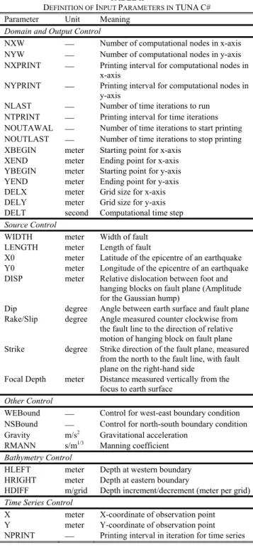
TABLEII

DEFINITION OF INPUT PARAMETERS IN TUNAC#

Parameter Unit Meaning

Domain and Output Control

NXW ⎯ Number of computational nodes in x-axis NYW ⎯ Number of computational nodes in y-axis NXPRINT ⎯ Printing interval for computational nodes in

x-axis

NYPRINT ⎯ Printing interval for computational nodes in y-axis

NLAST ⎯ Number of time iterations to run NTPRINT ⎯ Printing interval for time iterations NOUTAWAL ⎯ Number of time iterations to start printing NOUTLAST ⎯ Number of time iterations to stop printing XBEGIN meter Starting point for x-axis

XEND meter Ending point for x-axis YBEGIN meter Starting point for y-axis YEND meter Ending point for y-axis DELX meter Grid size for x-axis DELY meter Grid size for y-axis DELT second Computational time step Source Control

WIDTH meter Width of fault LENGTH meter Length of fault

X0 meter Latitude of the epicentre of an earthquake Y0 meter Longitude of the epicentre of an earthquake DISP meter Relative dislocation between foot and

hanging blocks on fault plane (Amplitude for the Gaussian hump)

Dip degree Angle between earth surface and fault plane Rake/Slip degree Angle measured counter clockwise from

the fault line to the direction of relative motion of hanging block on fault plane Strike degree Strike direction of the fault plane, measured

from the north to the fault line, with fault plane on the right-hand side

Focal Depth meter Distance measured vertically from the focus to earth surface

Other Control

WEBound ⎯ Control for west-east boundary condition NSBound ⎯ Control for north-south boundary condition Gravity m/s2 _{Gravitational acceleration}

RMANN s/m1/3 _{Manning coefficient} Bathymetry Control

HLEFT meter Depth at western boundary HRIGHT meter Depth at eastern boundary

HDIFF m/grid Depth increment/decrement (meter per grid) Time Series Control

X meter X-coordinate of observation point Y meter Y-coordinate of observation point NPRINT ⎯ Printing interval in iteration for time series

Fig. 9 refers to a tsunami simulation within a square computational domain of 10 km by 10 km (10000 m by 10000 m), with the south-west corner of the domain located at (XBEGIN, YBEGIN) = (0 m , 0 m) and the north-east corner located at (XEND, YEND) = (10000 m, 10000 m). This computational domain can easily be modified to suite a particular simulation scenario. The grid size is DELX = DELY = 100 m, while the time step DELT is 1 s. Both the

x-axis and y-axis are divided into 100 grids each, resulting in a total of NXW = NYW = 101 points in both x and y

directions respectively. The simulation is performed for a total of NLAST = 361 iterations, with output printed every NTPRINT = 40 iterations (or 40 s), beginning with iteration NOUTAWAL = 1. The results are to be printed for every NXPRINT = NYPRINT = 1 point in the x and y direction respectively. The initial tsunami source is given by the Gaussian formulation, describing a circle centred at the location (X0, Y0) = (5000 m, 5000 m), with a diameter of WIDTH = LENGTH = 2000 m. The domain has a constant depth of HLEFT = HRIGHT = 100 m (HDIFF = 0.0), resulting in a celerity of 31.32 m/s, with gravity of 9.81 m/s2. One (NPRINT = 1) time series of tsunami wave heights at the location (X, Y) = (5000 m, 5000 m) will be printed. However, more time series (NPRINT > 1) can also be printed by request. TUNA C# can accommodate up to several million nodes, which may take several hours to complete simulations.

The simulation results are demonstrated in Fig. 9, showing three snapshots, with the first snapshot at 40 s printed in Fig. 9 (left frame). The tsunami waves continue to propagate symmetrically outwards towards the square boundary and arrive at the boundary at the correct arrival time of 120 s (middle frame of Fig. 9), as correctly indicated by the celerity or travelling speed of 31.32 m/s. The waves subsequently pass through the open boundary with minimal reflection at 240 s (third frame of Fig. 9). It is noted that if the four square boundaries were to consist of solid walls that would reflect incoming waves, then the waves would reflect and would propagate backward from the solid boundary into the square to give rise to interaction of reflected waves inside the square, as shown in Fig. 10. These reflected waves and their interactions produce dangerous situations when tsunamis propagate into a semi-enclosed harbour. It is known that tsunami propagation speed or celerity depends on the depth of the sea through which they propagate. To demonstrate this dependence of speed of tsunami propagation on the ocean depth, we change the sea depth linearly from 100 m to 1000 m, the results of which are depicted in Fig. 11.

Fig. 9. Snapshots of tsunami propagation in a square domain with open boundaries.

Fig. 11 (top row) shows that the wave propagate with the uniform speed of 31.32 m/s, when the depth is a constant 100 m (HLEFT = HRIGHT = 100.0; HDIFF = 0.0). However, when the depth is increased linearly from HRIGHT = 100 m at the eastern boundary to HLEFT = 1000 m at the western boundary (HDIFF = − 9 m per grid), the waves propagate faster in the deeper western half, arriving at the western boundary earlier after 40 s but at the eastern boundary later at 80 s (Fig. 11, middle row). On the other hand when the depth is increased linearly from HLEFT = 100 m at the western (shallower) boundary to HRIGHT = 1000 m at the eastern (deeper) boundary (HDIFF = + 9 m per grid), the propagation speed pattern is reversed. The waves arrive at the deeper eastern boundary earlier after 40 s but arrive at the shallower western boundary later at 80 s (Fig. 11, bottom row).

Fig. 11. Snapshots of tsunami propagation in a square domain with constant and linear depth.

V. CONCLUSION

This paper presents a brief review of tsunami simulations performed by TUNA for the Andaman Sea and the South China Sea to highlight potential tsunami hazards to the affected coastal regions. To help develop human capacity to conduct tsunami risk simulation, a series of workshops had been conducted in the region. A summary of these workshops and the associated model manual is presented to facilitate tsunami simulation training.

REFERENCES

[1] L. Sternberg, S.Y. Teh, S. Ewe, F.R. Miralles-Wilhelm and D. DeAngelis, “Competition between hardwood hammocks and mangroves”, Ecosystems 10(4), 2007, 648-660.

[2] S.Y. Teh, D. DeAngelis, L. Sternberg, F.R. Miralles-Wilhelm, T.J. Smith and H.L. Koh, “A simulation model for projecting changes in salinity concentrations and species dominance in the coastal margin habitats of the Everglades”, Ecological Modelling 213(2), 2008, 245-256.

[3] H.L. Koh, S.Y. Teh, P.L.-F. Liu, A.M.I. Izani and H.L. Lee, “Simulation of Andaman 2004 tsunami for assessing impact on Malaysia”, Journal of Asian Earth Sciences 36(1), 2009, 74-83. [4] H.L. Koh, S.Y. Teh, A.M.I. Izani, H.L. Lee and L.M. Kew,

“Simulation of future Andaman tsunami into Straits of Malacca by TUNA”, Journal of Earthquakes and Tsunamis 3(2), 2009, 89-100. [5] H.L. Koh, S.Y. Teh, H.L. Lee and A.M.I. Izani, “Modeling Andaman

tsunami runup through Penang mangrove forest”, Chapter 1: Monitoring and Modeling of Water Environment, In: Southeast Asian Water Environment 3, Satoshi Takizawa, Futoshi Kurisu and Hiroyasu Satoh (Eds.), IWA Publishing, London, UK, 2009, pp. 51-56.

[6] S.Y. Teh and H.L. Koh, “Simulation of tsunami generated by the Manila trench”, Proceedings of the 2010 3rd International Conference on Environmental and Computer Science (ICECS 2010), 18-19 October 2010, Kunming, China, International Association of Computer Science & Information Technology (IACSIT), IEEE Computer Society, 2010, pp. 20-24.

[7] H.L. Koh, D.L. DeAngelis and S.Y. Teh, “Mangrove wetland ecosystem modeling in the Everglades”, In: Mangroves: Ecology, Biology and Taxonomy. Nova Science Publishers, Inc., Hauppauge, New York (in press).

[8] H.L. Koh, S.Y. Teh, P.L.-F.Liu and M.R. Che Abas, “Tsunami simulation research and mitigation programs in Malaysia post 2004 Andaman tsunami”, In: Tsunamis: Causes, Characteristics and Warnings, and Protection, Neil Veitch and Gordon Jaffray (Eds.). Nova Science Publishers, Inc., Hauppauge, New York, 2010, pp. 29-56.

[9] H.L. Koh, S.Y. Teh, T.A. Majid and H. Abdul Aziz, “Grid computing for disaster mitigation”, In: Data Driven e-Science: Use Cases and Successful Applications of Distributed Computing Infrastructures (ISGC 2010), Simon C. Lin and Eric Yen (Eds), Springer, New York (in press).

[10] IOC, “Numerical method of tsunami simulation with the leap frog scheme, 1, shallow water theory and its difference scheme”. In Manuals and Guides of the IOC, Intergovernmental Oceanogr. Comm., UNESCO, Paris, 1997, pp. 12-19.

[11] H. Hérbert, F. Schindelé, Y. Altinok, B. Alpar and C. Gazioglu, “Tsunami hazard in the Marmara Sea (Turkey): a numerical approach to discuss active faulting and impact on the Istanbul coastal areas”, Marine Geology 215, 2005, 23-43.

[12] H.L. Koh, S.Y. Teh and A.M.I. Izani, “Tsunami mitigation management”, Special Feature: Natural Disaster Management Technologies, The United Nations Asian and Pacific Centre for Transfer of Technology (UN-APCTT) Nov-Dec 2007, Asia Pacific Tech Monitor 24(6), 2007, 47-54.

[13] S.B. Yoon, “Propagation of distant tsunamis over slowly varying topography”, J Geophys Res 107 (C10), American Geophysical Union, 2002, 4.1-4.11.

[14] S.B. Yoon and P.L.F. Liu, “Numerical simulation of a distant small-scale tsunami”, In: Recent Advances in Marine Science and Technology: PACON92, Pac. Congr. On Mar. Sci. And Technol., Kona, Hawaii, N. Saxena (Ed.), 1992, pp. 67-78.

[15] S.Y. Teh, H.L. Koh, P.L.-F Liu., A.M.I. Izani and H.L. Lee, “Analytical and numerical simulation of tsunami mitigation by mangroves in Penang, Malaysia”, Journal of Asian Earth Sciences 36(1), 2009, 38-46.

[16] F. Imamura, N. Shuto and C. Goto, “Numerical simulation of the transoceanic propagation of tsunamis”, Proceeding of the Sixth Congress of the Asian and Pacific Regional Division, Int. Assoc. Hydraul. Res., Kyoto, Japan, 1988, pp. 265-272.

[17] V.V. Titov, “Numerical modeling of long wave runup”, Ph.D. Thesis, University of Southern California, Los Angeles, CA, 1997, 150 p. [18] S.Y. Teh, “Modeling Evolution of Tsunami and Its Impact on Coastal

Vegetation”, PhD Thesis, Universiti Sains Malaysia, Penang, Malaysia, 2008, 197 p.

[19] P.L.-F. Liu, S.B. Woo and Y.S. Cho, “Computer programs for tsunami propagation and inundation”, Cornell University, Sponsored by National Science Foundation, 1998, 104 p.

[20] Y. Okada, “Surface deformation due to shear and tensile faults in a half-space”, Bull. Seismol. Soc. Am. 75(4), 1985,1135-1154. [21] S.T. Grilli, M. Ioualalen, J. Asavanant, F. Shi, J. Kirby, and P. Watts,

“Source constraints and model simulation of the December 26, 2004 Indian Ocean Tsunami”, J. Waterw. Port Coast. Ocean Eng. 133 (6), 2007, 414–428.

[22] P.L.-F. Liu, X. Wang and A.J. Salisbury, “Tsunami hazard and early warning system in South China Sea”, Journal of Asian Earth Sciences 36(1), 2009, 2-12.

[23] M.J.R. Gee, H.S. Uy, J. Warren, C.K. Morley and J.J. Lambiase, “The Brunei slide: a giant submarine landslide on the North West Borneo Margin revealed by 3D seismic data”, Marine Geology 246(1), 2007, 9-23.