Cirrus clouds in a global climate model with a statistical cirrus cloud scheme

(1)

ACPD

9, 16607–16682, 2009

Cirrus clouds in a global climate model

M. Wang and J. E. Penner

Title Page

Abstract Introduction

Conclusions References

Tables Figures

◭ ◮

Back Close

Full Screen / Esc

Printer-friendly Version

Interactive Discussion

Atmos. Chem. Phys. Discuss., 9, 16607–16682, 2009 www.atmos-chem-phys-discuss.net/9/16607/2009/ © Author(s) 2009. This work is distributed under the Creative Commons Attribution 3.0 License.

Atmospheric Chemistry and Physics Discussions

This discussion paper is/has been under review for the journalAtmospheric Chemistry and Physics (ACP). Please refer to the corresponding final paper inACPif available.

Cirrus clouds in a global climate model

with a statistical cirrus cloud scheme

M. Wang1,*and J. E. Penner1

1

Department of Atmospheric, Oceanic, and Space Sciences, University of Michigan, USA

*

now at: Pacific Northwest National Laboratory, Richland, Washington, USA

Received: 18 June 2009 – Accepted: 30 July 2009 – Published: 7 August 2009

Correspondence to: M. Wang (minghuai.wang@pnl.gov)

(2)

ACPD

9, 16607–16682, 2009

Title Page

Tables Figures

◭ ◮

Back Close

Full Screen / Esc

Interactive Discussion Abstract

A statistical cirrus cloud scheme that accounts for mesoscale temperature perturba-tions is implemented into a coupled aerosol and atmospheric circulation model to bet-ter represent both cloud fraction and subgrid-scale supersaturation in global climate models. This new scheme is able to better simulate the observed probability

distri-5

bution of relative humidity than the scheme that was implemented in an older version of the model. Heterogeneous ice nuclei (IN) are shown to affect not only high level cirrus clouds through their e_ffect on ice crystal number concentration but also low level liquid clouds through the moistening effect of settling and evaporating ice crystals. As a result, the change in the net cloud forcing is not very sensitive to the change in ice

10

crystal concentrations associated with heterogeneous IN because changes in high cir-rus clouds and low level liquid clouds tend to cancel. Nevertheless, the change in the net radiative flux at the top of the atmosphere due to changes in IN is still large be-cause of changes in the greenhouse e_ffect of water vapor caused by the changes in ice crystal number concentrations. Changes in the magnitude of the assumed mesoscale

15

temperature perturbations by 25% alter the ice crystal number concentrations and ra-diative fluxes by an amount that is similar to that from a factor of 10 change in the heterogeneous IN number concentrations.

1 Introduction

Cirrus clouds cover about 30% of the Earth’s area (Wang et al., 1996; Rossow and

20

Schiffer, 1999; Wylie and Menzel, 1999) and are important in maintaining the global ra-diation balance (Ramanathan and Collins, 1991). They can form through either homo-geneous freezing or heterohomo-geneous freezing. Homohomo-geneous freezing occurs through the freezing of liquid solutions such as sulfate droplets (Koop et al., 2000), and this usually occurs at low temperature and high relative humidity over ice (RHi). In

con-25

(3)

ACPD

9, 16607–16682, 2009

Title Page

Tables Figures

◭ ◮

Back Close

Full Screen / Esc

1997) or surfactant layers (Zobrist et al., 2007) that lower the energy barrier for the formation of an ice germ, and therefore requires lower supersaturation and can occur at higher temperatures. Aerosol particles that contribute such surfaces and undergo heterogeneous freezing are termed ice nuclei (IN). Mineral dust, carbonaceous, and metallic particles appear to be common heterogeneous IN (Chen et al., 1998; DeMott

5

et al., 2003; Cziczo et al., 2004, 2009).

Homogeneous freezing is believed to be the primary mechanism for cirrus cloud for-mation in cold environments with high updraft velocities (e.g., Heymsfield and Sabin, 1989; Cantrell and Heymsfield, 2005), but the presence of heterogeneous IN can de-crease the occurrence of homogeneous freezing because of the consumption of water

10

vapor that prevents the formation of the high RHi needed (e.g., Demott et al., 1997; Liu and Penner, 2005). This preventive e_ffect may significantly change cirrus cloud properties and humidity in the upper troposphere. Heterogeneous freezing from a few IN may result in lower ice crystal number concentrations and larger ice crystal par-ticles than those from homogeneous freezing, since homogeneous freezing usually

15

generates high concentrations of ice crystals because of the abundance of liquid haze particles. Jensen et al. (2008) suggested that it is likely that the observed presence of rather large ice crystals near the tropical tropopause in very low concentrations results from ice nucleation on effective heterogeneous IN. Heterogeneous freezing may also change the frequency of occurrence of cirrus clouds because of the lower RHi and

20

thus its more frequent occurrence (Jensen and Toon, 1997). Haag and K ¨archer (2004) used a Lagrangian microphysical aerosol-cloud model to show that the frequency of occurrence of thin cirrus clouds can be changed significantly as a result of the pres-ence of a small number of IN at midlatitudes. Heterogeneous freezing may also change ice water content by changing ice crystal settling velocities (e.g., Haag and K ¨archer,

25

(4)

ACPD

9, 16607–16682, 2009

Title Page

Tables Figures

◭ ◮

Back Close

Full Screen / Esc

(INCA) field experiments could be explained by heterogeneous freezing from the in-creased number of aerosol particles that act as IN in the NH.

The calculation of the effect of heterogeneous IN on cirrus cloud properties is compli-cated by the fact that small scale dynamical processes play an important role in ice nu-cleation in the upper troposphere (e.g., Heymsfield, 1977; Str ¨om et al., 1997; K ¨archer

5

and Str ¨om, 2003; Haag and K ¨archer, 2004; Jensen and Pfister, 2004; Hoyle et al., 2005). Small scale dynamical processes control the cooling rates within parcels that form cirrus clouds, which, together with the ambient temperature determines whether heterogenous or homogeneous freezing dominates the ice nucleation process. Heyms-field (1977) found that the ice crystal concentration and ice water content in cirrus

10

clouds are strong functions of the vertical velocity based on airborne measurements in the United States. Str ¨om et al. (1997) demonstrated the potential impact of atmo-spheric waves on the physical properties of young cirrus clouds from airborne measure-ments over Southern Germany. Immler et al. (2008) found a clear correlation between temperature anomalies induced by equatorial Kelvin waves and the occurrence of thin

15

cirrus at the tropical tropopause. The strong role of small scale dynamical processes on ice nucleation and cirrus cloud microphysical properties make it di_fficult to separate the e_ffects of aerosol changes and dynamical changes on cirrus microphysical proper-ties (K ¨archer and Str ¨om, 2003). It has been suggested that cirrus formation is at least as sensitive to changes in dynamical forcing patterns as to changes in the aerosol size

20

and number (K ¨archer and Str ¨om, 2003).

Global models have been used recently to study the effect of homogeneous and heterogeneous freezing on cirrus cloud properties (Lohmann and K ¨archer, 2002; Hen-dricks et al., 2005; Liu et al., 2009). In these studies, the individual GCMs were up-dated to allow supersaturation with respect to ice, but cloud fraction was still diagnosed

25

(5)

ACPD

9, 16607–16682, 2009

Title Page

Tables Figures

◭ ◮

Back Close

Full Screen / Esc

100%. Partial cloud cover is only diagnosed when subsaturation subsequently occurs. The representation of subgrid-scale fluctuations of temperature, humidity, and cooling rates that are believed to control the cirrus cloud microphysical formation process and the related microphysical cirrus cloud properties, are highly simplified in these studies. The simulated effects of subgrid-scale fluctuations are only represented in the

calcu-5

lation of ice crystal number concentrations while the cloud fraction changes depend only on the grid-mean relative humidity. The simplifications in these models limit their capability to study aerosol indirect effects on cirrus clouds.

To address the inconsistency between the diagnosis of cloud fraction and the pre-diction of ice supersaturation, Tompkins et al. (2007) used a prognostic cloud

frac-10

tion that is consistent with their predicted ice supersaturation in the European Centre for Medium-Range Weather Forecasts (ECMWF) Integrated Forecast System. This scheme uses clear sky relative humidity to determine when ice freezing occurs and how much cloud fraction increases. However, this scheme has highly simplified ice microphysics (no ice crystal number is predicted). Moreover, this study assumed vapor

15

saturation in cloudy air. In observations, both ice supersaturation and subsaturation conditions can occur in cloudy air (Str ¨om et al., 2003). For example, significant su-persaturation can occur when ice crystal number concentration is low (Kr ¨amer et al., 2009), and subsaturation can occur when ice crystal particles are large (Hall and Prup-pacher, 1976).

20

K ¨archer and Burkhardt (2008, hereafter KB08) presented a statistical cloud scheme for non-convective cirrus formed by homogeneous freezing of supercooled aerosols, which treats cloud growth and decay based on a subgrid-scale distribution of tempera-ture and total water. The scheme is based on separate probability distribution functions for total water in the clear-sky and cloudy sky portions of each grid. These distributions

25

(6)

ACPD

9, 16607–16682, 2009

Title Page

Tables Figures

◭ ◮

Back Close

Full Screen / Esc

In this study, the cirrus cloud scheme in KB08 is implemented in the updated ver-sion of NCAR CAM3 (Liu et al., 2007a, hereafter LIU07) which has been coupled with the LLNL/UMich IMPACT aerosol model (Wang et al., 2009), in order to replace the cirrus cloud treatment in LIU07. We have extended the KB08 scheme to include both homogeneous freezing and heterogeneous freezing. Anvil clouds from convective

de-5

trainment are also included and compete for water vapor with large scale cirrus clouds in the clear sky portion of each grid. The coupled model and the implementation of KB08 are presented in Sect. 2, and model results in the case of homogeneous freez-ing only are shown in Sect. 3. The e_ffects of heterogeneous IN and changes to the assumed probability density function of the subgrid scale temperature perturbations

10

are examined in Sect. 4. Finally, Sect. 5 contains a discussion and conclusions.

2 Model description and set-up of simulations

The fully coupled IMPACT aerosol model and NCAR CAM3 model (Wang et al., 2009) are used in this study. The two model components of the coupled system are concur-rently run in MPMD (Multiple Processors Multiple Data) mode to exchange aerosol

15

fields and meteorological fields at each advection time step of the IMPACT model (Wang et al., 2009).

2.1 The IMPACT global aerosol model

In this study, the mass-only version of the Lawrence Livermore National Laboratory (LLNL)/University of Michigan IMPACT model was used, which predicts aerosol mass,

20

but not number (Liu and Penner, 2002). We choose the mass-only version of the IMPACT model instead of the complete aerosol microphysics version used in Wang et al. (2009) because the mass-only version of the model is computationally fast which allowed us to run more sensitivity studies.

The mass-only version of IMPACT includes prognostic variables for sulfur and

(7)

ACPD

9, 16607–16682, 2009

Title Page

Tables Figures

◭ ◮

Back Close

Full Screen / Esc

lated species: dimethylsulfide (DMS), sulfur dioxide (SO₂), sulfate aerosol (SO2₄−), and hydrogen peroxide (H₂O₂); aerosols from biomass burning black carbon (BC) and organic matter (OM), fossil fuel BC and OM, natural OM, aircraft BC (soot), min-eral dust, and sea salt are also included. Sulfate aerosol is divided into three size bins with radii varying from 0.01–0.05µm, 0.05–0.63µm and 0.63–1.26µm, while

5

mineral dust and sea salt are predicted in four bins with radii varying from 0.05– 0.63µm, 0.63–1.26µm, 1.26–2.5µm, and 2.5–10µm. Carbonaceous aerosol (OM and BC) is currently represented by a single submicron size bin. Emissions of pri-mary particles and precursor gases, gas-phase oxidation of precursor gases, aqueous-phase chemistry, rain-out and washout, gravitational settling, and dry deposition are

10

treated. The mass-only version of the IMPACT aerosol model driven by meteorolog-ical fields from the NASA Data Assimilation O_ffice (DAO) participated in the AERO-COM (http://nansen.ipsl.jussieu.fr/AEROAERO-COM/) phase A and B evaluations (Kinne et al., 2006; Textor et al., 2006; Schulz et al., 2006), where it has been extensively com-pared with in situ and remotely sensed data for different aerosol properties.

15

Emissions of aerosol species and their precursors are described in detail in Wang et al. (2009). Anthropogenic sulfur emissions were from Smith et al. (2001, 2004), for the year 2000 (61.3 Tg S per year). Anthropogenic emissions of fossil fuel and biomass burning carbonaceous aerosols were from Ito and Penner (2005) for the year 2000, but adjusted as discussed in Wang et al. (2009). The fossil fuel BC and OM emissions were

20

5.8 Tg BC and 15.8 Tg OM per year, and the biomass burning BC and OM emissions were 4.7 Tg BC and 47.4 Tg OM per year. Emissions of BC from aircraft were 0.0034 Tg per year based on the fuel use model of Lee et al. (2005) with emission factors from AERO2K (Eyers et al., 2004). Natural emissions included volcanic SO₂ (4.79 Tg S per year from Andres and Kasgnoc, 1998), marine dimethyl sulfide (DMS) (26.1 Tg S

25

(8)

ACPD

9, 16607–16682, 2009

Title Page

Tables Figures

◭ ◮

Back Close

Full Screen / Esc

model using the method defined in Gong et al. (1997).

Prescribed size distributions from observations were used to calculate the number concentrations of sulfate, dust and soot particles that are used in the ice particle nucle-ation parameteriznucle-ation described in Sect. 2.2. Sulfate particles were assumed to have a lognormal size distribution with a mode radius of 0.02µm and a geometric standard

5

deviation of 2.3 (Jensen et al., 1994). For soot particles emitted from the Earth’s sur-face (i.e., biomass burning and fossil fuel combustion), we assumed a size distribution with a mode radius of 0.07µm and a geometric standard deviation of 1.5 (Pueschel et al., 1992). Aircraft soot has a much smaller size with a mode radius of 0.023µm and a geometric standard deviation of 1.5 (Petzold and Schr ¨oder, 1998). The size distribution

10

of dust particles (Table B1) is taken from De Reus et al. (2000).

2.2 NCAR CAM3

The NCAR Community Atmospheric Model (CAM3) is part of the Community Climate System Model 3 (CCSM3; Collins et al., 2006a, b). The model predicts both cloud liquid water and cloud ice water (Boville et al., 2006). Cloud condensate detrained from deep

15

and shallow convection is added into stratiform clouds. The gravitational settling as well as large-scale transport of cloud condensate is separately treated for cloud liquid and ice (Boville et al., 2006). However, in the standard CAM3, the partitioning between cloud liquid and cloud ice depends only on temperature (T), and both the cloud droplet number and ice crystal number used in the cloud microphysics scheme are prescribed.

20

Therefore, CAM3 is not able to represent a variety of processes (e.g., the Bergeron-Findeisen process, ice nucleation, droplet nucleation) that are important to the study of aerosol-cloud interactions.

The standard CAM3 version was updated in LIU07, by introducing a two-moment cloud microphysics scheme for ice cloud, in which cloud ice number concentrations

25

(9)

ACPD

9, 16607–16682, 2009

Title Page

Tables Figures

◭ ◮

Back Close

Full Screen / Esc

standard version of CAM3. This is accomplished by explicitly treating the liquid mass conversion to ice due to the depositonal growth of cloud ice at the expense of liquid water (the Bergeron-Findeisen process) using the scheme of Rotstayn et al. (2000). This replaces the simple temperature-dependent liquid/ice partitioning in the standard CAM3. The cloud condensation and evaporation (C-E) scheme of Zhang et al. (2003)

5

in the standard CAM3 is used only for liquid water in warm (T >0◦C) and mixed-phase (₋35◦C<T <0◦C) clouds, which removes any supersaturation above that of liquid wa-ter. Vapor deposition and sublimation of cloud ice is treated based on Rotstayn et al. (2000). With these modifications, supersaturation over ice is allowed in the upper troposphere. The coupled model with the ice cloud treatment in LIU07 has been used

10

to study the e_ffects of aerosols on cirrus clouds (Liu et al., 2009).

In LIU07, although supersaturation with respect to ice is allowed, cirrus cloud fraction is still diagnosed based on the grid-mean relative humidity, as described in Rasch and Kristj ´ansson (1998). This leads to an inconsistency between increases in cirrus cloud fraction and new cloud formation by ice nucleation. For example, new cloud formation

15

by ice nucleation requires an RHi of about 125% (heterogeneous freezing) or 150% (homogeneous freezing), but the cloud fraction in LIU07 begins to increase at an RHi

of 90%. This causes a large increase in the cirrus cloud fraction in LIU07 (56.8%) compared to the standard CAM3 (32.2%). Moreover, the grid-mean saturation ratio was used to initiate the parameterization of homogeneous freezing or heterogeneous

20

freezing in LIU07, although mesoscale motions such as gravity waves were accounted for using a sub-grid variation of the updraft. Here, in order to treat cirrus cloud formation in a consistent manner in the upper troposphere, the statistical cirrus cloud scheme presented in KB08 was implemented in CAM3, replacing the cirrus cloud treatment of LIU07. This new scheme has subgrid-scale features for clear sky temperature and

25

(10)

ACPD

9, 16607–16682, 2009

Title Page

Tables Figures

◭ ◮

Back Close

Full Screen / Esc

In the new cirrus cloud scheme, the specific humidity in both the clear sky areas (q_ve) and cloudy areas (qvc) within a grid is predicted in the model. The specific humidity in

the clear sky area is used to determine whether ice nucleation occurs and how much cloud fraction will increase as a result of any freezing, while the specific humidity in the cloudy part of the grid box is used to determine whether vapor deposition or evaporation

5

occurs and is used to determine how much cloud fraction decreases in the case of evaporation. The grid mean specific humidity (q_v) is calculated as aq_vc+(1₋a)q_ve, whereais the cloud fraction.

Cloud growth is determined by the mean specific humidity in the clear part of a grid box using an assumed subgrid variation in the temperature profile. As shown in

previ-10

ous studies (KB08; Hoyle et al., 2005; K ärcher and Str öm, 2003; Haag and K ärcher, 2004; Jensen and Pfister, 2004), the use of large scale temperature fluctuations alone is not sufficient for ice nucleation in cirrus clouds, and mesoscale temperature fluctua-tions from small scale mofluctua-tions such as gravity waves are critical to cirrus cloud genera-tion and to the determinagenera-tion of cirrus cloud properties. These mesoscale temperature

15

fluctuations cover horizontal length-scales 1–100 km (Str ¨om et al., 1997; Bacmeister et al., 1999) and arise from a variety of sources. These sources include intense gravity waves released by mesoscale convective systems, high amplitude lee waves induced by high mountain ridges, or high amplitude lee waves induced in the area of jet streams and storm tracks (KB08). Even away from main source areas, there appears to be

20

a persistent background of mesoscale temperature fluctuations driven by mesoscale gravity waves (Gary, 2006, 2008).

In the new cirrus cloud scheme, a probability density function (PDF) of temperature is used to represent mesoscale temperature perturbations in the clear sky portion of a grid. The PDF of temperature (dP_T/dT) is assumed to be a constrained normal

dis-25

tribution with a mean temperature (T0) that is predicted by the GCM, and a standard

(11)

ACPD

9, 16607–16682, 2009

Title Page

Tables Figures

◭ ◮

Back Close

Full Screen / Esc

PDF of the temperature distribution is then transformed into a PDF of the saturation ratio (S) (dP_S/dS) (Eq. A2) using the saturation vapor pressure over pure hexagonal ice (Murphy and Koop, 2005) and the mean specific humidity in the clear sky part of the grid (q_ve). By comparing the PDF of S with the freezing threshold saturation ratio (Scr), we can determine the portion of the distribution that is located aboveScr as:

5

f(S > S_cr)=

ZS₃₊

Scr

d PS

d S d S, (1)

whereS₃₊is the upper bound of the saturation ratio over whichdP_S/dSis defined (see Eq. A2). Ice crystals form whendPs/dS extends above the freezing threshold. After taking account of the clear sky fraction (1₋a), we have cloud fraction increases from ice nucleation defined as

10

∆a=(1₋a)f(S > Scr). (2)

The increase in the grid-mean ice crystal number concentration (ni) from ice

nucle-ation is then

∆ni =Ni∆a, (3)

whereN_i is the in-cloud ice crystal number concentration from homogeneous freezing

15

and/or heterogeneous freezing. When both homogeneous freezing and heterogeneous freezing is allowed, ifS is greater than the critical saturation ratio for heterogeneous freezing, but lower than that required for homogeneous freezing, thenN_i is determined by the number of heterogeneous nuclei. IfS is greater than the critical saturation ratio for homogeneous freezing, thenNi is set to the sum of the heterogeneous nuclei plus

20

the homogeneous nuclei, as discussed in detail later (Eqs. 6–9).

To calculateN_i, vertical velocities or cooling rates are needed, and are parameter-ized based on the probability distribution forδT. The mean cooling rate̟, induced by mesoscale temperature fluctuations, is approximated by

̟[K h−1]₌8.2δT[K], (4)

(12)

ACPD

9, 16607–16682, 2009

Title Page

Tables Figures

◭ ◮

Back Close

Full Screen / Esc

as in Hoyle et al. (2005); then the mean vertical velocity ( ¯w) is deduced by assuming that the cooling takes place in a parcel lifting adiabatically. This cooling rate or vertical velocity is then used to calculate the ice crystal number concentration. For homoge-neous freezing, the resulting ice crystal number densityN_i _homois approximated as

Ni homo≈2n( ¯w), (5)

5

wheren( ¯w) is the ice crystal number concentration from the homogeneous freezing parameterization for the vertical velocity, ¯w. This formula is based on the integration of the PDF of vertical velocity or cooling rate, and takes account of the following two factors: (a) most of the small cooling rates do not contribute to freezing on average, and (b) high ice crystal concentrations resulting from high cooling rates are more effective

10

at suppressing subsequent supersaturation (KB08).

KB08 demonstrated that aδT of 1 K reproduces the observed distribution of satu-ration ratios at temperatures near 225 K, as measured in the middle latitudes of both hemispheres from INCA field data (K ¨archer and Str ¨om, 2003; KB08). AδT of 1 K is also close to the average mesoscale temperature amplitudes associated with mean

15

mesoscale altitude displacements of air parcels of_∼100 m as inferred from analysis of Microwave Temperature Profiler data by Gary (2006, 2008), who analyzed data from more than 4000 aircraft flight hours taken in the altitude range 7–22 km and with a va-riety of underlying topography, spanning the latitude range 70◦S to 80◦N. Gary (2006) also showed that the mesoscale temperature amplitudes increase with altitude, which

20

is consistent with the gravity wave theory (Fritts and Alexander, 2003).

By using Eq. (4), a δT of 1 K gives a cooling rate of 8.2 K/hour and a vertical ve-locity of 23 cm/s, which is close to the mean vertical veve-locity of 26 cm/s measured in the updraught regions in the INCA campaign (K ¨archer and Str ¨om, 2003). However, it is not known whether the mean updraft velocity of 23 cm/s is representative at other

25

(13)

ACPD

9, 16607–16682, 2009

Title Page

Tables Figures

◭ ◮

Back Close

Full Screen / Esc

use of this velocity causes ice crystal number concentrations that are too high at low temperatures. For example, a vertical velocity of_∼20 cm/s would predict an ice crystal number concentration of order 10 cm−3at a temperature of 193 K from homogeneous freezing for a sulfate particle number concentration of 50 cm−3, but such high ice crystal number concentrations at these temperatures are not supported by field observations.

5

Kr ¨amer et al. (2009) examined aircraft in-situ observations of ice crystal number con-centration from 28 flights in tropical, midlatitude, and Arctic field experiments in the temperature range of 183–250 K and showed that ice crystal number concentrations decreased with decreasing temperature. This decrease in ice crystal number concen-trations cannot be reproduced if a constant vertical velocity perturbation is assumed

10

when homogeneous freezing dominates at these levels. A vertical velocity as low as 1 cm/s is able to explain the observed ice crystal number concentrations at very low temperatures, however. Although a decrease in ice crystal number concentrations might also be achieved by changing the number of heterogeneous IN with tempera-ture, we note that vertical velocities of around 1 cm/s were used in Khvorostyanov et

15

al. (2006) and Jensen et al. (2008), and that these were able to reproduce the ob-served ice crystal number concentration for thin tropopause cirrus from homogeneous freezing during the 2004 CRYSTAL-FACE and 2006 CRAVE campaigns, respectively. Thus, we assumed a linear decrease in the vertical velocity fluctuation with decreasing temperature from 23 cm/s at 238 K to 1.2 cm/s at 193 K and a constant velocity outside

20

these extremes. This results in a mesoscale temperature perturbation of 1 K at 238 K and 0.05 K at 193 K (or below) using Eq. (4).

In KB08, homogeneous freezing is the only freezing mode for cirrus clouds. In this study, an additional scenario that allows competition between homogeneous and het-erogeneous freezing is included. When homogeneous freezing is the only freezing

25

mode, ice crystal number concentration from ice freezing (Ni homo) and the threshold

freezing saturation ratio (Scr homo) are parameterized based on Liu and Penner (2005),

(14)

concentra-ACPD

9, 16607–16682, 2009

Title Page

Tables Figures

◭ ◮

Back Close

Full Screen / Esc

tion. In the scenario where competition between homogeneous freezing and hetero-geneous freezing is allowed,Scr homoand the adjustedNi homo(Eq. 5) are still used to

determine the increase in cloud fraction and ice crystal number concentration due to homogeneous freezing. But when the heterogeneous IN number concentration (N_{i n}) exceeds the threshold IN number concentration (Ni n cr) derived in Gierens (2003),

5

heterogeneous freezing is allowed. The heterogeneous freezing threshold saturation ratio (S_cr _hete) and ice crystal number concentration from heterogeneous ice freezing (Ni hete) are parameterized based on Liu and Penner (2005) and then used to

calcu-late the total cloud fraction increase and the change in ice crystal number concentration from heterogeneous freezing. The ice number from heterogeneous freezing is not

mul-10

tiplied by a factor of 2, since the factor of 2 applied for homogeneous freezing is primar-ily used to account for the nonlinear dependence of ice crystal number concentrations on vertical velocity. The number of ice crystals formed from heterogeneous freezing is not as sensitive to changes in vertical velocity as those from homogeneous freez-ing. For example, at temperature 225 K, when vertical velocities increase from 10 cm/s

15

to 50 cm/s, heterogeneous ice crystal number concentrations that are parameterized based on Liu and Penner (2005) change very little for a soot number concentration less than 0.1 cm−3, while homogeneous ice crystal number concentrations increase from 0.20 cm−3 to 2.50 cm−3 for a sulfate particle number concentration of 50 cm−3. So, the cloud fraction increase and ice crystal number concentration increase in the

20

scenario with both homogeneous and heterogeneous freezing was defined as:

∆a=(1₋a)f(S > S_cr _homo), (6)

∆n_i =N_i _homo∆a, whenN_{i n}< N_{i n cr} (7)

and

∆a=(1₋a)f(S > S_cr _hete), (8)

25

(15)

ACPD

9, 16607–16682, 2009

Title Page

Tables Figures

◭ ◮

Back Close

Full Screen / Esc

whereN_i _homo (increased by a factor of 2, see Eq. 5) andN_i _hete are evaluated at the average updraft velocity ¯w.

In the treatment with both homogeneous freezing and heterogeneous freezing, het-erogeneous freezing is only allowed to occur when the concentration of heteroge-neous IN exceeds the critical heterogeheteroge-neous IN concentration. However, in the real

5

atmosphere, when the saturation ratio exceeds the freezing threshold saturation ratio, heterogeneous freezing occurs once heterogeneous IN are present, regardless of the concentration of the heterogeneous IN. This implies that Eqs. (8) and (9) should always be applied when the saturation ratio is larger than the freezing threshold saturation ra-tio. But given the large time step used in the NCAR CAM3 (30 min), the application of

10

Eqs. (8) and (9) without a limitation set by the number of heterogeneous IN concentra-tions would significantly decrease supersaturation levels in the model and result in very few homogeneous freezing events even when the concentration of heterogeneous IN is very low (<1/L). So in our treatment (and that by Liu et al., 2009), the competition between homogeneous freezing and heterogeneous freezing is partially parameterized

15

by using the critical heterogeneous IN concentration. When the heterogeneous IN con-centration is lower than the critical heterogeneous IN concon-centrations, heterogeneous freezing will not occur and the heterogeneous IN concentration is assumed to have no effect on homogeneous freezing.

Parcel model results may be used to quantify how accurate the treatment given in

20

Eqs. (6–9) is. Liu and Penner (2005) showed that when the heterogeneous IN con-centration is larger than N_{i n cr}, the ice crystal number concentration is determined by heterogeneous freezing. There is a transition region for heterogeneous IN num-ber concentrations fromNi n cr/10 toNi n cr, in which ice crystal number concentrations

gradually decrease from those determined by homogeneous freezing to those

deter-25

mined by heterogeneous freezing. When heterogeneous IN concentration are lower

than Ni n cr/10, ice crystal number concentrations are determined by homogeneous

(16)

con-ACPD

9, 16607–16682, 2009

Title Page

Tables Figures

◭ ◮

Back Close

Full Screen / Esc

centrations (>N_{i n cr}). However, when the concentration of heterogeneous IN is in the transition region (from Ni n cr/10 to Ni n cr), heterogeneous freezing is not allowed in

our treatment, and ice crystal number concentration is determined by homogeneous freezing. Ice crystal number concentrations may then be overestimated, and biased toward the ice crystal number concentration given by homogeneous freezing.

5

Here we use the critical heterogeneous IN concentration derived by Gierens (2003) to determine whether heterogeneous freezing will occur. In this formulation, the thresh-old IN number concentration (Ni n cr) is a function ofScr homo, Scr hete, vertical velocity,

temperature, and pressure (Gierens, 2003). Liu and Penner (2005) obtained a similar formula by empirically fittingN_{i n cr} as a function of vertical velocity from their parcel

10

model simulations. As shown in Liu and Penner (2005), the two formulas give

sim-ilar N_{i n cr} for vertical velocities larger than 20 cm/s. It was further shown by Liu et

al. (2009) that simulated changes in cirrus cloud properties and cloud forcing due to anthropogenic aerosols are very similar from these two formulas, when a subgrid scale PDF of vertical velocities with a mean of 0 and a standard deviation of 25 cm/s is

15

used. However, at low vertical velocities (less than 5 cm/s),N_{i n cr} from Liu and Pen-ner (2005) is much smaller than that from Gierens (2003). For example, at 193 K, with a vertical velocity of 1.2 cm/s,Ni n cr is 6.13×10−6cm−3in Liu and Penner (2005) and

is 6.12_×10−3 in Gierens (2003). Heterogeneous freezing occurs exclusively at very low vertical velocities when the formula in Liu and Penner (2005) is used. Therefore,

20

the formula of Gierens (2003) is used rather that that of Liu and Penner (2005) mainly because vertical velocities are restricted to low values at low temperatures in this study. The use of the Liu and Penner (2005) values forNi n cr would lead to concentrations

of ice crystal number concentrations that are lower than the observations of Kr ¨amer et al. (2009) when heterogeneous IN number concentrations are low. The source of

25

heterogeneous IN used in the model is discussed in Sect. 2.3.

(17)

ACPD

9, 16607–16682, 2009

Title Page

Tables Figures

◭ ◮

Back Close

Full Screen / Esc

GCM is large (about half an hour), all supersaturation in newly formed clouds is usually removed and the in-cloud saturation ratio with respect to ice is close to 1.0, which makes the initial ice crystal mass less important. After the removal of the initial ice crystal mass, the remaining water vapor in the new clouds is then moved into the cloudy portion of the grid and the in-cloud specific humidityqvcis updated.

5

In cloudy areas, ice crystals grow through vapor deposition and the in-cloud water vaporq_vcis transferred to ice crystals via gas phase diffusion,

(_∆q_vc)_dep ₌₋(q_vc−q_sat)_{1₋exp(₋τ/τ_s)_}, (10)

whereq_sat is the saturation specific humidity, τ is the time step, andτ_s is the instan-taneous relaxation time scale (see Eq. A7), which determines how long the

supersat-10

uration (S_cr-1) lasts after freezing. The change in the grid averaged ice water content through vapor deposition is₋a(∆q_vc)_dep.

Cloud decay is determined by the in-cloud specific humidity, ice water content, and a PDF of the in-cloud total water mass mixing ratio (q_totc) (see Eq. A9). In-cloud spe-cific humidity has a homogeneously distributed PDF in the form of a delta function,

15

δ(q−qvc). Therefore, the PDF of the total water mass mixing ratio (dPqtot/dqtot) is

de-termined by the PDF of the in-cloud ice water content (q_i, see Eq. A8). Cloud decay occurs when the in-cloud air becomes subsaturated (in-cloud saturation ratio S_c<1) due to warming or drying. This subsaturation leads to the sublimation of ice crystals. The smallest ice crystals experiencing the highest subsaturations will completely

sub-20

limate first. The sublimation (∆q_vc) is calculated based on Eq. (10) when q_vc is less thanq_sat. The cloud fraction decrease is determined by the portion of the PDF of ice water in which ice water is less than_∆q_vc, and is calculated as:

∆a=a

Zq_vc+∆q_vc

qvc

d Pq_totc

q_totc d qtotc =−erf(ξ)a, ξ=a∆qvc/(qiπ

0.5₎_, ₍₁₁₎

where erf(x) is the error function (see Eq. A5). The change in ice water content is

25

determined by the following formula:

(18)

ACPD

9, 16607–16682, 2009

Title Page

Tables Figures

◭ ◮

Back Close

Full Screen / Esc

The decrease in ice crystal number concentration (∆n_i) is assumed to be propor-tional to the cloud fraction decrease, and is calculated as

∆n_i =n_i∆a/a. (13)

In the standard version of CAM3, detrained cloud water is added to the large scale clouds along with the convective cloud fraction (a_conv) which is diagnosed from

con-5

vective mass fluxes (Boville et al., 2006). This is the case for warm clouds and mixed-phase clouds treated in this study, where cloud droplet and ice crystal number from detrained cloud water are also added into the large scale clouds with assumed volume mean radii (see Appendix B for details). For cirrus clouds, detrained cloud ice mass and crystal number are still added to the large scale clouds in the same way as in warm

10

and mixed-phase clouds. But since cloud fraction in cirrus clouds is prognostic rather than diagnostic, cloud fraction increases from the convective source are calculated at each time step by the following:

(_∆a)_conv₌(1₋a)a_conv, (14)

The factor 1₋ain Eq. (14) appears because convective air detrains simultaneously

15

into cloud-free air, as well as into already existing clouds, ensuring realistic limits at zero cloud cover and at cloud cover 1, following the same assumption as in Tiedtke (1993). This new cloud is assumed to be at saturation with respect to ice (the same assumption is used in the standard CAM3, see Boville et al., 2006), which also sets the upper limit of the cloud fraction increase from convective cloud as (1₋a)qve/qsat (i.e., the water

20

vapor in the new cloud ((∆a)_convq_sat) will not exceed the available water vapor in the clear sky (1₋a)q_ve)). After the cloud fraction from convective clouds is updated, the in-cloud specific humidity is calculated as

q_vc=(q_vca+q_sat(∆a)_conv)/(a+(∆a)_conv). (15) In the standard CAM3 and the version updated in LIU07, only the grid-mean specific

25

humidity (q) is predicted, using:

∂q

(19)

ACPD

9, 16607–16682, 2009

Title Page

Tables Figures

◭ ◮

Back Close

Full Screen / Esc

whereA_q is the tendency of water vapor from processes other than large-scale con-densation and evaporation of cloud and rain water,Qis the net condensation rate, and

E_r is the evaporation of rain water. In order to predict the in-cloud specific humidity (q_vc), we assume that A_q is uniformly applied to the whole model grid cell, which is also the assumption made in the condensation-evaporation scheme in CAM3 (Zhang

5

et al., 2003). The in-cloud specific humidity is then predicted together with cloud frac-tion growth (from both both large scale and convective clouds), decay, and in-cloud vapor deposition/evaporation.

Both cloud ice mass and ice crystal number are advected as in LIU07. As discussed in Boville et al. (2006), advection of cloud condensate is important in the tropical upper

10

troposphere where the mass of ice and vapor phases of water are similar and the lifetime of cloud ice is relatively long. The tendencies of cloud ice mass (A_qi) and ice crystal number (A_ni) from processes other than large-scale formation or decay of clouds, detrainment, and sedimentation are also assumed to be uniformly applied to the whole model grid cell. It is assumed that the part of these tendencies that falls into

15

the clear sky portion of the grid is evaporated (the same assumption as that used in Zhang et al., 2003). For simplicity, the cloud fraction predicted here is not advected. As a consequence, cloud ice may be advected to grids that have no cloud fraction or partial cloud fraction. If this is the case, the cloud ice that is advected into the clear sky portion of the grid will be evaporated.

20

In addition to the new cirrus cloud scheme, several other updates have been made in the version of CAM3 used in this study compared with the version used in LIU07. These include a prognostic liquid droplet number equation that takes into account droplet activation, coagulation, evaporation, and freezing, which, together with the ice cloud treatment, consists of a complete set of equations for the two-moment treatment of

25

(20)

ACPD

9, 16607–16682, 2009

Title Page

Tables Figures

◭ ◮

Back Close

Full Screen / Esc

updates are described in detail in Appendix B.

2.3 Set-up of simulations and experimental design

The simulations are described in Table 1. In “HOM”, only homogeneous freezing on sulfate particles was considered. All other simulations take into account both homo-geneous and heterohomo-geneous freezing, but with varied IN concentrations and varied

5

subgrid-scale temperature perturbations.

Three cases are used to study how cirrus cloud properties change with di_fferent IN concentrations. The freezing capabilities of different aerosol particles acting as IN are poorly understood. Here we simply use sensitivity tests to study the effects of different aerosols as IN on cirrus clouds. The same temperature perturbation as that used in

10

the HOM case is applied, but with 1%, 10%, and 100% of soot and dust particles act-ing as heterogeneous IN in HMHT 0.01IN, HMHT 0.1IN, and HMHT 1IN, respectively. The 1% value is consistent with the report by Seifert et al. (2003) that scavenging ra-tios were <1% in the INCA campaign. The 100% value represents the case where soot and dust particles are efficient IN, as assumed in some previous modeling studies

15

(e.g., Hendricks et al., 2005). Additionally, two cases are used to study how di_fferent temperature perturbations will change cirrus cloud properties. These two cases have the same IN concentration as in the HMHT 0.01IN case, but temperature perturbations have been decreased/increased by 25% in HMHT 0.75dT and HMHT 1.25dT, respec-tively. These results are also compared with the results from the standard version

20

of CAM3 (CAM3) and LIU07. In LIU07, the treatment of ice clouds does not include the subgrid parameterization of supersaturation and cloud fraction used here and the cloud droplet number concentrations in liquid clouds are prescribed as in the standard version of CAM3.

We used 26 vertical levels and a horizontal resolution of 2_×2.5 degrees for both the

25

(21)

ACPD

9, 16607–16682, 2009

Title Page

Tables Figures

◭ ◮

Back Close

Full Screen / Esc

each simulation, the coupled model was integrated for 5 years after an initial spin-up time of four months.

3 Model results for the HOM case

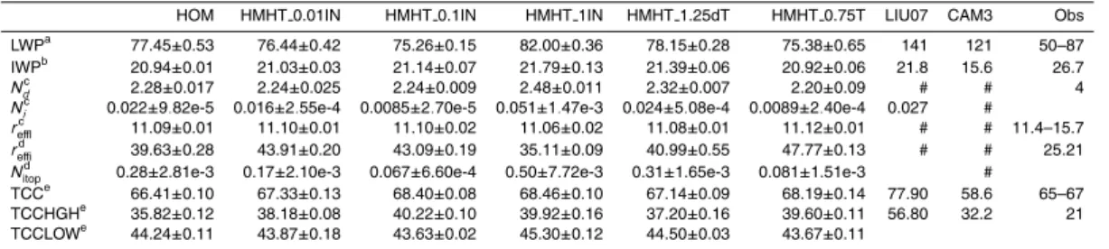
Tables 2 and 3 show the annual global mean values for several parameters in our sim-ulations along with results from the standard CAM3 and observations. The liquid water

5

path in the HOM simulation is 77 g/m2, much less than that simulated in LIU07 and in the standard CAM3, and close to the observed range of 50–84 g/m2; this value is also close to that simulated by Gettleman et al. (2008) in a modified version of CAM3 that also includes a two moment cloud microphysics treatment (74 g/m2). The large decrease in liquid water path compared with that in LIU07 is mainly caused by the

10

treatment of the Bergeron-Findeisen process where ice crystals grow at the expense of liquid droplets. As noted above, this treatment has been changed to that of Xie et al. (2008). In the treatment here, a direct conversion from liquid to ice is assumed and the in-cloud vapor pressure that is used to calculate the vapor deposition on ice crystals is the saturation vapor pressure over liquid and ice with each weighted by the

15

proportions of ice and liquid water mass (Xie et al., 2008). In LIU07, the conversion occurs as a result of supersaturation with respect to ice, where the grid-averaged va-por pressure is used to calculate vava-por deposition based on Rotstayn et al. (2000). Then the remaining liquid water is evaporated because of subsaturation with respect to liquid water, and further deposition on ice takes place. Because grid-averaged

va-20

por pressure is usually less than the saturation vapor pressure that is weighted by the proportion of ice and liquid water mass, the treatment in LIU07 results in a smaller conversion rate from liquid to ice in mixed-phase clouds than that used in this study (Xie et al., 2008; Appendix B). Because ice crystals are more e_fficient at producing precipitation, the inclusion of this process in the manner outlined here decreases the

25

liquid water path significantly compared to that in LIU07.

(22)

ACPD

9, 16607–16682, 2009

Title Page

Tables Figures

◭ ◮

Back Close

Full Screen / Esc

radius) are estimated as seen by satellite instruments using a modification of the max-imum/random cloud overlap assumption that is used in the radiative transfer calcu-lations in the NCAR CAM3 (Collins et al., 2001) to obtain the two-dimensional field (Quaas et al., 2004). Cloud top quantities are sampled only for clouds with optical depth larger than 0.3, and are also only sampled once per day at the over pass time

5

of MODIS Aqua satellite (01:30 p.m., local time). For cloud droplet radius, the samples are limited to warm clouds (cloud top temperature larger than 273.16 K), and for ice crystal radius, the samples are limited to cold cirrus clouds (cloud top temperature less than 238.16 K). Using this procedure, our simulated cloud top droplet e_ffective radius for warm clouds (cloud top temperature>273.16 K) is 11.1µm, which matches well

10

with AVHRR observations (11.40µm), but is lower than that from MODIS observations (15.7µm). The column integrated droplet number concentration averaged over 50◦S– 50◦N is 2.3_×1010m−2, and is underestimated compared with AVHRR observations (4.0_×1010m−2).

The ice water path is 21 g/m2, which is comparable to satellite observations (Fig. 18

15

in Waliser et al., 2009). The column integrated ice crystal number concentration is about 0.022_×1010m−2, which is much smaller than that predicted by Lohmann et al. (2007) (0.1–0.7_×1010m−2). The large di_fference mainly comes from the di_fference in the treatments of mixed-phase clouds. In our model, deposition/condensation freez-ing and contact freezfreez-ing are included in mixed-phase clouds. Deposition/condensation

20

freezing is parameterized based on Meyers et al. (1992) and is a function of ice su-persaturation. Mineral dust particles are the only contact freezing ice nuclei. The simulated ice crystal number concentration in mixed-phase clouds is generally less than 1/L, which compares well with observations from the M-PACE field experiments. In Lohmann et al. (2007), both mineral dust and soot particles act as contact freezing

25

(23)

ACPD

9, 16607–16682, 2009

Title Page

Tables Figures

◭ ◮

Back Close

Full Screen / Esc

simulated much higher ice crystal number concentrations than that simulated here for mixed-phase clouds. The average cloud top ice crystal radius for cold cirrus clouds (cloud top temperature less than₋35◦C) is 39.6µm, larger than that observed in the MODIS satellite (25.21µm).

Total cloud fraction is 66% which compares well with the observations. The new

cir-5

rus cloud scheme simulates significantly fewer high clouds than LIU07 and improves the model results compared with observations. Shortwave cloud forcing is₋52 W/m2, which is comparable to ERBE (₋54 W/m2) and CERES (₋47 W/m2) observations. Long wave cloud forcing is 28 W/m2, which is also comparable to ERBE (30 W/m2) and CERES (29 W/m2) observations. The precipitation rate is 2.89 mm/day, slightly higher

10

than observations.

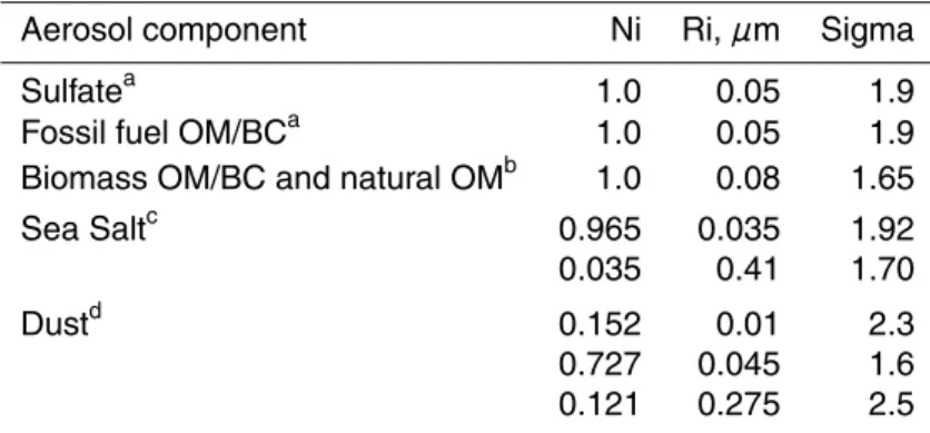
Figure 1 shows the annual average zonal mean liquid water path, ice water path, cloud top in-cloud droplet number concentration and droplet effective radius for liquid clouds, cloud top in-cloud ice crystal number and e_ffective radius for cirrus clouds (for cloud top temperatures less than₋35◦C), shortwave cloud forcing, and longwave cloud

15

forcing. Cloud top droplet number concentrations have a strong north-south contrast with a larger number concentrations in the NH, which is consistent with data derived from MODIS observations (Quaas et al., 2006), and is mainly caused by anthropogenic aerosols in the model. Correspondingly, cloud top droplet effective radius has a larger value in the SH than in the NH, which is consistent with the AVHRR observations (Han

20

et al., 1994). Liquid water path has larger values in the middle latitude storm tracks over both hemispheres, which is consistent with SSM/I data (Ferraro et al., 1996). The ice water path has two peak values in the middle latitudes of both hemispheres, which is consistent with ISCCP observations (Storelvmo et al., 2008). For cirrus clouds, cloud top ice crystal number concentration is large over the tropics and the two polar

25

(24)

ACPD

9, 16607–16682, 2009

Title Page

Tables Figures

◭ ◮

Back Close

Full Screen / Esc

forcing have latitudinal variations that agree with the CERES observations.

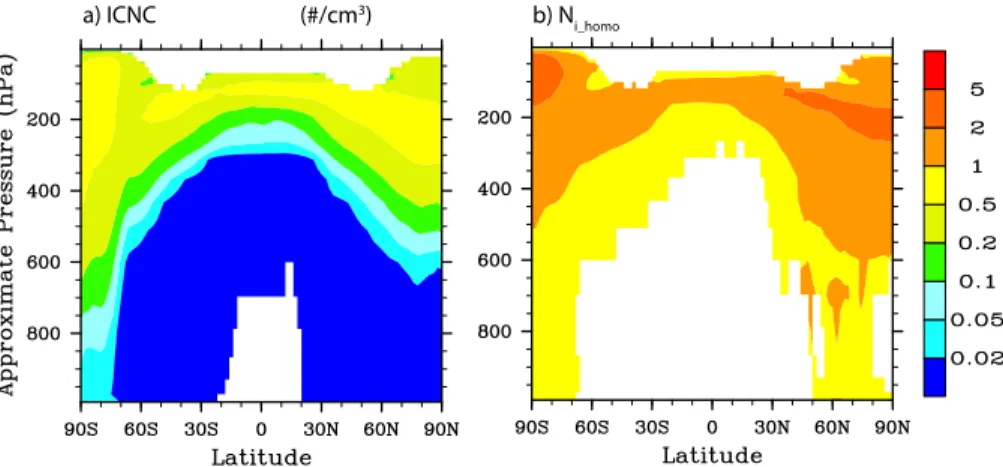
Figure 2 shows annual average zonal mean latitude-pressure cross sections for grid-averaged droplet number concentration, liquid water content, ice crystal number con-centration, and ice water content. Liquid water content shows two peaks in the storm tracks of both hemispheres, which extend into the middle troposphere. Liquid droplet

5

number concentrations show a similar pattern: two peaks in the middle latitudes in both hemispheres, but the influence of anthropogenic aerosols is also evident: there is a stronger peak in the NH than in the SH. For ice clouds, large ice crystal number con-centrations are found over the upper troposphere in tropical regions and at both poles. The simulated grid mean ice crystal number concentrations are comparable to results

10

from Lohmann et al. (2007), except that they simulated higher ice crystal number con-centrations in mixed-phase clouds, as mentioned above. Large ice water content can be found in the lower troposphere over high latitudes in both hemispheres and in the upper troposphere in the tropics.

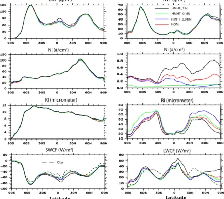
Ice water content (IWC) in the upper troposphere is compared with that from the

15

Microwave Limb Sounder (MLS) onboard the Aura Satellite (Wu et al., 2006) in Fig. 3. The MLS ice water content data have a vertical resolution of_∼3.5 km and a horizontal resolution of_∼160 km for a single MLS measurement along an orbital track (Wu et al., 2006, 2009). The data used here for comparison are monthly means from September 2004 to August 2005. The model broadly captures the spatial and zonal distribution of

20

ice water content in the upper troposphere, but it underestimates the ice water content in tropical regions by a factor of 2 to 4, which is also true for the standard CAM3 model (Li et al., 2005). The model ice water content is larger at the poles than in MLS data, a feature that is improved when heterogeneous IN are included in the model (see Sect. 4.1.2). We notice that the ice water content simulated in LIU07 is larger in

25

(25)

ACPD

9, 16607–16682, 2009

Title Page

Tables Figures

◭ ◮

Back Close

Full Screen / Esc

addition, we apply a mean vertical velocity rather than a PDF of vertical velocities, and anvil cloud fraction is added as one source term in the predicted total cloud fraction using Eq. (14) while in LIU07 the total cloud fraction is the sum of the diagnostic large scale cloud fraction and the anvil cloud fraction. These differences make it difficult to attribute di_fferences in the simulated ice water content between this study and that in

5

LIU07 to any of the individual processes. Increasing the temperature variations in our treatment, as is done in Sect. 4.2, does not alleviate this problem.

Figure 4 shows annual average zonal mean latitude-pressure cross sections for the in-cloud ice crystal number concentration from the prognostic ice crystal equation and that simulated immediately after the initial ice nucleation. Ice crystal number

concen-10

tration from the initial nucleation of ice ranges from 0.5 to 5 cm−3, and slowly increases with decreasing temperature although at very low temperatures it decreases with de-creasing temperature (Compare temperature in Fig. 2 withN_i _homoin Fig. 4b). The de-crease is caused by the low vertical velocity we used at low temperatures (Sect. 2.2). In our treatment, mean vertical velocities linearly decrease from 23 cm/s at 238 K to

15

1.2 cm/s at 193 K. Based on the homogeneous freezing parameterization of Liu and Penner (2005), ice crystal number concentration from homogeneous freezing is then at its maximum at around 200 K, which explains why ice crystal number concentration decreases with decreasing temperature at very low temperature (lower than 200 K). The ice crystal number concentrations predicted from the prognostic ice crystal

equa-20

tion are lower by a factor of 2 to 5 compared to the initial concentrations predicted after ice nucleation, due to the impact of sublimation, gravitational settling, precipitation re-moval, and advection. As shown later in Sect. 4, different freezing mechanisms lead to di_fferent ice crystal number concentrations in the upper troposphere.

Table 4 compares the simulated ice crystal number concentration from the

prognos-25

(26)

ACPD

9, 16607–16682, 2009

Title Page

Tables Figures

◭ ◮

Back Close

Full Screen / Esc

NH (Scotland, in September/October). Most flight patterns during the campaign were designed to probe young cirrus clouds (K ¨archer and Str ¨om, 2003). The measured ice crystal number concentrations in the SH and NH have a median of 1.4 and 2.2 cm−3, respectively (Gayet et al., 2004). Simulated mean ice crystal number concentrations from the prognostic ice crystal equation in the HOM case are 0.34 and 0.33 cm−3 in

5

the SH and NH, respectively, and are significantly lower than those observed during the INCA campaign. The INCA observations mainly represented young cirrus clouds, however, and ice crystal number concentrations immediately after the initial ice nu-cleation from homogeneous freezing (shown in the parenthesis for the HOM case in Table 4), are 1.2 and 1.6 cm−3in the SH and NH, respectively, in better agreement with

10

the INCA observations.

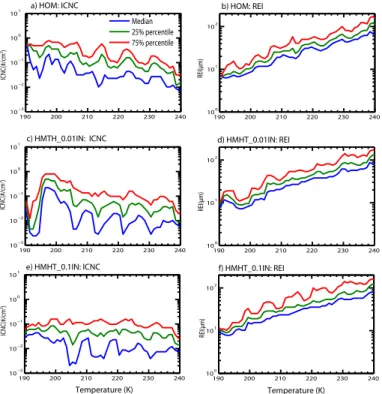
Figure 5 shows in-cloud ice crystal number concentration (ICNC) and ice crystal effective radius (REI) versus temperature. Model results are sampled every six hours over six flight regions (Kiruna, Sweden in January and February; Hohn, Germany in November and December; Forli, Italy in Octorber; Mahe, Seychelles, in February and

15

March; Darwin, Australia, in November; Aracabuta, Brazil in January and February) where the observations reported in Kr ¨amer et al. (2009) were collected (See Table 3 in Kr ¨amer et al. (2009) for the flight information). The median, 25% percentile, and 75% percentile are shown for each 1 K temperature bin. In-cloud ice crystal number concentrations in the HOM case increase with decreasing temperature (the median ice

20

crystal number concentration is 0.08 cm−3at 230 K and 0.13 cm−3at 200 K), although the vertical velocities used in the model decrease with decreasing temperature. In Kr ¨amer et al. (2009) (Fig. 9 in their paper), ice crystal number concentration decreases with decreasing temperature, with a mean value _∼0.2 cm−3 at 230 K and _∼0.1 cm−3 at 200 K. Decreasing the vertical velocity with decreasing temperature as treated in

25

(27)

ACPD

9, 16607–16682, 2009

Title Page

Tables Figures

◭ ◮

Back Close

Full Screen / Esc

radius increases faster with temperature than that in observations.

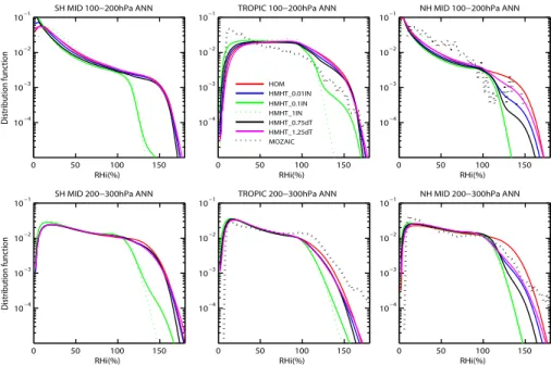
Figure 6 shows the simulated PDF of RHi outside of cirrus clouds within two layers (100–200 hPa, and 200–300 hPa) and in three regions (the SH middle latitudes: 60◦S– 30◦S; the tropics: 30◦S–30◦N; and the NH middle latitudes: 30◦N–60◦N). One year of model results are sampled every six hours. The PDF of the clear-sky RHi is calculated

5

based on the clear-sky mean RHi and the prescribed temperature perturbations used in the model (Sect. 2.2, Eq. A2) weighted by the clear sky fraction (1₋a). Also shown in Fig. 6 is the PDF of RHi from the Measurement of Ozone and Water Vapor by Airbus In-service Aircraft (MOZAIC) campaign (Spichtinger et al., 2004) for the NH middle latitudes and the tropics. MOZAIC data sampled both clear sky and cloudy

10

sky conditions. We only compared the RHi in clear sky conditions because the model assumes a uniform distribution for the in-cloud specific humidity and the large time step used in the GCM makes the saturation ratio under cloudy sky conditions very close to 1. In the clear sky, the RHi are sampled across the whole PDF spectrum regardless of whether the value of RHi exceeds the heterogeneous freezing or homogeneous

15

freezing threshold. By doing this, the in-cloud conditions sampled in the MOZAIC data are partly taken into account in the model data.

The homogeneous freezing-only case (HOM) reproduces the shape of the PDF of RHi from MOZAIC data well. RHi in the range from 20–100% occurs with large fre-quency, and the frequency has an almost exponential decay from RHi=100% to around

20

RHi=150%, a feature that is consistent with the MOZAIC data and is believed to be mainly caused by temperature variations (K ¨archer and Haag, 2004). Beyond 150%, the HOM case simulates a faster decay of RHi than that in the MOZAIC data. This fast decay in the HOM case is caused by homogeneous ice freezing that has a threshold RHi near 150%.

25

(28)

ACPD

9, 16607–16682, 2009

Title Page

Tables Figures

◭ ◮

Back Close

Full Screen / Esc

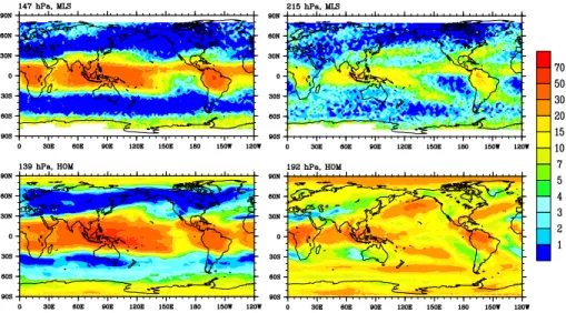
frequency of occurrence of ice supersaturation for a given grid point is calculated as the number of samples with RHi >100% divided by the total number of samples for a given period (one year in the model, September 1991 to June 1997 for the MLS data), weighted by the clear sky fraction (1₋a). In contrast to the comparison with the MOZAIC data, the mean clear-sky RHi instead of the subgrid-scale RHi in the model

5

is used to calculate the ice supersaturation frequency because of the large field view of the MLS measurement (about 100_×200 km2 perpendicular and parallel to the line of sight and 3 km vertically). At the 147 hPa level, the observed ice supersaturation occurs most frequently in the tropics between 20◦S and 20◦N and over Antarctica. Compared with the MLS data, the model with only homogeneous freezing (HOM)

re-10

produces the observations well in terms of the spatial distribution, but gives a higher ice supersaturation frequency than does the MLS data.

At the 215 hPa level, the observed ice supersaturation occurs most frequently in the same regions as at the 149 hPa level, although the high frequency ice supersaturation regions also extend toward high latitudes at 215 hPa, mainly over the storm track

re-15

gions in both hemispheres. The model produces a similar spatial distribution as that in the MLS observations but with an even larger overestimation than that at 147 hPa, and the ice supersaturation regions extend even more towards high latitudes in the model. For example, the model simulates a high frequency of ice supersaturation occurrence in the SH storm track (around 45◦S), which is not present in the MLS observations. As

20

pointed out by Spichtinger et al. (2003), there are considerable data gaps in the mid-dle latitudes of the summer hemispheres in the MLS data. This may prevent us from drawing further conclusions about whether the simulated ice supersaturation regions over the storm track at the 215 hPa level is reasonable or not. To summarize the model performance regionally, averaged supersaturation frequencies in five regions (global,

25

(29)

ACPD

9, 16607–16682, 2009

Title Page

Tables Figures

◭ ◮

Back Close

Full Screen / Esc

(Sect. 4.1).

The simulated supersaturation frequencies also depend on the mesoscale tempera-ture perturbations used in the model. A large temperatempera-ture perturbation produces more ice, which decreases the clear sky relative humidity and decreases the supersatura-tion frequency simulated in the model. A larger temperature perturbasupersatura-tion, then, would

5

improve the comparison with MLS data, especially at 139 hPa, since quite small tem-perature perturbations were used due to the low temtem-peratures there (Sect. 2.2). Larger mesoscale temperature perturbations at higher altitude is also consistent with gravity wave theory (Fritts and Alexander, 2003) and observations (Gary et al., 2006) although larger vertical velocities resulting from larger temperature perturbations by using Eq. (2)

10

would produce high ice crystal number concentrations that are not supported by field observations, as discussed in Sect. 2.2.

4 Effects of heterogeneous IN and mesoscale temperature perturbations 4.1 Effects of heterogeneous IN

The effects of heterogeneous IN on cirrus cloud properties are studied using three

sen-15

sitivity tests: HMHT 0.01IN, HMHT 0.1IN, and HMHT 1IN, in which IN concentrations are assumed to be 1%, 10%, and 100% of the total number concentration of BC and dust particles, respectively, as described in Table 1. The annual average zonal mean distributions of dust and BC number concentrations are shown in Fig. 9. BC particles have a high concentration in the NH upper troposphere (100 hPa to 400 hPa) with a

20

range of 1–10 cm−3, caused by the larger anthropogenic emissions in the NH. The number concentrations of BC particles in the upper troposphere decrease with latitude from north to south. In the upper troposphere of the SH, the concentrations range from 0.3 to 1 cm−3. Dust particles are much lower in number concentration and there is a stronger gradient with altitude from the surface to the upper troposphere than for

25