On the distribution of relative humidity in cirrus clouds

(1)

ACPD

4, 365–397, 2004

Relative humidity in cirrus clouds

P. Spichtinger et al.

Title Page

Abstract Introduction

Conclusions References

Tables Figures

◭ ◮

Back Close

Full Screen / Esc

Print Version Interactive Discussion

©EGU 2004 Atmos. Chem. Phys. Discuss., 4, 365–397, 2004

www.atmos-chem-phys.org/acpd/4/365/ SRef-ID: 1680-7375/acpd/2004-4-365 © European Geosciences Union 2004

Atmospheric Chemistry and Physics Discussions

On the distribution of relative humidity in

cirrus clouds

P. Spichtinger1, K. Gierens1, H. G. J. Smit2, J. Ovarlez3, and J.-F. Gayet4

1

Deutsches Zentrum f ür Luft- und Raumfahrt, Institut f ür Physik der Atmosph äre, Oberpfa_ffenhofen, Germany

2

Forschungszentrum J ülich, Institut f ür Chemie und Dynamik der Geosph äre (ICG-II: Troposph äre), J ülich, Germany

3

Laboratoire de M ´et ´eorologie Dynamique du CNRS, Ecole Polytechnique, Palaiseau, France

4

(2)

ACPD

4, 365–397, 2004

Title Page

Tables Figures

◭ ◮

Back Close

Full Screen / Esc

©EGU 2004

Abstract

We have analysed relative humidity statistics from measurements in cirrus clouds taken unintentionally during the Measurement of OZone by Airbus In-service airCraft project (MOZAIC). The shapes of the in-cloud humidity distributions change from nearly sym-metric in relatively warm cirrus (warmer than−40◦C) to considerably positively skew

5

(i.e. towards high humidities) in colder clouds. These results are in agreement to find-ings obtained recently from the INterhemispheric differences in Cirrus properties from Anthropogenic emissions (INCA) campaign (Ovarlez et al.,2002). We interprete the temperature dependence of the shapes of the humidity distributions as an effect of the length of time a cirrus cloud needs from formation to a mature equilibrium stage,

10

where the humidity is close to saturation. The duration of this transitional period in-creases with decreasing temperature. Hence cold cirrus clouds are more often met in the transitional stage than warm clouds.

1. Introduction

The formation of cirrus clouds in the upper troposphere requires that the relative

hu-15

midity (with respect to ice,RHi) exceeds certain freezing thresholds. These are gener-ally much higher than 100%; for instance, homogeneous freezing of aqueous solution droplets at temperatures below the supercooling limit of pure water (≈ −40◦C) needs RHi > 140% (Koop et al.,2000). Cirrus formation and its subsequent evolution into a mature cirrus cloud (whereRHi is close to saturation) a_ffects the ambient relative

20

humidity field, and it is possible to conclude on cirrus formation pathways by investiga-tion of their ambientRHi-distribution (Haag et al.,2003). It is obvious that the humidity within a cloud is even stronger a_ffected by the cloud since it is directly involved in the mi-crophysical processes. It is then clear that the mimi-crophysical processes within a cloud shape the statistical distribution of theRHi-field. Therefore it should principally be

pos-25

(3)

ACPD

4, 365–397, 2004

Title Page

Tables Figures

◭ ◮

Back Close

Full Screen / Esc

©EGU 2004 within clouds.

The statistical distribution of the relative humidity with respect to ice within cirrus clouds was investigated byOvarlez et al. (2002) using data obtained during the INCA campaigns in the southern (Punta Arenas, Chile, 55◦S) and northern (Prestwick, Scot-land, 55◦N) hemispheres, respectively. The distinction between in-cloud and

out-of-5

cloud situations was made on the basis of the extinction coefficient measured with a polar nephelometer (Gayet et al.,1997): An extinction coefficient of less than 0.05 km−1 was considered a cloud free situation. This corresponds roughly to an ice crystal con-centration of 50–100 particles L−1 of 5 µm diameter. Ovarlez et al. (2002) found es-sentially that two types of distributions can be well fitted to the observations. These are

10

a Gaussian distribution for cirrus warmer than−40◦C and a Rayleigh distribution for cirrus colder than−40◦C. The main point to note here is rather the symmetry of the re-spective distribution than the type of the distribution itself (which should be considered merely a convenient mathematical expression for the fits). Warmer clouds possess symmetric or quasi-symmetric distributions of RHi centred about 100% (exemplified

15

by the Gaussian) whereas colder clouds possess distributions of RHi with positive skewness (exemplified by the Rayleigh distribution), i.e. they have a tail towards higher values. This tail might be interpreted a signature of cloudsin statu nascendi, where the supersaturation has not yet relaxed to a value close to equilibrium (i.e. saturation). Ovarlez et al. (2002) found slight differences between the in-cloud humidity

distribu-20

tions obtained at the two locations, with a tendency for higher values of RHi in the southern hemisphere.

In the present paper we analyse humidity data from another data source, namely from the Measurement of OZone by Airbus In-service airCraft project (MOZAIC,Marenco et al.,1998;Helten et al.,1998) and we will show that these data are consistent with

25

(4)

ACPD

4, 365–397, 2004

Title Page

Tables Figures

◭ ◮

Back Close

Full Screen / Esc

©EGU 2004

2. Data handling

For the present investigation we use the statistical data of relative humidity with re-spect to ice in the (mostly northern hemispheric) tropopause region as obtained from MOZAIC aircraft (Gierens et al., 1999). For this data set it is not really possible to decide whether a recording that signals supersaturation comes from cloud free air or

5

from within a cirrus cloud. Thus the humidity statistics obtained from the data set bears signatures from both cloudy and clear air. Of course, data from substantially subsaturated air are obviously obtained in clear regions. The common characteristics of all humidity statistics obtained from these data sets is a relatively flat exponential distribution for the subsaturated air (i.e. 20%.RHi .80%) and a steeper exponential

10

distribution in supersaturated air masses (cf. Fig2). These characteristics can also be found in humidity statistics obtained from the microwave limb sounder (MLS) on board the Upper Atmosphere Research Satellite (UARS), where a cloud clearing could be performed successfully (Spichtinger et al.,2002,2003). Hence, the exponential parts of the humidity statistics are characteristic for cloud free air. The signature of clouds

15

in the MOZAIC data is a “bulge” around saturation (i.e.RHi ≈ 100±20%). Such a bulge is not present in the cloud cleared MLS data. Whereas we were interested in the exponential parts of the humidity statistics in our previous papers, we will here consider the “cloud bulge” in more detail.

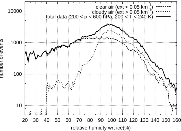
The interpretation of the bulges as a cloud signature can be underpinned by taking

20

a look at data from the INCA project, namely at the combination of humidity data from the frostpoint hygrometer (Ovarlez et al., 2002) and extinction data from the neph-elometer (Gayet et al., 1997). The combination allows to distinguish in-cloud from out-of-cloud data records: As in the work of Ovarlez et al. (2002) we fix the cloud threshold at an extinction of 0.05 km−1. Using all measurements in the pressure range

25

(5)

ACPD

4, 365–397, 2004

Title Page

Tables Figures

◭ ◮

Back Close

Full Screen / Esc

©EGU 2004 shown in Fig.1. The relative humidity distribution of cloud free data shows the usual

characteristic of tropospheric data (see e.g. Gierens et al., 1999; Spichtinger et al., 2002). The shape of the distribution can be described using two exponential distribu-tions with different slopes. As we expected, there is a kink at saturation. In contrast the distribution obtained from the cloudy data has the shape as described inOvarlez

5

et al. (2002): The distribution is centred at saturation and the frequency of occurrence of relative humidity decreases towards lower and higher humidities. The most interest-ing distribution for our present purpose is that obtained from the sum. This distribution has qualitatively the same shape as the distributions obtained from the MOZAIC data: There is the characteristic shape of the pair of exponential distributions (typically for

10

tropospheric data) but there is also a bulge around saturation. This bulge is the result of the in-cloud data which is evident from the figure.

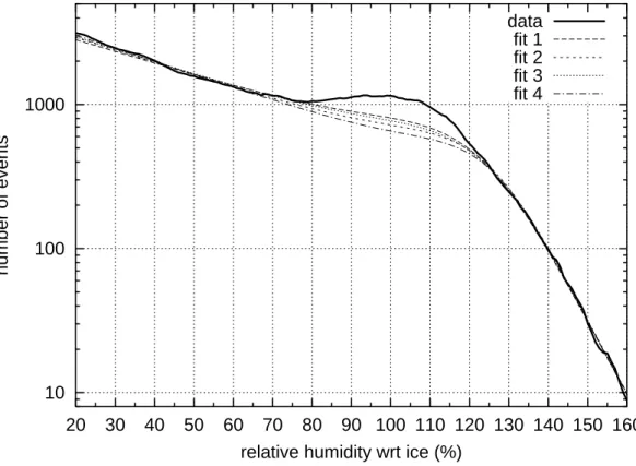
In order to investigate the cloud bulges in MOZAIC data we treat the data in the following way: First we run a moving average (with a window width of 5%RHi) over the respective distribution to reduce their statistical noise. Then we construct baselines

15

representing the exponential parts of each distribution and subtract them from their respective distribution of RHi. The residuum from this operation is the bulge alone. This baseline is constructed in the following way: On the left and the right of the bulge there are the exponentials with their different slopes (2 free parameters).These two exponentials are then smoothly connected by means of an “exponential” with varying

20

exponent. The varying exponent is a Fermi function centred at a value close to 100% (1 free parameter). The width of the Fermi function is adjustable (1 free parameter). The whole baseline function is scaled with another adjustable parameter, such that there are a total of 5 free parameters. The functional form of the baseline is then:

B(x)=Nexp[−F(x)·(x−x_c)] (1)

25

with the Fermi function

F(x)=a+ b−a

(6)

ACPD

4, 365–397, 2004

Title Page

Tables Figures

◭ ◮

Back Close

Full Screen / Esc

©EGU 2004 Obviously, the limiting values for large negative (subsaturation) and large positive

val-ues (supersaturation) ofx−xc area andb, respectively, which are the slopes of the

corresponding exponential distributions. x_c is the value where the Fermi function is centred, andcdetermines the sharpness of the transition between the two slopes a andb.Nis the scale parameter. These five free parameters ({a, b, c, xc, N}) are deter-5

mined numerically using a simple optimisation routine, that aims at minimising the sum of squared differences between the baseline fit and the data in the two RHi regions where the distribution is exponential.

After subtraction of the baseline the cloud bulge plus some residual noise remains and can be studied further. This is done in the next section. Certainly, the

remain-10

ing bulge is sensitive to the construction of the baseline and to the parameters. For studying the impact of baseline construction on the bulge we have used the following procedure: For each distribution ofRHi we have constructed several baselines distin-guished by di_fferent ranges of best fit in the exponential parts, e.g. 30–70% or 30–80% etc. The standard range for the calculations was 40–80%RHi and 120–160% RHi.

15

Within these ranges the distributions obviously follow exponential distributions. The dif-ferent fit rangesper seimply di_fferences in the goodness-of-fit measureχ2. Therefore we use for comparison of the quality of the fits a normalisedχ_RHi2 :=100%· _∆χ_RHi2 were ∆RHi denotes the range within the baseline was constructed. With this variable we are able to determine the best baseline and using the distinct baselines we can study

20

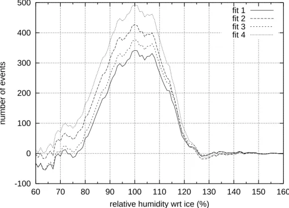
the variations of baseline construction and their impact on the bulge. An example of some di_fferent baseline fittings is given in Fig.2.

The corresponding bulges after subtraction of these various baselines are shown in Fig.3.

We interprete the bulges or the di_fference distributions as cloud signatures and as

25

(7)

ACPD

4, 365–397, 2004

Title Page

Tables Figures

◭ ◮

Back Close

Full Screen / Esc

©EGU 2004 indicates, that with the baselines subtracted we probably also remove in-cloud data,

especially in the supersaturated region. As (Fig.1) shows, the slopes of the humidity distributions above ice saturation in the in-cloud and out-of-cloud INCA data are similar, which could mean that by the baseline subtraction we remove from all supersaturation bins nearly a constant (but here unknown) fraction of in-cloud data. However, since

5

there is no possibility to flag cloudy data, we do not see a better possibility of baseline construction. Thus we have to accept that we miss some of the cloudy data and that we also have negative values in the residuals, which we will set to zero for the further analysis.

For analysis of the difference distributions we calculate the mean values, standard

10

deviations and the so-called L-skewness (for a definition see the appendix). We use the L-skewness instead of the usual skewness because of its greater robustness against outliers (see e.g.Guttman,1993), which is necessary here because there is still some noise in the bulge data even after the initial smoothing. The traditional skewness is very sensitive to such noise and can therefore not be used as a reliable measure.

15

These statistical measures are calculated in the range 70–150% RHi, which per se introduces a certain positive skewness even in a perfectly symmetric distribution (see below). The lower boundary is considered a lower threshold where most cirrus clouds will be evaporated completely. The upper boundary is a typical threshold for homogeneous ice nucleation in the upper troposphere (seeKoop et al.,2000); higher

20

thresholds apply for still colder temperatures, but the data get more noisy, hence we constrain the range for our calculations to 150% and do not go beyond. Since we constrain the calculation of mean, standard deviation and L-skewness to this range which is asymmetric with respect to saturation, we have to determine how this a_ffects in particular the calculation of the skewness. In order to estimate this effect we analyse

25

(8)

ACPD

4, 365–397, 2004

Title Page

Tables Figures

◭ ◮

Back Close

Full Screen / Esc

©EGU 2004 distribution

f_X(x)= _p1 2πσ0

exp −1 2

_x₋_µ 0 σ0

2!

is centred atµ0 = 100%RHi and the parameter σ0 = 11.25% RHi is chosen such that the standard deviation (for the range 70–150%RHi) is similar to those determined for the bulges. If we now compute the statistical measures in the restricted range

5

70–150% RHi, we find the mean value in the range 100.11 ≤ µ ≤ 100.19% RHi (the greater value arises when the noise peak at 150% is added), and the standard deviation in the range 11.10≤σ ≤11.28%RHi. The most important result is that the L-skewnessτ3 ranges within: 0.0077 ≤τ3 ≤ 0.0161 (for a symmetric distribution the L-skewness is zero by definition). Hence, in the discussion of the results a distribution

10

withτ₃≤0.0161 can be classified as nearly symmetric, a distribution withτ₃>0.0161 can be classified as asymmetric.

3. Results

3.1. MOZAIC data

Let us first consider MOZAIC data recorded south of 30◦N (tropical data) between

15

1995 and 1999. We show tropospheric data from four pressure levels 190–209, 210– 230, 231–245, and 246–270 hPa (hereafter levels 1–4). All these are characterised by a rather narrow temperature distribution. The mean temperatures on the four lev-els are −54,−49,−44, −39◦C, respectively, the standard deviations range between 2.0◦C and 3.3◦C. Hence, using these levels there is a splitting of the data in distinct

20

(9)

ACPD

4, 365–397, 2004

Title Page

Tables Figures

◭ ◮

Back Close

Full Screen / Esc

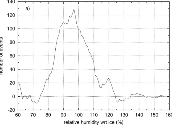
©EGU 2004 the variations of the baseline fits, particularly the varying L-skewness. The measured

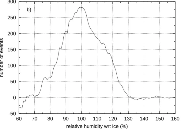
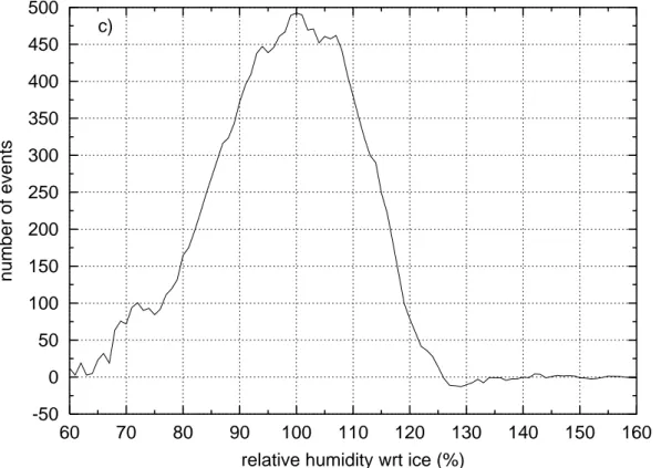
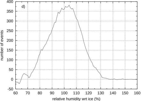
humidity distributions of the cloud bulges (after baseline subtraction of the best fit, i.e. minimisingχ_RHi2 ) are presented in Fig.4.

It can be seen that after baseline subtraction the residual number of events is rather small compared to the original data base (cf. the numbers along the y-axis of Fig.2).

5

But nevertheless, the distributions contain a considerable fraction of the total data (13– 33%, depending on the pressure level) and the noise in the distributions is quite small (due to the moving average of theRHi-distributions). For all distributions we see quite the same shape: The distribution is centred around saturation, the mean values range between 97 and 103%RHi and the standard deviations are about 11% RHi (see

Ta-10

ble 1). The di_fference distributions obtained at the two upper pressure levels (level 1 and 2) are clearly skew (i.e. asymmetric), distributions from the two lower levels (level 3 and 4) are symmetric. This result can be verified by the L-skewness: For the two upper pressure levels the L-skewness τ3 takes values in the following intervals: 0.1068 ≤ τ3(level 1) ≤0.1310 and 0.0071 ≤ τ3(level 2) ≤ 0.0598. Hence, the diff

er-15

ence distributions for the upper two levels are asymmetric according to the L-skewness (see Sect. 2). For the two lower pressure levels the L-skewness τ3 ranges between −0.0480 and 0.0084, therefore we can assume that the distributions are nearly sym-metric according to the L-skewness (see Sect.2).

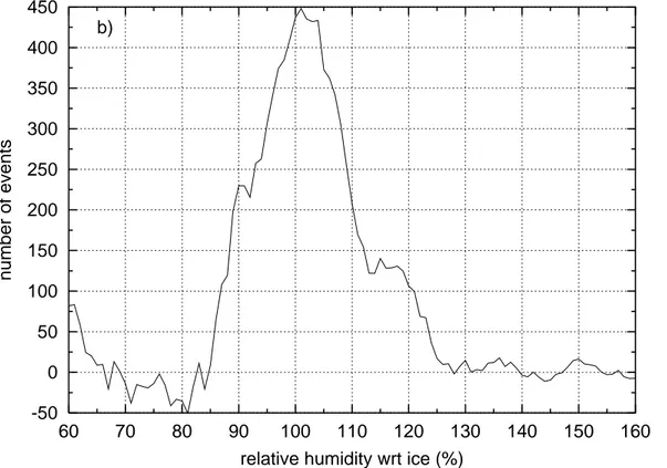
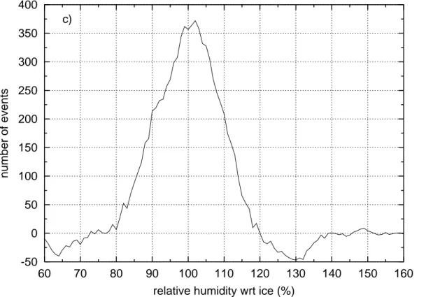
We now consider tropospheric MOZAIC data recorded north of 30◦N (extratropical

20

data) between 1995 and 1999 in the pressure range 175≤p≤275 hPa. For this data set there is not such a sharp temperature stratification due to the pressure levels as in the tropical data. Hence, for studying the distributions in distinct temperature classes we split the data in the following way: One classK1contains all data with temperatures in the interval−55 ≤ T ≤ −50◦C, and one class K2 with temperatures in the interval

25

(10)

ACPD

4, 365–397, 2004

Title Page

Tables Figures

◭ ◮

Back Close

Full Screen / Esc

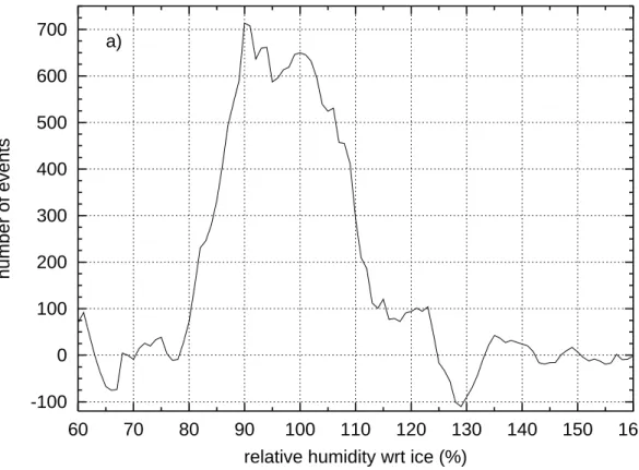
©EGU 2004 As for the tropical data after baseline subtraction the residual number of events is

rather small compared with the original data set. But also in these cases the remaining number of data in the difference distributions are large enough to draw some conclu-sions although the fraction of the remaining data ranges between 2 and 8%: The total number of data are much higher for the extratropics than for the tropics. The statistical

5

noise is quite small again.

We can see a similar result as for the tropical distributions: the difference distributions for the three data classes are again centred at saturation, the mean values range between 98 and 106%RHi, the standard deviations range between 8 and 11%RHi.

The difference distributions obtained from the total extratropic data and the “cold

10

data” are clearly skew, the distribution obtained from the “warm data” is almost sym-metric. This is confirmed by the L-skewnesses: For the total data the L-skewness is 0.0955 ≤ τ3 ≤ 0.1178, for the “cold data” the L-skewness is 0.0882 ≤ τ3 ≤ 0.1225. Hence, these distributions are clearly asymmetric. The L-skewness for the “warm data” is−0.0186≤τ3≤0.0524 and therefore we can conclude, that this distribution is almost

15

symmetric.

The mean values, standard deviations and L-skewness values are collected in Ta-ble1, the L-skewness values (and their variations) are visualised in Fig.6. In this figure additionally the values for a Gaussian distribution and a perturbed Gaussian distribu-tion (see Sect.2) are shown, hence it is easy to distinguish between the symmetric and

20

asymmetric distributions.

In looking at Fig. 6 one should consider the values displayed as lower estimates, because, as stated before, the range of the computation of the moments was confined at 150% RHi and cloud events can get lost in our baseline subtraction procedure. Since this happens evidently more probably in the supersaturated than in the

subsatu-25

(11)

ACPD

4, 365–397, 2004

Title Page

Tables Figures

◭ ◮

Back Close

Full Screen / Esc

©EGU 2004 3.2. INCA data

The INCA campaigns took place in the extratropical latitudes of both hemispheres. Hence, we can compare the distributions of relative humidity in clouds obtained from the INCA data set to the corresponding distributions obtained from the extratropical MOZAIC data. As before we have picked the INCA data out of two different temperature

5

classes: The classC1contains all data in the temperature range−55≤T ≤ −50

◦

C and the classC2contains all data in the temperature range−50≤T ≤ −45

◦

C. For these two classes we have calculated the L-skewness in the range 70–150%RHi. The values for the two distributions (τ₃(C₁) = 0.1377, τ₃(C₂) = 0.0860) are visualised in Fig. 6. We get the same qualitative effect as for the two difference distributions obtained from

10

the temperature classes K1 and K2 (MOZAIC): For the colder clouds the distribution is skewer than for the warmer clouds. Comparing these values with the L-skewness obtained from the MOZAIC data (classesK1andK2) we see that the values of MOZAIC data are a lower approximation due to the causes mentioned in Sect.2.

3.3. MLS data

15

In order to show as a contrast to the previous data sets an example where cloud clear-ing works effectively, we show here one example of MLS data analysis for the two nom-inal pressure levels of 147 hPa and 215 hPa (Spichtinger et al.,2002,2003). Figure7 shows that for all concerned tropospheric data sets after baseline subtraction there re-mains only noise. This can be interpreted that the cloud clearing algorithm described

20

inSpichtinger et al.(2002,2003) works very well and almost no cloudy measurements are left in the data.

4. Discussion

Obviously there is a qualitative difference between the in-cloud distributions ofRHi for warm and cold cirrus, respectively. This contrast consists of the di_fferent shapes of the

(12)

ACPD

4, 365–397, 2004

Title Page

Tables Figures

◭ ◮

Back Close

Full Screen / Esc

©EGU 2004 distributions, namely symmetric for warm cirrus versus positively skew for cold cirrus.

This leads to the question about the physical processes (or possibly selection biases) that produce such qualitatively different distributions of in-cloud relative humidity.

We believe that the difference we see in the humidity distributions is caused by the temperature dependence of the length of time a cirrus cloud needs to approach

sat-5

uration from an initial high supersaturation at its instant of formation. This transitional period is about twice as long at−60◦C than at −40◦C, because both the diffusivity of water molecules in air and the saturation vapour pressure decrease with decreasing temperature. The nominal crystal growth time scale in a young cirrus cloud can be written as (Gierens,2003)

10

τ_g =7.14×105T−1.61_p_[s

0e∗(T)]−1/3N−2/3, (3) with initial supersaturation at cirrus formations0, saturation vapour pressure over ice e∗(T) (in Pa), and number density of ice crystals formed N (in m−3). τ_g is in sec-onds. Typical growth time scales range from 10 min to half an hour, however, the cirrus transition time to phase equilibrium is more than double that quantity, in particular

be-15

cause initially the condensation rate is very small since the ice crystals are very small. This means that the transition period from cirrus formation to phase equilibrium can make up a substantial fraction of the total cloud life time. In fact, especially thin and sub-visible cirrus in cold air (below about 215 K) may not reach equilibrium at all, i.e. the crystals sediment out of the cloud before the in-cloud humidity reaches saturation

20

(K ¨archer, 2002). This in turn implies that a substantial fraction of the cirrus clouds probed unintentionally by a MOZAIC aircraft can still be in the transition phase. Since the duration of the transition phase increases with decreasing temperature, the proba-bility to probe a cirrus in the transition phase instead of the equilibrium phase increases with decreasing temperature. From this consideration we would expect, that we find

25

(13)

ACPD

4, 365–397, 2004

Title Page

Tables Figures

◭ ◮

Back Close

Full Screen / Esc

©EGU 2004 additionally leads to a longer relaxation phase for cold than for warm clouds.

Also vertical motions have an influence on the duration of the transition to phase equilibrium. Uplifting motions evidently prolong this period. The effect can be quantified by using the updraft time scale,τ_u (Gierens,2003):

τu =1.67×10−2w−1T2, (4)

5

with vertical velocity w. The transition duration increases with decreasing updraft timescale. Hence, strong vertical motion leads to an additional prolongation of the transition period. Unfortunately, the MOZAIC data base contains no information about vertical velocities, therefore this effect cannot be quantified. Additionally, at the same vertical motion the transition duration increases with decreasing temperature, which

10

adds to the microphysical temperature effect mentioned above.

We have performed a simple numerical exercise to simulate the transition process without considering the dynamical effect. The simulation starts with an initial relative humidity of 140% or 160%, and then theRHi changes in variable steps of about±1% according to the sign of a uniformly distributed random number. The range of the

15

random number distribution is slightly asymmetric around zero such that there is always a slightly higher chance thatRHi gets closer to 100% than further away. The number of steps is 800 for representation of a cold case, which is a suffiently small number that the system has still a memory of its initial state, that is, it is in a transitional stage. In this case the initial relative humidity was set to 160%RHi. For the warm case we use

20

1600 steps (i.e. 2×800, since one step in the cold case represents about double the time of one step in the warm case, because of the different growth time scales, see above). It turns out that this number of steps is sufficient to loose the memory of the initial state. In this case the initial relative humidity was set to 140%RHi. In order to get smooth statistics, this simulation is repeated 100 000 times for each case. We find

25

(14)

ACPD

4, 365–397, 2004

Title Page

Tables Figures

◭ ◮

Back Close

Full Screen / Esc

©EGU 2004 a considerable tail in theRHi-distribution extending to the initial value of 160%. The

L-skewness values of the two simulations are indicated in Fig. 6 as crosses. Hence, the values are similar to the values obtained from the difference distributions of the different data sets. For the skewness of the distributions the main impact is due to the number of steps, i.e. the di_fferent growth time. The initial relative humidity only slightly

5

affects the skewness.

Having the INCA data it is the relatively straightforward idea to apply the baseline fitting and subtraction also to this data set and to compare the resulting cloud bulge with the true in-cloud distribution of relative humidity (dotted curve in Fig.1). Although the amount of INCA data is not sufficient to perform the complete analysis (too much

10

noise!) this test gives interesting results. First, we find that the residual number of events (i.e. the cloud bulge) only represents about 1/5 to 1/4 of the true cloud events found by the nephelometer analysis. Such a fraction might be expected to be char-acteristic for the MOZAIC data as well. However, the INCA derived fraction cannot be generalised to MOZAIC in a straightforward way because of different measurement

15

strategies, techniques, and hence different selection biases. Second, the out of cloud data in Fig.1 (dashed curve) can be fitted with a baseline function very well over the total range from 30 to about 150%RHi (not shown), since it does not display a bulge around saturation. This means that clouds thinner than the nephelometer threshold do not contribute much to a bulge signature, and that the bulge mainly represents thicker

20

clouds. TheRHi-statistics within thin clouds therefore seems to resemble that of clear air which can result because the relaxation time for thin clouds can be extremely long (N small in Eq. 3). It can even be longer than the sedimentation time scale for the ice crystals; such clouds do not reach phase equilibrium at all (cf.K ¨archer,2002).

5. Conclusions

25

(15)

ACPD

4, 365–397, 2004

Title Page

Tables Figures

◭ ◮

Back Close

Full Screen / Esc

©EGU 2004 where RHi is distributed exponentially, and the residuals after baseline subtraction

have been investigated. The residuals, interpreted as data stemming from measure-ments within cirrus clouds, are unimodal distributions peaked close to saturation, with standard deviations of the order 10% in relative humidity units. The interpretation of the residuals as cloud signatures is corroborated by corresponding features in the INCA

5

data, where clouds can be detected using nephelometer data.

As in the earlier work of Ovarlez et al. (2002) the shape of the residual distribu-tions (the cloud bulge) turned out to depend on cloud temperature. Whereas we found nearly symmetric distributions in warm cirrus (T > −40◦C), the distributions are clearly positively skew in colder clouds. The skewness seems to increase with decreasing

10

temperature.

Our interpretation of this feature is that warm cirrus clouds probed unintentionally by MOZAIC aircraft are mostly in a mature stage. The signature of this is a symmetric distribution ofRHi centred at saturation. On the other hand, cold cirrus probed unin-tentionally are more often in a transitional state between their instant of formation and

15

their mature stage. The signature of the transitional stage is a tail in the distribution extending from saturation to the threshold relative humidity for freezing. The origin of the difference lies in the different lengths of time a cirrus needs to reach equilibrium via crystal growth after its formation at high supersaturation. The growth time scale decreases with decreasing temperature, such that the time of transition is about twice

20

as long at−60◦C than at−40◦C. This difference is reflected in the different shapes of the humidity distributions within clouds.

Appendix: L-moments

Formal definition of L-moments:

25

For this purpose one uses sample probability weighted momentsbr (r =0,1,2,3. . .).

(16)

or-ACPD

4, 365–397, 2004

Title Page

Tables Figures

◭ ◮

Back Close

Full Screen / Esc

©EGU 2004 der, are given by

b0:= 1 n

n

X

j=1

Xj (5)

br:=

1 n

n

X

j=r+1

(j−1)(j−2). . .(j−r)

(n−1)(n−2). . .(n−r)Xj. (6)

Using these weighted momentsb_r in combination with the coefficients of the “shifted Legendre polynomials” one can define the so-called L-moments:

5

l1:=b0 (7)

l2:=2b1−b0 (8)

l3:=6b2−6b1+b0 (9)

.. .

By combining these L-moments we can calculate some robust analoga to the usual

10

higher moments in statistics (e.g. skewness or kurtosis). For our purpose only the L-skewness is important:

L-skewness τ3:= l3 l2

. (10)

For calculating the L-skewness we use the method ofHosking(1990) which is based on order statistics.

15

(17)

ACPD

4, 365–397, 2004

Title Page

Tables Figures

◭ ◮

Back Close

Full Screen / Esc

©EGU 2004

References

Gayet, J.-F., Cr ´epel, O., Fournol, J. F., and Oshchepkov, S.: A new airborne polar Nephelometer for the measurement of optical and microphysical cloud properties. Part I: Theoretical design, Ann. Geophys. 15, 451–459, 1997. 367,368

Gierens, K.: On the transition between heterogeneous and homogeneous freezing, Atmos.

5

Chem. Phys., 3, 437–446, 2003. 376,377

Gierens, K., Schumann, U., Helten, M., Smit, H. G. J., and Marenco, A.: A distribution law for relative humidity in the upper troposphere and lower stratosphere derived from three years of MOZAIC measurements. Ann. Geophys. 17, 1218–1226, 1999. 368,369

Guttman, N. B.: The use of L-moments in the determination of regional precipitation climates,

10

J. Climate, 6, 2309–2325, 1993. 371

Haag, W., K ¨archer, B., Str ¨om, J., Minikin, A., Lohmann, U., Ovarlez, J., and Stohl, A.: Freezing thresholds and cirrus cloud formation mechanisms inferred from in situ measurements of relative humidity, Atmos. Chem. Phys., 3, 1791–1806, 2003. 366

Helten, M., Smit, H. G. J., Str ¨ater, W., Kley, D., Nedelec, P., Z ¨oger, M., and Busen, R.:

Calibra-15

tion and performance of automatic compact instrumentation for the measurement of relative humidity from passenger aircraft, J. Geophys. Res., 103, 25 643–25 652, 1998. 367

Hosking, J. R. M.: L-moments: analysis and estimation of distributions using linear combina-tions of order statistics, J. R. Stat. Soc., Series B, 52, 105–124, 1990. 380

K ¨archer, B.: Properties of subvisible cirrus clouds formed by homogeneous freezing, Atmos.

20

Chem. Phys., 2, 161–170, 2002. 376,378

Koop, T. Luo, B. Tsias, A., and Peter, T.: Water activity as the determinant for homogeneous ice nucleation in aqueous solutions, Nature, 406, 611–614, 2000. 366,371

Marenco, A., Thouret, V., Nedelec, P., Smit, H., Helten, M., Kley, D., K ¨archer, F., Simon, P., Law, K., Pyle, J., Poschmann, G., von Wrede, R., Hume, C., and Cook, T.: Measurement of ozone

25

and water vapor by Airbus in-service aircraft: The MOZAIC airborne program, an overview, J. Geophys. Res., 103, 25 631–25 642, 1998. 367

Ovarlez, J., Gayet, J.-F., Gierens, K., Str ¨om, J., Ovarlez, H., Auriol, F., Busen, R., and Schu-mann, U.: Water vapor measurements inside cirrus clouds in northern and southern hemi-spheres during INCA, Geophys. Res. Lett., 29, doi:10.1029/2001GL014440, 2002. 366,

30

367,368,369,379

(18)

ACPD

4, 365–397, 2004

Title Page

Tables Figures

◭ ◮

Back Close

Full Screen / Esc

©EGU 2004 the global tropopause region, Meteorol. Z., 11, 83–88, 2002. 368,369,375

(19)

ACPD

4, 365–397, 2004

Title Page

Tables Figures

◭ ◮

Back Close

Full Screen / Esc

©EGU 2004

Table 1. Variations of mean values, standard deviations and L-skewness for the difference

distributions of the different MOZAIC data sets for distinct baseline fits as described in Sect.2.

data µ(%RHi) σ(%RHi) τ₃

tropical

lev. 1 96.86–99.88 10.18–10.50 0.1068–0.1310 lev. 2 97.56–102.96 10.60–12.14 0.0071–0.0598 lev. 3 98.39–100.95 10.22–11.69 –0.0480–0.0084 lev. 4 100.87–101.48 10.71–12.28 –0.0068–0.0057 extratr.

(20)

ACPD

4, 365–397, 2004

Title Page

Tables Figures

◭ ◮

Back Close

Full Screen / Esc

©EGU 2004

10 100 1000 10000

20 30 40 50 60 70 80 90 100 110 120 130 140 150 160

number of events

relative humidty wrt ice(%)

clear air (ext < 0.05 km-1) cloudy air (ext > 0.05 km-1) total data (200 < p < 600 hPa, 200 < T < 240 K)

Fig. 1. Statistical distributions (non-normalised) of relative humidity wrt ice inside (dashed

(21)

ACPD

4, 365–397, 2004

Title Page

Tables Figures

◭ ◮

Back Close

Full Screen / Esc

©EGU 2004

10 100 1000

20 30 40 50 60 70 80 90 100 110 120 130 140 150 160

number of events

relative humidity wrt ice (%)

data fit 1 fit 2 fit 3 fit 4

(22)

ACPD

4, 365–397, 2004

Title Page

Tables Figures

◭ ◮

Back Close

Full Screen / Esc

©EGU 2004

-100 0 100 200 300 400 500

60 70 80 90 100 110 120 130 140 150 160

number of events

fit 1 fit 2 fit 3 fit 4

Fig. 3. Examples of the remaining bulges (or the difference distributions) after subtracting the

(23)

ACPD

4, 365–397, 2004

Title Page

Tables Figures

◭ ◮

Back Close

Full Screen / Esc

©EGU 2004

-20 0 20 40 60 80 100 120 140

60 70 80 90 100 110 120 130 140 150 160

number of events

relative humidity wrt ice (%) a)

Fig. 4. Non-normalised probability distribution of relative humidity over ice in tropospheric

tropical (south of 30◦N) MOZAIC data, after baseline subtraction for 4 pressure levels: (a)

(24)

ACPD

4, 365–397, 2004

Title Page

Tables Figures

◭ ◮

Back Close

Full Screen / Esc

©EGU 2004

-50 0 50 100 150 200 250 300

60 70 80 90 100 110 120 130 140 150 160

number of events

relative humidity wrt ice (%) b)

(25)

ACPD

4, 365–397, 2004

Title Page

Tables Figures

◭ ◮

Back Close

Full Screen / Esc

©EGU 2004

-50 0 50 100 150 200 250 300 350 400 450 500

60 70 80 90 100 110 120 130 140 150 160

number of events

relative humidity wrt ice (%) c)

(26)

ACPD

4, 365–397, 2004

Title Page

Tables Figures

◭ ◮

Back Close

Full Screen / Esc

©EGU 2004

-50 0 50 100 150 200 250 300 350 400

60 70 80 90 100 110 120 130 140 150 160

number of events

relative humidity wrt ice (%) d)

(27)

ACPD

4, 365–397, 2004

Title Page

Tables Figures

◭ ◮

Back Close

Full Screen / Esc

©EGU 2004

-100 0 100 200 300 400 500 600 700

60 70 80 90 100 110 120 130 140 150 160

number of events

relative humidity wrt ice (%) a)

Fig. 5. Non-normalised probability distribution of relative humidity over ice in tropospheric

(28)

ACPD

4, 365–397, 2004

Title Page

Tables Figures

◭ ◮

Back Close

Full Screen / Esc

©EGU 2004

-50 0 50 100 150 200 250 300 350 400 450

60 70 80 90 100 110 120 130 140 150 160

number of events

relative humidity wrt ice (%) b)

(29)

ACPD

4, 365–397, 2004

Title Page

Tables Figures

◭ ◮

Back Close

Full Screen / Esc

©EGU 2004

-50 0 50 100 150 200 250 300 350 400

60 70 80 90 100 110 120 130 140 150 160

number of events

relative humidity wrt ice (%) c)

(30)

ACPD

4, 365–397, 2004

Title Page

Tables Figures

◭ ◮

Back Close

Full Screen / Esc

-0.02 0 0.02 0.04 0.06 0.08 0.1 0.12 0.14 0.16 0.18

1 2 3 4 total K1 K2 C1 C2 cold warm

L - skewness

extratrop. NH

tropics INCA simulation

MOZAIC Gauss + pertubation 5%Gauss

Fig. 6. L-skewness of the difference distributions for the tropospheric MOZAIC data (error bars,

(31)

ACPD

4, 365–397, 2004

Title Page

Tables Figures

◭ ◮

Back Close

Full Screen / Esc

©EGU 2004

-60 -50 -40 -30 -20 -10 0 10 20 30 40 50 60 70 80

60 70 80 90 100 110 120 130 140 150 160

number of events

a) _{147 hPa - tropical data}

215 hPa - tropical data

Fig. 7. Non-normalised probability distributions of relative humidity over ice, after baseline

(32)

ACPD

4, 365–397, 2004

Title Page

Tables Figures

◭ ◮

Back Close

Full Screen / Esc

©EGU 2004

-30 -20 -10 0 10 20 30

60 70 80 90 100 110 120 130 140 150 160

number of events

b) 215 hPa - extratropical NH data215 hPa - extratropical SH data

(33)

ACPD

4, 365–397, 2004

Title Page

Tables Figures

◭ ◮

Back Close

Full Screen / Esc

©EGU 2004

0 1000 2000 3000 4000 5000 6000 7000 8000 9000 10000

60 70 80 90 100 110 120 130 140 150 160

number of events

warm: RHi_hom = 140%, 1600 steps cold: RHi_hom = 160%, 800 steps

Fig. 8. Simulation of statistical distributions of relative humidity in warm (RHi_hom=140%RHi,