Application of the Ant Colony Search Algorithm to Reactive Power Pricing in an Open Electricity Market

ISSN 1546-9239

© 2009 Science Publications

Corresponding Author: A. Ketabi, Department of Electrical Engineering, University of Kashan, Kashan, Iran TeleFax: +98-3615559930

Application of the Ant Colony Search Algorithm to Reactive Power

Pricing in an Open Electricity Market

A. Ketabi and A. Ali Babaee

Department of Electrical Engineering, University of Kashan, Kashan, Iran

Abstract: Developing an accurate and feasible method for reactive power pricing is important in the electricity market. In conventional optimal power flow models the production cost of reactive power was ignored. In this study, the production cost of reactive power was comprised into the objective function of the OPF problem. Then, using ant colony search algorithm, the optimal problem was solved. The IEEE 14-bus system has been used for application of the method. The results from several study cases show clearly the effects of various factors on reactive power price.

Key words: Electricity market, cost allocation, reactive power pricing, ant colony search algorithm INTRODUCTION

The traditional regulated and monopoly structure of power industry throughout the world is eroding into an open-access and competitive environment.

Thus planning and operation of the utilities are based on the economic principles of open-access markets. In this new environment electric markets are essentially competitive. Until now, effort has been directed primarily toward developing methodologies to determine remuneration for the active power of the generators. Although the investment in electric power generation and the fuel cost represent the most important costs of power system operation, reactive power is becoming more and more important, especially from the view of security and the economic effect caused by it[1].

As to ancillary services, reactive power compensation and optimization sustains the exchange of electric power greatly as a part of ancillary services. The consumption of the reactive power follows a similar demand against time curve as the active power, especially for motor loads and furnaces. Therefore, the operation and cost allocation of reactive power is very important to the running and management of generation and/or transmission companies[1].

A fixed tariff on the remuneration for reactive power is insufficient to provide a proper signal of reactive power cost[2]. Berg et al.[3] pointed out the limitations of a reactive power price policy based on power factor penalties and suggested the use of economic principles based on marginal theory[4]. However, these prices represent a small portion of the

actual reactive power price[5-7]. Hao and Papalexopoulos[8] note that the reactive power marginal price is typically less than 1% of the active power marginal price and depends strongly on the network constraints. The cost of reactive power production modeling is difficult because of differences in reactive power generation equipment, local geographical characteristics of reactive power[9]. Several applications using a model of the cost of reactive power production have been developed[10-15]. However, despite the complexity of the proposed models and results obtained, a precise definition of the cost of reactive power production and the methodology to obtain the cost curves are not very clear.

In a competitive electric market the generators may provide the necessary reactive power compensation if they are remunerated by the service but taking into account the loss of opportunity in the commercialization of active power[12]. Static compensators (capacitive and inductive) may be remunerated according to their investment costs and depreciation of their useful lives[13].

OBJECTIVEFUNCTIONANDCONSTRAINTS

Objective function is the summation of active and reactive power production costs, produced by generators and capacitor banks:

g c

N N

gpi Gi gqi Gi cj Cj

i 1 j 1

C C (P ) C (Q ) C (Q )

= =

 

=

∑

∑

Where:

Ng = Nnumber of generators

Nc = Number of buses which capacitor banks

are installed

Cgpi(PGi) = Active power cost function in i th bus

Cgqi(QGi) = Reactive Power cost function in ith bus

CCj (QCj) = Capital cost function of capacitor bank in

jth bus

Cost function of active power used in (1) is considered as follows:

2

gpi Gi Gi Gi

C (P )= +a bP +cP (2)

The capacity of generators is limited by the synchronous generator armature current limit, the field current limit and the under-excitation limits. Because of these limits, the production of reactive power may require a reduction of real power output. Opportunity cost is the lost benefit of this reduction of real power output of the generator.

Opportunity cost depends on demand and supply in market, so it is hard to determine its exact value. In simplest form opportunity cost can be considered as follows:

(

)

gpi Gi gpi Gi,max gpi Gi,max Gi

C (Q )=_C (S ) C− S −Q _⋅k

  (3)

Where:

SGi,max = Maximum apparent power in ith bus

QGi = Reactive power of generator in i th

bus

K = Reactive power efficiency rate (usually between 5-10%)

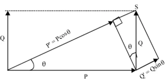
Modified triangle method is an alternative strategy for reactive power cost allocation.

According to Fig. 1 we can write:

2

P′ =P cos( )θ =Scos ( )θ (4)

2

Q′ =Q sin( )θ =Ssin ( )θ (5) Using (4) and (5) we have:

Fig. 1: Modified triangle method for reactive power cost allocation

P Q S

Cost(P ) Cost(Q ) Cost(S)

′+ ′=

′ + ′ = (6)

For expressing active power cost, we replace (4) in (2) as follows:

2 2 2

Cost(P ) Cost(P cos( ))

a b cos( )P ccos ( )P a b P c P

′ = θ

′ ′

= + θ + θ = + + (7)

Using (2) and (5) the new frame of reactive power pricing can be written as given below:

2 2

2 2 2

P

Cost(Q ) Cost(Ssin ( )) Cost( sin ( )) cos( )

a bsin( )Q csin ( )Q a b Q c Q

′ = θ = θ

θ

′′ ′′

= + θ + θ = + +

(8)

It is assumed that the reactive compensators are owned by private investors and installed at some selected buses. The charge for using capacitors is assumed proportional to the amount of the reactive power output purchased and can be expressed as:

Cj Cj j Cj

C (Q )=r Q (8)

where, rj and QCj are the reactive cost and amount

purchased, respectively, at location j. The production cost of the capacitor is assumed as its capital investment return, which can be expressed as its depreciation rate. For example, if the investment cost of a capacitor is $11600/MVA and their average working rate and life span are 2/3 and 15 years, respectively, the cost or depreciation rate of the capacitor can be calculated by:

j

investment cos t r

operating hours

$11600 $0.1324

15 365 24 2 / 3 MVAh

=

= =

× × ×

(8)

capacitors are the control variables. The equality and inequality constraints include the load flow equations, active and reactive power output of generators, reactive power output of capacitors and the bus voltage limits at the normal operating condition, as shown below:

Load flow equations:

Gi Di i j ij ij j i

Gi Di i j ij ij j i

P P V V Y cos( ) 0

Q Q V V Y sin( ) 0

− − θ + δ − δ =

− − θ + δ − δ =

∑

∑

ɺ ɺ

ɺ ɺ (9)

Active and reactive power generation limits:

Gi,min Gi Gi,max

Gi,min Gi Gi,max

P P P

Q Q Q

≤ ≤

≤ ≤ (10)

Capacitor reactive power generation limits:

Cj Cj,max

0≤Q ≤Q (11)

Transmission line limit:

ij ij,max ij i j ij

2

ij j i i ij ij

P P , P V V Y

cos( ) V Y cos

≤ =

θ + δ − δ − θ

ɺ ɺ

ɺ (12)

Bus voltage limits:

i,min i i, max

V ≤ V ≤V (13)

Where:

PDi and QDi = The specified active and reactive

demand at ith load bus, respectively

ij ij

Y∠θ = The element of the admittance

matrix

i i i

Vɺ = ∠δV = The bus voltage at ith bus

PGi,min and PGi,max = The lower and upper limits of

active power generation at ith generator, respectively

QGi,min and QGi,max = The lower and upper limits of

reactive power generation at ith generator, respectively

QCj,max = The upper limits of reactive power

output of the capacitor

Vi,min and Vi,max = The lower and upper limits of

voltage at ith bus, respectively The general-purpose optimization problem can be expressed as:

x

i eq

i ueq

min f (x)

h (X) 0 i 1.2.3....N

g (X) 0 i 1.2.3....N

= =

> =

(14)

The corresponding Lagrange function of the problem is formed as:

p m

i i p j j

i 1 j 1

L(X, ) f (X) g (X) +h (x)

= =

λ = +

∑

∑

where, λ_{i is the Lagrange multiplier for the i}th constraint.

Based on the above mathematical model the corresponding Lagrangian function of this optimization problem takes the form of (16).

According to microeconomics, the marginal prices for active power and reactive power at ith bus are λ_{pi and} λ_{qi respectively and will be taken as the corresponding} spot prices in the electricity markets[15]:

(

)

(

)

gpi Gi gqi Gi cj Cj

i G j C

pi Gi Di i j ij ij j i

i N

qi Gi Di i j ij ij j i

i N

pi,max Gi,min Gi pi,max Gi Gi,max

i G i G

cj,min Cj,min j C

L C (P ) C (Q ) C (C )

P P V V Y cos( )

Q Q V V Y sin( )

P P P P

Q

∈ ∈

∈

∈

∈ ∈

∈

 

=  + +

 

− λ  − − θ + δ − δ 

 

 

− λ  − − θ + δ − δ 

 

+ µ − + µ −

+ µ −

∑

∑

∑

∑

∑

∑

∑

∑

∑

ɺ ɺ ɺ ɺ

(

)

(

)

(

)

(

)

(

)

(

)

Cj cj, max cj cj,max

j c

2 2 2

si Gi Gi Gi,max ij ij ij, max

i G i N j N

j i

i,min i,min i i,max i i,max

i N i N

Q Q Q

P Q S P P

V V V V

∈

∈ ∈ ∈

≠

∈ ∈

+ µ −

+ µ + − + η −

+ ν − + ν −

∑

∑

∑∑

∑

∑

(16)

ANTCOLONYALGORITHM

that such capabilities are essentially due to what is called pheromone trails, which ants use to communicate information among individuals regarding path and to decide where to go. During their trips a chemical trail (pheromone) is left on the ground. The pheromone guides other ants towards the target point. Furthermore, the pheromone evaporates over time (i.e., it loses quantity if other ants lay down no more pheromone). If many ants choose a certain path and lay down pheromones, the quantity of the trail increases and thus this trail attracts more and more ants[17-19]. Each ant probabilistically prefers to follow a direction rich in pheromone rather than a poorer one.

The basic ACO method was inspired by the behavior of real ant colonies in which a set of artificial ants cooperate in solving a problem by exchanging information via pheromone deposited on a graph. The basic ACO is often to deal with the combinatorial optimization problems. The Generalized Ant Colony Optimization (GACO) can be used to solve the continuous or discontinuous, nonconvex, nonlinear constrained optimization problems. The characteristics GACO are positive feedback, distributed computation and the use of constructive greedy heuristic. The proposed GACO algorithm has the following feature.

• The points in feasible region are regard as ants. After some iteration, the ants will centralize at the optimum points, one or several. There’re two choices for an ant in each iteration: moving to other ants’ point or searching in neighborhood

• The iteration would be guided by changing the distribution of intensity of pheromone in feasible region

• The Sequential Quadratic Programming (SQP) is used as neighborhood-searching algorithm to improve the precision of convergence

• The roulette wheel selection and disturbance are used to prevent the sub-optimization in GACO The convergence property of GACO is studied based on the fixed-point theorem on a complete metric space, presents several sufficient conditions for convergence.

The procedure of a GACO method can be described as follows.

Step 1: Initialization.

Initial population: An initial population of ant colony individuals Xi (i = 1,2,…,N) is selected randomly from

the feasible region S. Typically, the distribution of

initial trials is uniform. The initial ant colony can be written as:

0 T

1 2 N i

C =(X , X ,..., X ) for X∈S

Intensity matrix: At initialization phase, the elements of trail intensity matrix (τN×N) are set to a constant

level: τij = τ0, τ0>0.

Number of ants: Let b(i) (i = 1,2,...,N) be the number of ants in point i and at the beginning b(i) = l.

Ant’s visibility: Ant’s visibility can be defined as:

0 ak / T 1

D(k) 2(1 )D

1 e

= −

+ (17)

where, K is the cycles counter and D0 is the upper limit

of ant’s visibility. With the running of GACO, the visibility D(K) decreases and the exactitude of search increases gradually. If X_i−X_j ≤D(k ) then the ants can transfer from point i to point j.

Where . is a kind of norm, which is defined as:

i1 i n 1 2 n

X =Max x _{< <} X=[x , x ,..., x ]

Step 2: For the ants on the point i (i = l,2,... N), b(i)>1, the neighborhood search for transition is defined as:

}

{

i j i j

A = X X −X ≤D(k)

If Ai≠ Φ go to step 3, else go to step 4. Here Φ is

empty set.

Step 3: Let m be the quantity of elements in the set Ai,

we set:

j i

ij i j j i

ii ak / t ij

X A

F(X ) F(X ) X A

1 2

( 1)

m 1 e− _∈

Φ = − ∀ ∈

Φ = − Φ

+

∑

(18)

where, F(X) is objective function. Transition probability is defined as:

1 2

j i

1 2 1 2

j i j i

ii ij

X A

0

ii ij ij ij

X A X A

1

( ) ( ( ))

m P

1

( ) ( ( )) ( ) ( )

m

γ γ

∈

γ γ γ γ

∈ ∈

Φ τ

=

Φ τ + Φ τ

∑

∑

∑

1 2

1 2 1 2

ij ij

ij

ii ij ij ij

X A X A

( ) ( ) P

1

( ) ( ( )) ( ) ( )

m

γ γ

γ γ γ γ

∈ ∈

Φ τ

=

where, γ1 and γ2 are parameters that control the relative

importance of trail versus visibility. P0 is the probability

of neighborhood search. We note that with the decrease of F(Xj) the τij and Pij increase. By (19) and (20) we

see:

j i

ij 0

X A

P P 1

∈ + =

∑

The roulette wheel is used for stochastic selection. If the selection result is a Pij carry out the update rule l. Update rule 1: Moving an ant from point i to point j.

b(i) = b(i)-l, b(j) = b(j)+l, ∆τij = Pij, Xi← Xj and go

to step 5.

If the selection result is P0, carry out the update

rule 2.

Update rule 2: Carrying out search by Sequential Quadratic Programming (SQP) algorithm in the neighborhood of Xi. The neighborhood defined by:

{

}

i

X i

S = Y X −Y <α.D(K)

where, α is a positive parameter and α∈(0,1). Let the result of neighborhood search be Y, then Xi← Y and:

(

)

j i

1 2 1 2

j i j i

i ij

X A

ij

ii ij ij ij

X A X A

1

F(X ) F(Y) ( ( ))

M 1

( ) ( ( )) ( ) ( )

m

γ γ

∈

γ γ γ γ

∈ ∈

− τ

∆τ =

Φ τ + Φ τ

∑

∑

∑

Go to step 5.

Step 4: Searching in neighborhood quadratic programming (SQP) algorithm. Let the result be Y, carry out the update rule 3.

Update rule 3: Xi← Y, ∆τij = r, where r is a positive

constant.

Step 5: Updating the trail intensity matrix according to the following formula:

ij(K 1) ij(k) ij i j, Xj Ai

τ + = ρτ + ∆τ ∀ ≠ ∈ (23)

where, ρ is a coefficient such that (1-ρ) represents the evaporation of trail between time K and K+1.

Step 6: After iteration all ants have complete one move, calculate the results for every Xi∈Ck. Here Ck is the ant colony in K iterations:

• If dissatisfying the convergence condition, cancel the result from step 2-4 and go to step 2

• If the results are not changed after NI iterations, disturb the ant colony by increasing the visibility and neighborhood of search. Here NI is a coefficient

• If K< T, K = K+ 1 then go to step 2, else print best result and stop

TESTSYSTEMANDSIMULATION

RESULTS

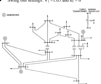
In this research IEEE 14-bus test system is used to test the proposed measurement placement algorithm. A schematic of this test system is shown in Fig. 2 and its total data are provided from[15]. There are three generators on buses 1, 2 and 9 respectively. The nominal apparent power output of each generator is I25 MVA. The lower and upper limits of power output are 20 MW and 125 MW. The active power production cost of each generator is:

2

gpi Gi Gi Gi

C (P )=75 750P+ +420P ($/hr)

All the parameters stated here are in per unit on a 100 MVA base. There are capacitors installed on bus 5 with the total capacity of 50 MVA. We assume the reactive power output can be adjusted continuously.

The other system operation limits are:

• Transmission limit: Pij ≤1.8

• Voltage limit: 0.95≤ Vi ≤1.05

• Swing bus settings: V1 =1.05 and δ1 = 0

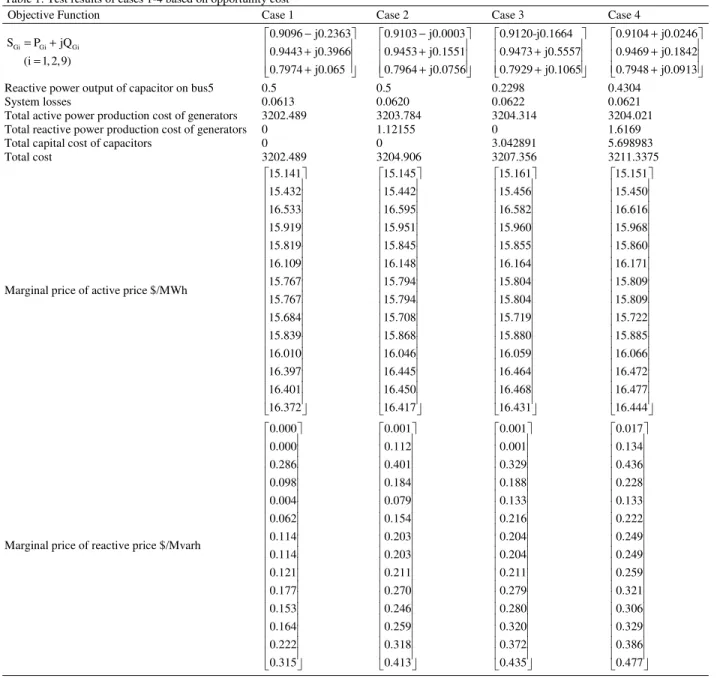
Table 1: Test results of cases 1-4 based on opportunity cost

Objective Function Case 1 Case 2 Case 3 Case 4

Gi Gi Gi

S P jQ

(i 1, 2, 9)

= + = 0.9096 j0.2363 0.9443 j0.3966 0.7974 j0.065 −     +    ₊    0.9103 j0.0003 0.9453 j0.1551 0.7964 j0.0756 −     +    ₊    0.9120-j0.1664 0.9473 j0.5557 0.7929 j0.1065     +    ₊    0.9104 j0.0246 0.9469 j0.1842 0.7948 j0.0913 +     +    ₊   

Reactive power output of capacitor on bus5 0.5 0.5 0.2298 0.4304

System losses 0.0613 0.0620 0.0622 0.0621

Total active power production cost of generators 3202.489 3203.784 3204.314 3204.021

Total reactive power production cost of generators 0 1.12155 0 1.6169

Total capital cost of capacitors 0 0 3.042891 5.698983

Total cost 3202.489 3204.906 3207.356 3211.3375

Marginal price of active price $/MWh

15.141 15.432 16.533 15.919 15.819 16.109 15.767 15.767 15.684 15.839 16.010 16.397 16.401 16.372                                             15.145 15.442 16.595 15.951 15.845 16.148 15.794 15.794 15.708 15.868 16.046 16.445 16.450 16.417                                             15.161 15.456 16.582 15.960 15.855 16.164 15.804 15.804 15.719 15.880 16.059 16.464 16.468 16.431                                             15.151 15.450 16.616 15.968 15.860 16.171 15.809 15.809 15.722 15.885 16.066 16.472 16.477 16.444                                            

Marginal price of reactive price $/Mvarh

0.000 0.000 0.286 0.098 0.004 0.062 0.114 0.114 0.121 0.177 0.153 0.164 0.222 0.315                                             0.001 0.112 0.401 0.184 0.079 0.154 0.203 0.203 0.211 0.270 0.246 0.259 0.318 0.413                                             0.001 0.001 0.329 0.188 0.133 0.216 0.204 0.204 0.211 0.279 0.280 0.320 0.372 0.435                                             0.017 0.134 0.436 0.228 0.133 0.222 0.249 0.249 0.259 0.321 0.306 0.329 0.386 0.477                                            

In order to study the impacts of various factors on the marginal price of reactive power, seven cases are studied:

• The objective function has only the first item of (l)

• The objective function has only the first two items with capacitor cost neglected

• The objective function has only the first and the third items with reactive power production cost of generators neglected

• The objective function has all the three items as described in (1)

The computer test results for cases 1 to 4 based on opportunity cost and modified triangle method for reactive power cost allocation are listed in Table 1 and 2, respectively. The four cases are used to study the impacts of OPF objective functions on reactive power marginal price (RPMP).

According to Table 1 and 2, the following results are obtained:

Table 2: Test results of cases 1-4 based on modified triangle method

Objective Function Case 1 Case 2 Case 3 Case 4

Gi Gi Gi

S P jQ

(i 1, 2, 9)

= + = 1.014 j0.165 0.8611 j0.7294 0.7811 j0.173 −     +    ₊    0.9006 j0.025 0.954 j0.11869 0.7971 j0.0683 −     +    ₊    1.014 j0.165 0.8611 j0.7294 0.7811 j0.173 −     +    ₊    0.9002 j0.0154 0.9566 j0.1965 0.795 j0.089 +     +    ₊   

Reactive power output of capacitor on bus 5 0 0.5 0 0.4289

System losses 0.0662 0.0617 0.662 0.0618

Total active power production cost of generators 2886.736 3171.453 2886.736 3166.595 Total reactive power production cost of generators 0 257.392 0 262.967

Total capital cost of capacitors 0 0 0 5.67859

Total cost 3202.489 3428.846 2886.736 3435.241

Marginal price of active price $/MWh

16.1120 14.0782 14.3715 14.7567 14.9852 15.0024 14.6970 14.6970 14.6624 14.7433 14.8777 15.2723 15.4199 15.2009                                             15.0621 15.3523 16.4938 15.8573 15.7530 16.0539 15.7009 15.7009 15.6155 15.7749 15.9522 16.3486 16.3535 16.3211                                             16.1120 14.0782 14.3715 14.7567 14.9852 15.0024 14.6970 14.6970 14.6624 14.7433 14.8777 15.2723 15.4199 15.2009                                             15.0606 15.3555 16.5134 15.8729 15.7655 16.0763 15.7143 15.7144 15.6277 15.7903 15.9716 16.3783 16.3872 16.3701                                            

Marginal price of reactive price $/Mvarh

2.5378 4.8973 3.9693 3.1288 2.6011 2.1705 2.8925 2.8925 2.7661 2.6321 2.3893 1.9138 1.7177 2.2207                                             0.0014 0.0998 0.3888 0.1780 0.0739 0.1447 0.1982 0.1982 0.2072 0.2647 0.2393 0.2492 0.3084 0.4060                                             2.5378 4.8973 3.9693 3.1288 2.6011 2.1705 2.8925 2.8925 2.7661 2.6321 2.3893 1.9138 1.7177 2.2207                                             0.0009 0.1204 0.4272 0.2284 0.1324 0.2488 0.2703 0.2703 0.2911 0.3525 0.3350 0.3608 0.4229 0.5491                                            

• For each test case, active power marginal prices at various buses are in the same order while the RPMP fluctuates significantly from bus to bus. Generally the active power marginal price is much higher than the RPMP at a certain bus. In our case it is about 100 times as much as RPMP under normal conditions

• The total reactive power production cost changes apparently along with the objective function change. Although the cost is small, it can accumulate into a large amount

• When the capacitor cost and/or the reactive power generation cost is neglected, the corresponding reactive power source bus(es) will have zero or

• When the modified triangular method is used for reactive power pricing, the corresponding RPMP at all bus increases noticeably

• The proposed method based on the ant colony algorithms and advanced sequential quadratic programming capable to find global optimum solution for the OPF problem

CONCLUSIONS

In this study the reactive power marginal price is studied in detail. Both active and reactive power production costs of generators and capital cost of capacitors are considered in the objective function of OPF problem. Then a new method based on the ant colony algorithms and advanced sequential quadratic programming is employed to solve the OPF problem.

The IEEE 14-bus system was used to test the validity of the methodology, considering four objective functions. Test results may confirm that participation of the generators in the reactive power market is important for the participants of a competitive electric market.

It has been observed that the reactive power marginal price is typically less than 3% of the corresponding active power marginal price.

Based on this study the major conclusions of this work are:

• The reactive power production cost and the capital investment of capacitors should be considered in reactive power spot pricing for their noticeable impacts on reactive power marginal price

• Reactive power marginal cost can serve as a system index related to the urgency of the reactive power supply and system voltage support and an incentive to improve load power factor and reduce reactive power demand

• When the modified triangular method is used for reactive power pricing, the corresponding RPMP at all bus increases noticeably

REFRENCES

1. Loi Lei Lai, 2001. Power System Restructuring and Deregulation. John Wiley, http://www.wiley.com. 2. Berg, S.V., J. Adams and B. Niekum, 1983. Power

factors and the efficient pricing and production of reactive power. Energy J., 4: 93-102.

3. Schweppe F.C., M.C. Caramanis, R.D. Tabors and R.E. Bohn, 2000. Spot Pricing of Electricity. Kluwer, MA, USA.

4. Baughman, M.L. and S.N. Siddiqi, 1991. Real-time pricing of reactive power: Theory and case study results. IEEE Trans. Power Syst., 6: 23-29. DOI: 10.1109/59.131043.

5. El-Keib, A.A. and X. Ma, 1997. Calculating short-run marginal costs of active and reactive power production. IEEE Trans. Power Syst., 12: 559-565. DOI: 10.1109/59.589604.

6. Chattopadhyay, D., K. Bhattacharya and J. Parikh, 1995. Optimal reactive power planning and its spot-pricing: An integrated approach. IEEE Trans. Power Syst., 10: 2014-2020. DOI: 10.1109/59.476070.

7. Li, Y.Z. and A.K. David, 1994. Wheeling rates of reactive power flow under marginal cost pricing. IEEE Trans. Power Syst., 9: 1263-1269. DOI: 10.1109/59.336141.

8. Hao, S. and A. Papalexopoulos, 1997. Reactive power pricing and management. IEEE Trans. Power Syst., 12: 95-104. DOI: 10.1109/59.574928. 9. Miller, T.J., 1982. Reactive power control in

electric systems. Wiley, NJ, USA.

10. Dandachi, N.H., M.J. Rawlins,, 0. Alsac, M. Paris and, B. Stott, 1996. OPF for reactive pricing studies on the NGC system. IEEE Trans. Power Syst., 11: 226-232. DOI: 10.1109/59.486099. 11. Choi, J.Y., S.H. Rim and J.K. Park, 1998. Optimal

real time pricing of real and reactive powers. IEEE Trans. Power Syst., 13: 1226-1231. DOI: 10.1109/59.736234.

12. Gil, J.B., T.G. San Roman, J.A. Rios and P.S. Martin, 2000. Reactive power pricing: A conceptual framework for remuneration and charging procedures. IEEE Trans. Power Syst., 15: 483-489. DOI: 10.1109/59.867129.

13. Lamont, J.W. and J. Fu, 1999. Cost analysis of reactive power support. IEEE Trans. Power Syst., 14: 890-896. DOI: 10.1109/59.780900.

14. Zhao, Y., M.R. Irving and Y. Song, 2005. A cost allocation and pricing method for reactive power service in the new deregulated electricity market environment. In: IEEE/PES Transmission and Distribution Conference Asia and Pacific, 1: 6, DOI: 10.1109/TDC.2005.1547186.

15. Chung, C.Y., T.S. Chung, C.W. Yu and X.J. Lin, 2004. Cost-based reactive power pricing with voltage security consideration in restructured power systems. Electric Power systems Research, 70: 85-91, DOI 10.1016/j.epsr.2003.11.002. 16. Dorigo, M., 1992. Optimization, learning and

natural algorithms. Ph.D Thesis, Politecnico de Milano, Italy.

17. Dorigo, M., V. Maniezzo and A. Colorni, 1996. Ant system: optimization by a colony of cooperating agents. IEEE Trans. Syst. Man Cybernet., 26: 29-41. DOI: 10.1109/3477.484436. 18. Dorigo, M., G.D.Caro and L.M Gambardella,

1999. Ant’s algorithm for discrete optimization. Artificial Life, 5: 137-172.