www.atmos-chem-phys.net/17/385/2017/ doi:10.5194/acp-17-385-2017
© Author(s) 2017. CC Attribution 3.0 License.
Direct oceanic emissions unlikely to account for the missing source
of atmospheric carbonyl sulfide
Sinikka T. Lennartz1, Christa A. Marandino1, Marc von Hobe2, Pau Cortes3, Birgit Quack1, Rafel Simo3,
Dennis Booge1, Andrea Pozzer4, Tobias Steinhoff1, Damian L. Arevalo-Martinez1, Corinna Kloss2, Astrid Bracher5,6, Rüdiger Röttgers7, Elliot Atlas8, and Kirstin Krüger9
1GEOMAR Helmholtz Centre for Ocean Research Kiel, Düsternbrooker Weg 20, 24105 Kiel, Germany 2Forschungszentrum Jülich GmbH, Institute of Energy and Climate Research (IEK-7), Wilhelm-Johnen-Strasse,
52425 Jülich, Germany
3Institut de Ciencies del Mar, CSIC, Pg. Maritim de la Barceloneta, 37-49, 08003 Barcelona, Catalonia, Spain 4Max Planck Institute for Chemistry, Hahn-Meitner-Weg 1, 55128 Mainz, Germany
5Alfred Wegener Institute Helmholtz Centre for Polar and Marine Research, Bussestrasse 24, 27570 Bremerhaven, Germany 6Institute of Environmental Physics, University of Bremen, 28334 Bremen, Germany
7Helmholtz-Zentrum Geesthacht, 21502 Geesthacht, Germany
8Rosenstiel School of Marine and Atmospheric Science, Miami, FL 33149, USA 9University of Oslo, Department of Geosciences, 0315 Oslo, Norway
Correspondence to:Sinikka T. Lennartz ([email protected])
Received: 29 August 2016 – Published in Atmos. Chem. Phys. Discuss.: 12 September 2016 Revised: 22 November 2016 – Accepted: 6 December 2016 – Published: 10 January 2017
Abstract. The climate active trace-gas carbonyl sulfide (OCS) is the most abundant sulfur gas in the atmosphere. A missing source in its atmospheric budget is currently sug-gested, resulting from an upward revision of the vegetation sink. Tropical oceanic emissions have been proposed to close the resulting gap in the atmospheric budget. We present a bottom-up approach including (i) new observations of OCS in surface waters of the tropical Atlantic, Pacific and Indian oceans and (ii) a further improved global box model to show that direct OCS emissions are unlikely to account for the missing source. The box model suggests an undersaturation of the surface water with respect to OCS integrated over the entire tropical ocean area and, further, global annual direct emissions of OCS well below that suggested by top-down es-timates. In addition, we discuss the potential of indirect emis-sion from CS2and dimethylsulfide (DMS) to account for the
gap in the atmospheric budget. This bottom-up estimate of oceanic emissions has implications for using OCS as a proxy for global terrestrial CO2uptake, which is currently impeded
by the inadequate quantification of atmospheric OCS sources and sinks.
1 Introduction
Carbonyl sulfide (OCS) is the most abundant reduced sul-fur compound in the atmosphere. It enters the atmosphere ei-ther by direct emissions, e.g., from oceans, wetlands, anoxic soils or anthropogenic emissions, or indirectly via oxidation of the short-lived precursor gases dimethylsulfide (DMS) and carbon disulfide (CS2) (Chin and Davis, 1993; Watts, 2000;
Kettle, 2002). Both precursor gases are naturally produced in the oceans, and CS2has an additional anthropogenic source
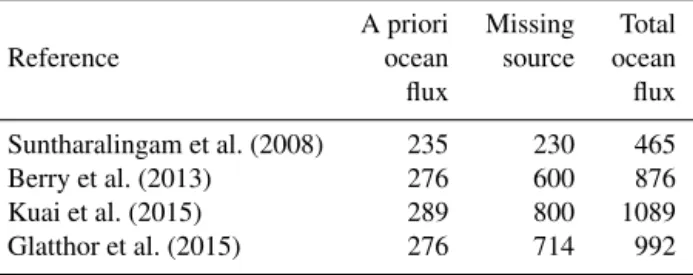
Table 1. Missing source estimates derived from top-down ap-proaches: the listed studies used an increased vegetation sink and an a priori direct and indirect ocean flux to estimate the magnitude of the missing source. Assigning the missing source to oceanic emis-sions results in the total ocean flux listed here. Fluxes are given in Gg S per year.
A priori Missing Total
Reference ocean source ocean
flux flux
Suntharalingam et al. (2008) 235 230 465 Berry et al. (2013) 276 600 876 Kuai et al. (2015) 289 800 1089 Glatthor et al. (2015) 276 714 992
Accurate accounts of sources and sinks of atmospheric OCS are crucial for two reasons.
– First, OCS is climate-relevant because it influences the radiative budget of the Earth as a greenhouse gas and by contributing significant amounts of sulfur to the strato-spheric aerosol layer (Crutzen, 1976; Brühl et al., 2012; Notholt et al., 2003; Turco et al., 1980) that exerts a cooling effect (Turco et al., 1980; Kremser et al., 2016). The two opposite effects are currently in balance (Brühl et al., 2012), but future changes in atmospheric circula-tion, as well as the magnitude and distribution of OCS sources and sinks, could change that. Hence, a better understanding of the tropospheric budget is needed to predict the effect of OCS in future climate scenarios (Kremser et al., 2016).
– Second, OCS has recently been suggested as a promis-ing tool to constrain terrestrial CO2 uptake, i.e., gross
primary production (GPP), as it is taken up by plants in a similar way as CO2 (Asaf et al., 2013). GPP, a
ma-jor global CO2flux, can only be inferred from indirect
methods, because the uptake of CO2occurs along with
a concurrent release by respiration. Unlike CO2, OCS is
irreversibly degraded within the leaf. GPP can thus be estimated based on the uptake ratio of OCS and CO2,
from the leaf to regional scale (Asaf et al., 2013) or even global scale (Beer et al., 2010), under the condition that other sources are negligible or well quantified. The magnitude of terrestrial biogeochemical feedbacks on climate has been suggested to be similar to that of phys-ical feedbacks (Arneth et al., 2010). In order to reduce existing uncertainties, it is thus crucial to better con-strain single processes in the carbon cycle, especially GPP.
Nonetheless, current figures for tropospheric OCS sources and sinks carry large uncertainties (Kremser et al., 2016). While the budget has been previously considered closed (Kettle, 2002), a recent upward revision of the vegetation
sink (Sandoval-Soto et al., 2005; Suntharalingam et al., 2008; Berry et al., 2013) led to a gap, i.e., a missing source in the at-mospheric budget of 230–800 Gg S per year (Suntharalingam et al., 2008; Berry et al., 2013; Kuai et al., 2015; Glatthor et al., 2015) (Table 1), with the most recent estimates at the higher end of the range. This revision of vegetation uptake was suggested to (i) take into account the different deposi-tion velocities of CO2and OCS within the leaf and base it on
GPP instead of net primary production (Sandoval-Soto et al., 2005) as well as (ii) to better reproduce observed seasonality of OCS mixing ratios in several atmospheric models (Berry et al., 2013; Kuai et al., 2015; Glatthor et al., 2015). Based on independent top-down approaches using MIPAS (Glatthor et al., 2015) and TES (Kuai et al., 2015) satellite observa-tions, FTIR measurements (Wang et al., 2016), and NOAA ground-based time series stations and the HIPPO aircraft campaign (Berry et al., 2013; Kuai et al., 2015), the missing source of OCS was suggested to originate from the (tropi-cal) ocean, most likely from the region of the Pacific warm pool. Other potential sources such as advection of air masses from Asia have been discussed (Glatthor et al., 2015) but not tested. If the ocean was to account for the missing source, the total top-down oceanic source strength would then be the a priori oceanic flux plus the missing source estimate of each inverse model simulation (Table 1). This addition would im-ply a 200–380 % increase in the a priori estimated oceanic source. If oceanic direct and indirect emissions were to ac-count for the total missing source, an ocean source strength of 465–1089 Gg S yr−1would be required (Table 1).
OCS and its atmospheric precursors are naturally pro-duced in the ocean. In the surface open ocean, OCS is present in the lower picomolar range, and has been measured on nu-merous cruises in the Atlantic (Ulshöfer et al., 1995; Flöck and Andreae, 1996; Ulshöfer and Andreae, 1998; von Hobe et al., 1999), including three latitudinal transects (Kettle et al., 2001; Xu et al., 2001), the Indian Ocean (Mihalopou-los et al., 1992), the Pacific Ocean (Weiss et al., 1995a) and the Southern Ocean (Staubes and Georgii, 1993). Measure-ments in tropical latitudes, where the missing source is as-sumed to be located, have previously been performed in the Indian Ocean (Mihalopoulos et al., 1992) and during the At-lantic transects (Kettle et al., 2001; Xu et al., 2001). OCS is produced photochemically from chromophoric dissolved organic matter (CDOM) (Andreae and Ferek, 2002; Ferek and Andreae, 1984) and by a not fully understood light-independent production that has been suggested to be linked to radical formation (Flöck et al., 1997; Pos et al., 1998). Dissolved OCS is efficiently hydrolyzed to CO2and H2S at
a rate depending on pH and temperature (Elliott et al., 1989). CS2 has been measured in the Pacific and Atlantic oceans
in a range of 7.2–27.5 pmol L−1(Xie et al., 1998) and dur-ing two Atlantic transects (summer and winter) in a range of 4–40 pmol L−1 (Xu, 2001). It is produced photochemically
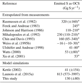
Table 2.Global oceanic emission estimates of OCS: direct ocean emission estimates of OCS from bottom-up approaches. Uncertain-ties are given in parentheses as in the original paper either as range or±standard deviation.
Reference Emitted S as OCS
(Gg S yr−1)
Extrapolated from measurements
Rasmussen et al. (1982) 320 (±160)∗ Ferek and Andreae (1983) 245∗ Johnson and Harrison (1986) 110–210∗ Mihalopoulos et al. (1992) 230 (110–210)∗ Chin and Davis (1993) 160 (85–340)∗ Weiss et al. (1995b) −16 (−10–30)∗ Ulshöfer and Andreae (1998) 41–80∗
Watts (2000) 53 (±80)∗
Xu et al. (2001) 53∗
Model simulations
Kettle (2002) 41 (±154)
Launois et al. (2015a) 813 (573–3997)
This study 130 (±80)
∗Units deviate from original paper, converted to Gg S for comparison.
been identified (Xie et al., 1998). DMS is present in the lower nanomolar range in the surface ocean and has been exten-sively studied in several campaigns, summarized in a clima-tology by Lana et al. (2011). DMS is biogenically produced and consumed in the surface ocean, as well as photo-oxidized and ventilated by air–sea exchange (Stefels et al., 2007).
Available bottom-up estimates of the global oceanic OCS fluxes from shipboard observations range from −16 to 320 Gg S yr−1(Table 2). However, the highest estimates were biased, because mainly summertime and daytime observa-tions of water concentraobserva-tions were considered. With the dis-covery of the seasonal oceanic sink of OCS during winter-time (Ulshöfer et al., 1995) and a pronounced diel cycle (Ferek and Andreae, 1984), direct oceanic emissions were corrected downwards.
Only recently, OCS emissions have been estimated with the biogeochemical ocean model NEMO-PISCES (Launois et al., 2015a) at a magnitude of 813 Gg S yr−1, sufficient to
account for the missing source. This oceanic emission in-ventory had been used to constrain GPP based on OCS on a global scale (Launois et al., 2015b). However, the oceanic OCS photoproduction in the ocean model included a param-eterization for OCS photoproduction derived from an exper-iment in the North Sea (Uher and Andreae, 1997b), which might not be representative for the global ocean, as indicated by photoproduction constants that were an order of magni-tude lower in the Atlantic ocean compared to the German Bight (Uher and Andreae, 1997a).
Here, we present new observations in all three tropical ocean basins, two of them measured with unprecedented
pre-cision and time resolution. Direct fluxes were inferred from continuous OCS measurements in the tropical Pacific and Indian oceans, covering a range of regimes with respect to CDOM content, ultraviolet (UV) radiation and sea surface temperature (SST). These observations are used to further constrain and validate a biogeochemical box model which had previously been shown to reproduce OCS concentra-tion in the Atlantic Ocean reasonably well (von Hobe et al., 2001). The box model is now updated from its previous global application (Kettle, 2002) by adding and further de-veloping the most recent process parameterizations to esti-mate the global source strength of direct OCS emissions. The emission estimate is further complemented by discussing the potential of indirect OCS emissions, i.e., the emissions of short-lived precursor gases CS2and DMS, to account for the
gap in the budget.
2 Methods 2.1 Study sites
Several cruises were conducted to measure the trace gases OCS (OASIS, TransPEGASO, ASTRA-OMZ) and CS2
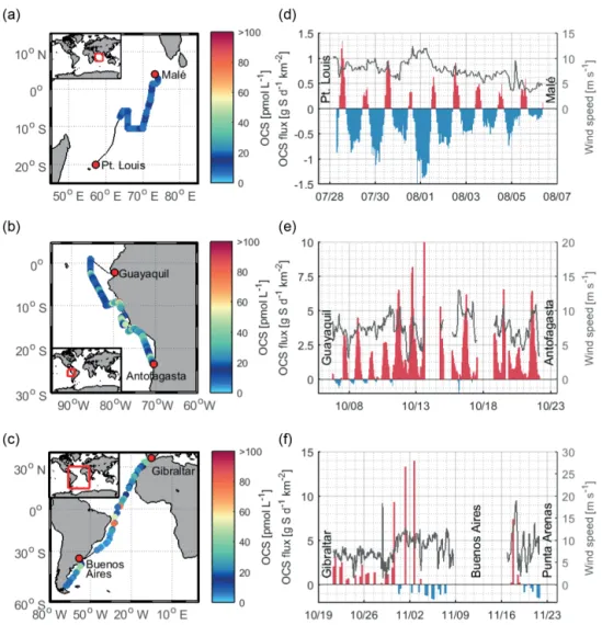
(TransPEGASO, ASTRA-OMZ). Cruise tracks are depicted in Fig. 1. The OASIS cruise onboard RVSONNE Ito the In-dian Ocean started from Port Louis, Mauritius, to Malé, Mal-dives, in July and August 2014, where mainly oligotrophic waters were encountered. TransPEGASO was an Atlantic transect starting in Gibraltar and leading to Buenos Aires, Argentina, and Punta Arenas, Chile. It took place in October and November 2014 and covered a variety of biogeochemi-cal regimes. ASTRA-OMZ onboard RVSONNE IIstarted in Guayaquil, Ecuador, and ended in Antofagasta, Chile, in Oc-tober 2015. Although 2015 was an El Niño year, upwelling together with high biological production was still encoun-tered during the cruise (Stramma et al., 2016).
2.2 Measurement setup for trace gases
OCS was measured during two cruises onboard the RV
SONNE I (OASIS) and SONNE II (ASTRA-OMZ) with a continuous underway system similar to the one described in Arévalo-Marténez et al. (2013), at a measurement fre-quency of 1 Hz. The system consisted of a Weiss-type equilibrator, through which seawater is pumped from ap-proximately 5 m below the surface with a flow of 3– 4 L min−1. The air from the equilibrator headspace was
Figure 1.Observed OCS water concentrations and calculated emissions: observations of OCS concentrations in the surface ocean during the three cruises (a)OASIS,(b)ASTRA-OMZ, and(c)TransPEGASO as well as the corresponding emissions calculated based on the concentration gradient between water and marine boundary layer(d–f). Outgassing is indicated in red bars; oceanic uptake in blue bars. The grey line shows wind speed measured onboard the vessels. Flux data are shown with different scales on theyaxes. Data gaps occurred during stays in port and territorial waters or during instrument tests.
2 min, achieving a precision of 15 ppt. OCS mixing ratios in the marine boundary layer (MBL) were determined by pump-ing outside air ca. 50 m from the ship’s deck to the OCS an-alyzer (KNF Neuberger pump). A measurement cycle con-sisted of 50 min water sampling and 10 min air sampling, where the first 3 min after switching until stabilization of the signal were discarded.
Before and after the cruise the analyzer was calibrated over a range of concentrations using permeation devices. Both calibrations were consistent. However, during calibration the output of the internal spectral retrieval differed significantly from post-processing of the recorded spectra, which matched the known concentrations (this offset is not present in the commercial instruments). The calibration data were thus used to derive a correction function. After correction all data stayed within 5 % of the standards. The calibration scale of the permeation devices was 5 % below the NOAA scale. As
the OCS analyzer measured CO2simultaneously, and CO2
standards were available during the cruise, drift of the instru-ment was tested by measuring CO2standard gases before and
after the cruise and found to be less than 1 % of the signal. Special care was taken to avoid contamination, and all mate-rials used were tested for contamination before use.
During OASIS, the mirrors inside the cavity of the OCS analyzer were not completely clean, which led to a reduced signal. To correct the data, an attenuation factor was deter-mined from simultaneous CO2 measurements, because no
OCS standard was available onboard, and OASIS data were corrected accordingly.
at-tenuation corrected for OASIS) OA-ICOS data were on av-erage 5 % lower than the air canister samples, which reflects the 5 % difference between the calibration at Forschungszen-trum Jülich and the NOAA scale.
During ASTRA-OMZ, CS2 was directly measured
on-board within 1 h of collection using a purge and trap sys-tem attached to a gas chromatograph and mass spectrome-ter (GC/MS; Agilent 7890A/Agilent 5975C; inert XL MSD with triple axis detector) running in single-ion mode. The discrete surface seawater samples (50 mL) were taken each hour to every 3 h from the same pump system as for contin-uous OCS measurements. CS2was stripped by purging with
helium (70 mL min−1) for 15 min. The gas stream was dried
using a Nafion membrane dryer (Perma Pure) and CS2was
preconcentrated in a trap cooled with liquid nitrogen. After heating the trap with hot water, CS2 was injected into the
GC/MS. Retention time for CS2 (m/z76, 78) was 4.9 min.
The analyzed data were calibrated each day using gravimet-rically prepared liquid CS2standards in ethylene glycol.
Dur-ing purgDur-ing, 500 µL gaseous deuterated DMS (d3-DMS) and isoprene (d5-isoprene) were added to each sample as an inter-nal standard to account for possible sensitivity drift between calibrations.
During the TransPEGASO cruise onboard RVHesperides, surface ocean OCS and CS2were measured in discrete
sea-water samples by purge and trap and gas chromatography with mass spectrometry detection (GC-MSD). Samples were collected every day at 09:00 and 15:00 local time in glass bottles without headspace and analyzed within 1 h. Aliquots of 25 mL were withdrawn with a glass syringe and filtered through GF/F during injection into the purge and trap system (Stratum, Teledyne Tekmar). The water was heated to 30◦C and volatiles were stripped by bubbling with 40 mL min−1of
ultrapure helium for 12 min and trapped in a U-shaped VO-CARB 9 trap at room temperature. After flash thermal des-orption, volatiles were injected into an Agilent 5975T LTM GC-MSD equipped with an Agilent LTM DB-VRX column (20 m×0.18 mm OD×1 µm) maintained at 30◦C. Reten-tion times for OCS (m/z60) and CS2(m/z76) were 1.3 and
2.7 min, respectively. Peak quantification was achieved with respect to gaseous (OCS in N2) and liquid (CS2in methanol
and water) standards that were analyzed in the same way. Samples were run in duplicates. Detection limits were 1.8 pM (OCS) and 1.4 pM (CS2), and precision was typically around
5 %.
The systems are each calibrated against a standard, but they had not been directly intercompared. Still, our measure-ments are consistent with previous measuremeasure-ments using in-dependent methods as discussed in Sects. 3.2.1 and 3.3. 2.3 Calculation of air–sea exchange
FluxesF of all gases were calculated with Eq. (1):
F =kw·1C, (1)
wherekwis the gas transfer velocity in water (i.e., physical constraints on exchange) and1C the air–sea concentration gradient (i.e., the chemical constraint on exchange). The air-side transfer velocity (Liss and Slater, 1974) for OCS was calculated to be 7 orders of magnitude smaller and was there-fore neglected. The concentration gradient was determined using the temperature dependent Henry constant (De Bruyn et al., 1995) and the measurements in the surface water and MBL for OASIS and ASTRA-OMZ. During TransPEGASO, no atmospheric volume mixing ratio was measured, and a value of 500 ppt was assumed (Montzka et al., 2007). As air volume mixing ratios of OCS vary over the course of a year, we performed a sensitivity test for a scenario of 450 and 550 ppt and found mean deviations of+7.8 and−7.8 %, respectively. The transfer velocitykwwas determined using a
quadratic parameterization based on wind speed (Nightingale et al., 2000) which was directly measured onboard (10 min averages). Furthermore,kw was corrected for OCS and CS2
by scaling it with the Schmidt number calculated from the molar volume of the gases (Hayduk and Laudie, 1974). It should be noted that the choice of the parameterization for kwhas a non-negligible influence on the global emission
esti-mate. Linear, quadratic and cubic parameterizations ofkware
available, with differences increasing at high wind speeds on the order of a factor of 2 (Lennartz et al., 2015; Wanninkhof et al., 2009). Evidence suggests that the air–sea exchange of insoluble gases such as CO2, OCS and CS2 follows a
cu-bic relationship to wind speed because of bubble-mediated gas transfer (McGillis et al., 2001; Asher and Wanninkhof, 1998). However, this difference between soluble and non-soluble gases is not always consistent (Miller et al., 2009), and too few data are available for a reliable parameterization at high wind speeds above 12 m s−1, where the cubic and the
quadratic parameterizations diverge the most. For reasons of consistency, e.g., for the fitted photoproductionpfrom pre-vious studies, and the fact that most of the prepre-vious emission estimates were computed using a quadratickw
2.4 Box model of OCS concentration in the surface ocean
A box model to simulate surface concentration of OCS is further developed from the latest version from von Hobe et al. (2003, termed vH2003), where concentrations along the tracks of five Atlantic cruises have been simulated and com-pared. The vH2003 model results from successful tests and validation to observations on several cruises to the Atlantic Ocean covering all seasons (i.e., Flöck and Andreae, 1996, in January 1994; Uher and Andreae, 1997a, in April/May 1992; von Hobe et al., 1999, in June/July 1997; Kettle et al., 2001, in September/October 1998). By comparing photopro-duction rate constants of the five cruises to CDOM absorp-tion, von Hobe et al. (2003) suggest a second-order process for photoproduction with the photoproduction rate constant being dependent on the absorption of CDOM in seawater.
In our approach, we test vH2003 along the cruise track of two cruises, include a new way of determining the pho-toproduction rate constant (see below) and apply it with global climatological input (termed L2016). Kettle (2000, 2002, termed K2000) applied a similar version of vH2003 globally, which included an optimized photoproduction stant from Atlantic transect cruise data, an optimized con-stant light-independent production and a linear regression to obtain CDOM from chlorophylla. In comparison to K2000, we use (i) a new way of determining the photoproduction rate constant incorporating information from three ocean basins, (ii) the most recent parameterization of light-independent production available, and (iii) satellite observations for sea surface CDOM instead of an empirical relationship based on chlorophylla.
Launois et al. (2015a) implemented parameterizations for light-independent production, hydrolysis and air–sea ex-change similar to vH2003 in the 3-D global ocean model NEMO-PISCES. The main differences to the approach used here are the lack of accounting for mixing in L2016 (dis-cussed in Sect. 3.2.2, which will theoretically lead to higher simulated concentrations in our case) and the application of a photoproduction rate constant in our model that incorporates information from three open ocean basins in contrast to one from a study in the North Sea (Launois et al., 2015a).
In L2016, the light-independent production term of OCS was parameterized depending on SST (K) and the absorption coefficient of CDOM at 350 nm wavelength,a350(von Hobe
et al., 2001) (Eq. 2).
dCOCS
dt =a350×10 −6
×exp
55.8−16 200 SST
(2)
An overview on symbols and abbreviations used in equations in the following is provided in the Appendix. The parameter-ization for hydrolysis describes alkaline and acidic
degrada-tion of OCS by Reacdegrada-tions (R1) and (R2):
OCS+H2O→H2S+CO2, (R1)
OCS+OH−→SH−+CO2. (R2)
It was parameterized as a first-order kinetic reaction includ-ing the rate constantkhaccording to Eqs. (3)–(5):
dCOCS
dt = [OCS] ·kh, (3)
kh=exp
24.3−10 450 SST
+exp
22.8−6040 SST
· K a[H+],
(4) −log10K=3046.7
SST +3.7685+0.0035486· √
SSS, (5) wherea[H+] is the proton activity andKthe ion product of seawater (Dickinson and Riley, 1979).
Fluxes were calculated with Eq. (1) using the same pa-rameterization for kw as for the emission calculation from
measurements described above.
Photoproduction was integrated over the mixed layer depth (MLD), assuming a constant concentration of OCS and CDOM throughout the mixed layer, with the photoproduc-tion rate constantp(mol J−1),a350(m−1) and UV radiation (W m−2) (Sikorski and Zika, 1993) (Eq. 6).
dCOCS
dt =
0 Z
−MLD
pa350UVdz (6)
MLD was obtained from CTD (conductivity, temperature, depth) profiles and interpolated between these locations (Figs. S1, S2 in the Supplement). The photochemically active radiation that reaches the ocean surface was approximated by Eq. (7) (Najjar et al., 1995):
UV=2.85×10⁻⁴·I·cos2θ, (7)
with global radiationI (W m−2) and the zenith angle cosθ.
The attenuated UV light intensity directly below the surface (Sikorski and Zika, 1993) down to the respective depth of the mixed layer was calculated in 1 m steps, taking into account attenuation by CDOM and pure seawater. As a simplification in this global approach, the box model did not resolve the whole wavelength spectrum, but rather useda350and applied
a photoproduction rate constant that takes into account the integrated spectrum. A similar approach had been tested and compared to a wavelength spectrum resolving version by von Hobe et al. (2003).
Figure 2. Box model simulations compared to observations: comparison of simulated OCS water concentrations against measurements from the OASIS cruise to the Indian Ocean(a)and the eastern Pacific Ocean during the ASTRA-OMZ cruise(b). Blue indicates OCS concentrations with a least-squares fit for the photoproduction rate constantpduring daylight, fitted individually for days with homogeneous water masses (SST,a350). Black shows the simulation including thepdepending ona350, obtained from linear regression of individually fittedpwitha350(r=0.71). The time on thexaxis is local time (GMT+5 during OASIS 2014, GMT−4 during ASTRA-OMZ 2015).
a350[m-1]
0 0.05 0.1 0.15 0.2 0.25 0.3 0.35 0.4
p[pmolJ
-1]
0 500 1000 1500 2000 2500
p = 3591.3 a350+ 329.4, r = 0.7
vonHobeetal.(2003) Thisstudy:OASIS Thisstudy:ASTRA-OMZ
Linear fit
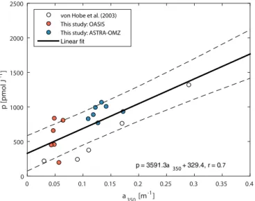
Figure 3.Dependence of photoproduction rate constantpona350
including own fits forp(resulting in blue lines in Fig. 2) and fits from a similar study (von Hobe et al., 2003). Dashed lines indicate the 95 % confidence interval.
von Hobe et al., 2001). However, the photoproduction rate constantpis not well constrained and no generally applica-ble parameterization exists. In the study of von Hobe et al. (2003), a start was made in parameterizing p in terms of CDOM absorption, and they found this to be dependent on the exact model setup used with respect to wavelength inte-gration and mixed layer treatment. To extend thep–CDOM relationship for other ocean basins, we use the two cruises OASIS and ASTRA-OMZ as case studies for parameter op-timization of the photoproduction rate constantp. The pho-toproduction constantpin the case study simulations was fit-ted individually for periods of daylight>100 W m−2(Fig. 2, blue lines) with a Levenberg–Marquardt optimization rou-tine in MatLab version 2015a (8.5.0) by minimizing resid-uals between simulated and hourly averaged measurements. Different starting values were tested to reduce the risk of the fittedpbeing a local minimum. Together with photoproduc-tion rate constants obtained by a similar optimizaphotoproduc-tion pro-cedure by von Hobe et al. (2003) (Table 2 therein, termed MLB STC), a relationship of the photoproduction constant pdependent ona350was established (Fig. 3). The resulting
a globally valid dependence. For the global box model, p was calculated in every time step based on this relationship (r=0.71, Eq. 8):
p=3591.3·a350+329.4 (8)
The scatter in Fig. 3 likely reflects the inhomogeneity of the water masses across the three oceanic basins considered, as CDOM absorbance is a valid proxy, but carries some uncer-tainty in the concentration of the actual precursor.
The model input for simulations of the cruises OASIS and ASTRA-OMZ consisted of measurements made during the respective cruise, including SST and SSS (MicroCAT SBE41) measured every minute, CDOM absorption coeffi-cient (spectrophotometrically measured ca. every 3 h with a liquid capillary cell setup) and the ship’s in situ measured meteorological data such as wind speed and global radiation averaged over 10 min (Figs. S1, S2, Tables S1, S2). Forcing data were linearly interpolated to the time step of integration of 2 min.
For the global box model, monthly global meteorological fields with a spatial resolution of 2.8◦×2.8◦were used (Ta-ble S3, Fig. S3). For globala350at the sea surface, monthly
climatological means for absorption due to gelbstoff and de-tritusa443(gelbstoff representing CDOM) from the
MODIS-Aqua satellite (all available data, 2002–2014) (NASA, 2014) were corrected to 350 nm with Eq. (9) (Fichot and Miller, 2010; Launois et al., 2015a):
a350=a443·exp(−0.02·(350−443)). (9)
SST, wind speed, and atmospheric pressure were obtained as monthly climatological means from the same period, i.e., 2002 to 2014, by ERA-Interim (Dee et al., 2011). A diel cy-cle of global radiation I was obtained by fitting the para-ble parameters aandb during time of the dayt in Eq. (10) (Fig. S4),
I = −a·t2+b, (10)
to conditions of (i)xaxis interceptions in the distance of the sunshine duration and (ii) the integral being the daily incom-ing energy by ERA-Interim (Dee et al., 2011). Monthly cli-matologies of mixed layer depths were used from the MI-MOC project (Schmidtko et al., 2013). For details of data sources please refer to Tables S1–S3 provided in the Supple-ment. The time step of the model was set to 120 min, which had been tested to result in negligible (<3 %) smoothing. 2.5 Assessing the indirect contribution of DMS with
EMAC
Model outputs from ECHAM/MESSy Atmospheric Chem-istry (EMAC) from the simulation RC1SDbase-10a of the ESCiMo project (Jöckel et al., 2016) are used to evaluate the contribution of DMS on the production of OCS. The model results were obtained with ECHAM5 version 5.3.02
and MESSy version 2.51, with a T42L90MA resolution (cor-responding to a quadratic Gaussian grid of approx. 2.8 by 2.8◦in latitude and longitude and 90 vertical hybrid pressure levels up to 0.01 hPa). The dynamics of the general circula-tion model were nudged by Newtonian relaxacircula-tion towards ERA-Interim reanalysis data. DMS emissions were calcu-lated with the AIRSEA submodel (Pozzer et al., 2006), which takes into account concentration of DMS in the atmosphere and in the ocean, following a two-layer conceptual model to calculate emissions (Liss and Slater, 1974). While atmo-spheric concentrations are estimated online by the model (with DMS oxidation), the oceanic concentrations are pre-scribed as monthly climatologies (Lana et al., 2011). It was shown that such an online calculation of emissions provides the most realistic results when compared to measurements compared to a fixed emission rate (Lennartz et al., 2015). The online-calculated concentrations of DMS and OH were been used to estimate the production of OCS. A production yield of 0.7 % was used for the reaction of DMS with OH (Barnes et al., 1994), using the reaction rate constant suggested by the International Union of Pure and Applied Chemistry (IUPAC) (Atkinson et al., 2004).
3 Results and discussion
3.1 Observations of OCS in the tropical ocean
OCS was measured in the surface ocean and MBL during three cruises in the tropics. Measurement locations (Fig. 1) include oligotrophic open ocean regions in the Indian Ocean (OASIS, 07-08/2014), open ocean and shelf areas in the eastern Pacific (ASTRA-OMZ, 10/2015) and a meridional transect in the Atlantic (TransPEGASO, 10-11/2014). In the Indian and Pacific oceans, continuous underway measure-ments provided the necessary temporal resolution to observe diel cycles of OCS concentrations in surface water. Dis-solved OCS concentrations exhibited diel cycles with max-ima 2 to 4 h after local noon (Fig. 1), which are a conse-quence of photochemical production and removal by hydrol-ysis (Uher and Andreae, 1997a). OCS concentrations also varied spatially. Taking a350 as a proxy for CDOM
con-tent, we found that daily mean OCS concentrations were higher in CDOM-rich (Table 3, 28.3±19.7 pmol OCS L−1,
a350: 0.15±0.03 m−1)than in CDOM-poor waters (Table 3,
OASIS: 9.1±3.5 pmol OCS L−1, a
350: 0.03±0.02 m−1).
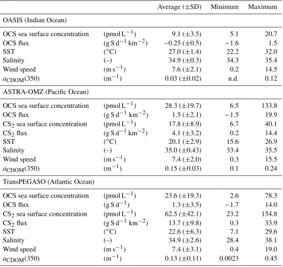
Table 3.Average, standard deviation and range of parameters observed during the cruises OASIS (Indian Ocean, 2014), ASTRA-OMZ (Pacific Ocean, 2015) and TransPEGASO (Atlantic Ocean, 2014).
Average (±SD) Minimum Maximum
OASIS (Indian Ocean)
OCS sea surface concentration (pmol L−1) 9.1 (±3.5) 5.1 20.7 OCS flux (g S d−1km−2) −0.25 (±0.5) −1.6 1.5
SST (◦C) 27.0 (±1.4) 22.2 32.0
Salinity (–) 34.9 (±0.3) 34.3 35.4
Wind speed (m s−1) 7.6 (±2.1) 0.2 14.5
aCDOM(350) (m−1) 0.03 (±0.02) n.d. 0.12
ASTRA-OMZ (Pacific Ocean)
OCS sea surface concentration (pmol L−1) 28.3 (±19.7) 6.5 133.8 OCS flux (g S d−1km−2) 1.5 (±2.1) −1.5 19.9 CS2sea surface concentration (pmol L−1) 17.8 (±8.9) 6.7 40.1
CS2flux (g S d−1km−2) 4.1 (±3.2) 0.2 14.4
SST (◦C) 20.1 (±2.9) 15.6 26.9
Salinity (–) 35.0 (±0.43) 33.4 35.5
Wind speed (m s−1) 7.4 (±2.0) 0.3 15.5
aCDOM(350) (m−1) 0.15 (±0.03) 0.1 0.24
TransPEGASO (Atlantic Ocean)
OCS sea surface concentration (pmol L−1) 23.6 (±19.3) 2.6 78.3
OCS flux (g S d−1) 1.3 (±3.5) −1.7 14.0
CS2sea surface concentration (pmol L−1) 62.5 (±42.1) 23.2 154.8
CS2flux (g S d−1km−2) 13.7 (±9.8) 0.3 33.9
SST (◦C) 22.6 (±6.3) 7.1 29.6
Salinity (–) 34.9 (±2.6) 28.4 38.1
Wind speed (m s−1) 7.4 (±3.1) 0.4 19.0
aCDOM(350) (m−1) 0.13 (±0.11) 0.0023 0.45
meridional transect (AMT-7) cruise (Kettle et al., 2001) (1.3– 112.0 pmol OCS L−1, mean 21.7 pmol OCS L−1).
Air–sea fluxes calculated from surface concentrations and mixing ratios of OCS as a function of wind speed gener-ally follow the diel cycle of the surface ocean concentration. While supersaturation prevailed during the day, low night-time concentrations usually led to oceanic uptake of atmo-spheric OCS. OCS fluxes integrated over one day ranged from−0.024 to−0.0002 g S km−2in the open Indian Ocean
and from 0.38 to 2.7 g S km−2in the coastal Pacific. During
the observed periods, the ocean was a net sink of atmospheric OCS in the Indian Ocean, whereas it was a net source in the eastern Pacific. Although an assessment of net flux is dif-ficult given the lower temporal resolution during TransPE-GASO, calculated emissions were in the same range as the ones measured in the Pacific and Indian Ocean.
The water masses encountered during the cruises to the Indian Ocean (OASIS) and eastern Pacific (ASTRA-OMZ), which are used to constrain the global box model, differ con-siderably with respect to the properties relevant for OCS cy-cling and, thus, span a large range of possible OCS
variabil-ity. The properties encountered during these two cruises en-compass or exceed the ones of the Pacific warm pool (cli-matological averages, Table 4), which is where the location of the missing source has been hypothesized (Glatthor et al., 2015; Kuai et al., 2015). Both higher SST and lower wind speeds (Table 4) would decrease the OCS sea surface con-centrations in the ocean, leading to decreased emissions to the atmosphere: higher SSTs favor a stronger degradation by hydrolysis (Elliott et al., 1989), and lower wind speeds de-crease the transfer velocityk. Lower integrated daily radia-tion (SR in Table 4) in the Pacific warm pool also points to lower OCS production. Hence, our new OCS observations presented here likely span the range of emission variability in the tropics.
Table 4. Comparison of water properties relevant for OCS production and consumption for the cruises OASIS (Indian Ocean, July– August 2014) and ASTRA-OMZ (eastern Pacific, October–November 2015) with the assumed source region in the Pacific warm pool (15◦N–15◦S, 120–180◦E). Data from cruises are in situ measurements; the data for the Pacific warm pool were extracted from climatolog-ical monthly means from sources for the global model run as specified in the Supplement.
Parameter OASIS ASTRA-OMZ Pacific warm pool
SST (◦C) 27.0±1.0 19.6±2.6 28.9±0.9
SSS (g kg−1) 35.0±0.3 35.1±0.3 34.5±0.42
Wind speed (m s−1) 8.2±1.7 7.5±1.8 5.3±0.4 a350(m−1) 0.039±0.02 0.146±0.02 0.050±0.08
I(W m−2) 226.5±303.0 196.4±283.1 206.4±286.6a
SR (J m−2) 1.9×10⁷±1.7×10⁶ 1.6×10⁷±4.5×10⁶ 8.9×10⁶±1.3×10⁶
pH (–) 8.03±0.01 –b 8.07±0.01
MLD (m) 43.3±15.8 18.9±7.5 35.9±14.1
aCalculated from an annual mean diurnal cycle based on ERA-Interim sunshine duration and flux. SR: surface radiation, daily
integral.bAssumed pH=8.15 for box model simulation.
3.2 A direct global oceanic emission estimate for OCS The OCS observations from the Indian and Pacific Ocean were used to improve a box model for simulating OCS con-centrations in the surface ocean (Kettle, 2002; Uher and Andreae, 1997b; von Hobe et al., 2003). With the a350
-dependent photoproduction constant included, the model re-produced the diel pattern of OCS concentrations in the sur-face oceans for both cruises (Fig. 2, black lines). A slight overestimation of observed concentrations is present for the Indian Ocean cruise OASIS (observed mean concentra-tion: 9.1±3.5 pmol L−1; simulated: 10.8
±3.9 pmol L−1).
This overestimation was more pronounced in the eastern Pacific (observed mean: 28.3±19.7 pmol L−1; simulated:
47.3±25.4 pmol L−1) and can largely be attributed to a lack
of downward mixing inherent in the mixed layer box model due to the assumption of the OCS concentration being con-stant throughout the entire mixed layer.
Using the linearp−a350parameterization for the first time
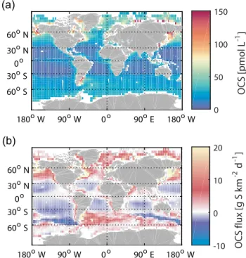
in a global model, the same box model as for the case studies is applied to estimate sea surface concentrations and fluxes of OCS on a global scale (Fig. 4). The OCS production is consistent with the global distribution of CDOM absorption (Fig. S5), with highest concentrations calculated for coastal regions and higher latitudes. Despite the photochemical hot spot in the tropics (30◦N–30◦S), degradation by hydrolysis prevents any accumulation of OCS in the surface water, as we calculated the lifetime due to hydrolysis to be only 7 h (Fig. S5). The simulated range of water concentrations is too low to sustain emissions in the tropics that could close the at-mospheric budget of OCS (Fig. 4). With saturation ratios in-tegrated over 1 year, the tropical ocean (30◦N–30◦S) is even undersaturated with respect to OCS, taking up 3.0 Gg S yr−1. Globally, the integration over one year yields annual oceanic OCS emissions of 130 Gg S. Our results corroborate the up-per limit of an earlier study that used an observation-derived emission inventory (Table 1) (Kettle, 2002) but which
180oW 90oE
0o 90oW 180oW 60oS 60oN
30oN 0o 30oS (a)
OCS [pmol L
-1 ]
0 50 100 150
180oW 90oE
0o 90oW 180oW 30oN
0o 30oS
60oS 60oN (b)
OCS flux [g S km
-2 d -1 ]
-10 0 10 20
Figure 4.Annual mean of surface ocean concentrations of OCS simulated with the box model(a)and corresponding emissions(b).
cludes more process-oriented parameterizations as described in Sect. 2.4. Clearly, our results from both observations and modeling contradict the latest bottom-up emission estimate from the NEMO-PISCES model (Launois et al., 2015a), and do not support a hot spot of direct OCS emissions in the Pa-cific Warm Pool or the tropical oceans in general.
3.2.1 Comparison to previous ship-based measurements
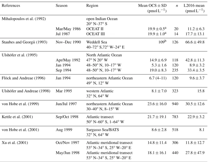
concen-Table 5.Comparison of previous ship campaign measurements with corresponding month and approximate geolocation from the global box model in this study (L2016), taken either from figures or tables as provided in the original references. Note that the box model is based on input data from climatological means that do not fully represent the conditions encountered during the respective cruises. Only observational data with measurements of the full diel cycle were included for comparison.n: number of measurements.
References Season Region Mean OCS±SD n L2016 mean
(pmol L−1) (pmol L−1)
Mihalopoulos et al. (1992) open Indian Ocean 20◦N–37◦S
Mar/May 1986 OCEAT II 19.9±0.5a 20 11.2±6.3
Jul 1987 OCEAT III 19.9±1.0a 14 17.7±13.1
Staubes and Georgii (1993) Nov–Dec 1990 Weddell Sea 109b 126 66.6±49.8 40–72◦S,72◦W–24◦E
Ulshöfer et al. (1995) North Atlantic Ocean
Apr/May 1992 47◦N 20◦W 14.9±6.9 118 42.8±11.3 Jan 1994 48–50◦N, 10–17◦W 5.3±1.6 120 8.9±3.2 Sep 1994 48–50◦N, 10–17◦W 19.0±8.3 235 33.4±3.5
Flöck and Andreae (1996) Jan 1994 northeastern Atlantic Ocean 6.7 (4–11) 120 9.6±3.7 49◦N, 12◦W
Ulshöfer and Andreae (1998) Mar 1995 western Atlantic 8.1±7.0 323 15.8 32◦N, 64◦W
von Hobe et al. (1999) Jun/Jul 1997 northeastern Atlantic Ocean 23.6±16.0 940 30.5±12.6 30–40◦N, 8–15◦W
Kettle et al. (2001) Sep/Oct 1998 Atlantic transect 21.7±19.1 783 22.9±3.2 50◦N–60◦S, 1–64◦W
von Hobe et al. (2001) Aug 1999 Sargasso Sea/BATS 8.6±2.8 518 8.1 32◦N, 64◦W
Xu et al. (2001) Oct/Nov 1997 Atlantic meridional transect 14.8±11.4 306 11.8±12.7 53◦N–34◦S, 25◦W–20◦E
May/Jun 1998 Atlantic meridional transect 18.1±16.1 440 27.8±47.9 53◦N–34◦S, 25◦W–20◦E
aConverted from ng L−1with a molar mass of OCS of 60.07 g.bConverted from ng S L−1with a molar mass ofSof 32.1 g.
trations (Table 5), the seasonal pattern of higher concentra-tions during summer compared to winter (as, for example, in Ulshöfer et al., 1995) and the spatial pattern of higher con-centrations in higher latitudes (e.g., Southern Ocean; Staubes and Georgii, 1993). Given that monthly means of a model simulation driven by climatological data of the input pa-rameters are compared to cruise measurements, the absolute mean deviation of 6.9 pmol L−1 and the mean deviation of
3.7 pmol L−1indicate an overall good reproduction of
obser-vations (differences between observation and model output were weighted to the number of observations in Table 4). It should be noted that, on average, the model overestimates OCS concentrations as indicated by the positive mean error, suggesting our emission estimate to be an upper limit to di-rect oceanic OCS emissions in most regions. The largest de-viations from observations are found in the Southern Ocean (see Staubes and Georgii, 1993, in Table 4), where the model underestimated observations by 40 %. While there are several
explanations for this, i.e., a possible violation of the under-lying assumption of a constant OCS production in regions with deep mixed layers such as the Southern Ocean, or the missing satellite data for CDOM during polar nights, it is a clear indication of the need for more observations from high latitudes. However, this underestimation does not interfere with our conclusion drawn for the tropical oceans, where the location of the missing source is derived from top-down ap-proaches.
3.2.2 Uncertainties
and especially in the tropical open ocean, where hydrolysis greatly exceeds surface outgassing and lowa350makes pho-toproduction extend further down in the water column, the model tends to overestimate the real OCS concentrations, as was shown for our two cruises above. Therefore, we deem the fluxes from our global simulation to represent an upper limit of the true fluxes. Only at high latitudes would we ex-pect more complex uncertainties, because hydrolysis at low temperatures is slow and only photoproduction and loss by outgassing are directly competing at the very surface.
Other uncertainties are associated with the calculation of the photoproduction rate. The wavelength of 443 nm com-bines the absorption of detritus and CDOM, which could have an impact especially in river plumes, where terrestrial material is transported into the ocean. As it is the CDOM that is important for photochemistry, assuming the 443 nm is purely CDOM would lead to an overestimation of photo-production and therefore is a conservative estimate. It should also be noted that a single spectral slope from 443 to 350 nm in the global simulation is a simplification. Furthermore, us-ing a wavelength integrated photoproduction rate constant in-stead of a wavelength-resolved approach, which would take global variations in the CDOM and light spectra into ac-count, is an additional simplification. It has been shown that this does not lead to large differences regionally (von Hobe et al., 2003) but could, potentially, lead to variations glob-ally. Ourp–CDOM relationship is a first step for constraing this variability globally in one parameterization, as it in-corporates photoproduction rate constants optimized to ob-servations and thus accounting for differences in the light and CDOM spectra. More data from different regions can help to further constrain this relationship in future studies. Despite these simplifications, the simulated concentrations agree very well with previous observations (n >4000, Ta-ble 4). To test the sensitivity of our box model to the pho-toproduction rate constant, we performed a sensitivity test with a photoproduction increased by a factor of 5 in the trop-ical region (30◦N–30◦S; note that this factor is considerably larger than the uncertainty in the p–CDOM relationship). This leads to an annual mean concentration of 35.1 pmol L−1
in the tropics (30◦N–30◦S), resulting in tropical direct emis-sions of 160 Gg S as OCS per year. The efficient hydrolysis in warm tropical waters prevents OCS concentrations from ac-cumulating despite the high photoproduction and still results in emissions too low to account for the missing source.
With a mean error of 3.7 pmol L−1in the OCS surface
wa-ter concentrations added to (subtracted from) the modeled concentration and subsequent calculation of fluxes using an-nual climatologies for wind, pressure and SST (same data sources as global simulation forcing data), we calculate an uncertainty of 60 %, which translates into a total uncertainty in the integrated global flux of 80 Gg S yr−1.
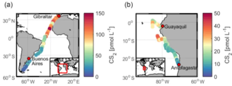
Figure 5.Measured concentration of CS2in surface waters during
(a)ASTRA-OMZ in the eastern Pacific Ocean and(b) TransPE-GASO in the Atlantic Ocean.
3.3 Indirect OCS emissions by DMS and CS2
A significant contribution to the OCS budget in the atmo-sphere results from oceanic emissions of DMS and CS2that
are partially converted to OCS on timescales of hours to days (Chin and Davis, 1993; Watts, 2000; Kettle, 2002). A yield of 0.7 % for OCS is used for the reaction of DMS with OH (Barnes et al., 1994), which results in a global oceanic source of DMS from OCS of 80 (65–110) Gg S yr−1 based on the procedure described in Sect. 2.5. The uncertainty range of 65–110 Gg S yr−1originated from the uncertainty in oceanic
emissions, not the conversion factor. This conversion fac-tor is much more uncertain, as the formation of OCS from DMS involves a complex multi-step reaction mechanism that is not fully understood. It has been shown in laboratory ex-periments that the presence of NOx reduces the OCS yield
considerably (Arsene et al., 2001), which would make our indirect emission estimate an upper limit. However, the yield was measured under laboratory conditions and may be dif-ferent and more variable under natural conditions.
DMS emissions do not show a pronounced hot spot in the Pacific warm pool region, but as DMS transports much more sulfur across the air–sea interface than OCS, even low changes in the OCS yield could affect the atmospheric budget of OCS. As the spatial oceanic emission pattern of DMS does not reflect the spatial pattern of the assumed missing source, a locally specific tropospheric change in the conversion yield would be one potential way of bringing the patterns in agree-ment. While it is possible that the OCS yield could vary un-der certain conditions (e.g., it cannot be excluded that the low OH concentrations in the broader Pacific warm pool area as suggested by Rex et al., 2014, influence the yield), the (lo-cal) increase in the conversion factor would need to be on the order of a factor of 10–100.
For CS2, the atmospheric reaction pathway producing
OCS is better understood with a well-constrained molar conversion ratio of 0.81 (Chin and Davis, 1993). However, the global distribution of oceanic CS2 concentration, and
hence its emissions to the atmosphere, is poorly known. In our study, surface CS2 concentrations (Fig. S6) were
on average 17.8±8.9 pmol L−1 during ASTRA-OMZ, and
latter values are higher than previously reported concentra-tions from the AMT-7 cruise in the central Atlantic (Ket-tle et al., 2001) (10.9±15.2 pmol L−1). We extrapolate a
weighted mean of the CS2 emissions from TransPEGASO
(n=42, 13.7±9.8 g S d−1km−2), ASTRA-OMZ (n=122, 4.1±3.2 g S d−1km−2) and AMT-7 (Kettle et al., 2001) (n=744, 1.6±1.8 g S d−1km−2) in order to estimate CS2
-derived OCS emissions from the global ocean. According to our extrapolation, 135 (7–260) Gg S yr−1enters the
atmo-sphere as oceanic CS2emissions converted to OCS. The
un-certainty range of 7–260 Gg S yr−1 results from
extrapolat-ing the highest and the lowest emissions encountered dur-ing the cruises to the global ocean. This number is at the highest end of the range for OCS emissions from globally simulated CS2oceanic concentrations (Kettle, 2000, 2002),
as measured CS2 concentrations from the cruises
ASTRA-OMZ and TransPEGASO are higher than the simulated sur-face concentrations in Kettle (2000) for the respective month. However, the spatial pattern of higher concentrations and emissions in the tropical region in our measurements agrees well with the spatial pattern simulated in Kettle (2000). Nonetheless, even the extrapolation of the highest measure-ment would not close the budget for the three largest missing source estimates (Table 1).
For oceanic emission estimates used to constrain GPP, quantifying the seasonal cycle of the single contributors is essential. For example, high emissions during oceanic spring and fall blooms could mask OCS uptake by the terrestrial vegetation, and therefore neglecting them could lead to an underestimation of global GPP, with implications for the at-mospheric and terrestrial carbon budget.
4 Conclusions and outlook
Considering the observational evidence and the modeled global emission estimate of 130±80 Gg S yr−1, direct OCS
emissions from the oceans are too low to account for the missing atmospheric source. Together with indirect emis-sions, the oceanic source strength of OCS would add up to 345 Gg S yr−1, compared to the 465–1089 Gg S yr−1
re-quired to balance the suggested increase in vegetation up-take. Direct and even additional indirect oceanic emissions of OCS are thus unlikely to balance the budget after the up-ward revision of the vegetation sink. Largest uncertainties are associated with the indirect emission estimates, especially in the conversion of DMS to OCS and the global source strength of CS2.
As our study suggests, the search for an additional source of OCS to the atmosphere should include other sources than oceanic emissions alone. There are indications of other parts of the OCS budget being underestimated, such as domes-tic coal combustion (Du et al., 2016). Emissions of biomass burning and direct and indirect anthropogenic emissions have been considered in previous estimates (e.g., 315.5 Gg S yr−1
in Berry et al., 2013, 224 Gg S yr−1in Kuai et al., 2015, and
219 Gg S yr−1 in Glatthor et al., 2015), but a recent
anthro-pogenic emission estimate by Lee and Brimblecombe (2016) increases this number to 598 Gg S yr−1, which would already bring sources and sinks closer to agreement. They attribute the largest direct OCS emissions to biomass and biofuel burning, as well as pulp and paper manufacturing, and the largest CS2emissions to the rayon industry. Hence, a hot spot
of anthropogenic emissions in the Asian continent might be a potential candidate, together with atmospheric transport, to produce atmospheric mixing ratios as observed by satellite.
A redistribution of the magnitude and seasonality of known sources and sinks could also bring top-down and bottom-up estimates closer together. For example, the gen-eral view of oxic soils as a sink for OCS has recently been challenged. Field (Maseyk et al., 2014; Billesbach et al., 2014) and incubation studies (Whelan et al., 2016) show that some oxic soils may shift from OCS uptake to emis-sion depending on the temperature and water content. Fur-thermore, it has been speculated previously that vegetation uptake might not be solely responsible for the decrease in OCS mixing ratios in fall because of the temporal lag be-tween CO2and OCS minimum (Montzka et al., 2007). The
observed seasonality in mixing ratios is a superposition of the seasonality of all individual sources and sinks. These season-alities are currently neglected or associated with a consider-able uncertainty. An improved understanding of the season-ality of the individual sources and sinks could help to better constrain the gap in the atmospheric budget. First steps to re-solve OCS seasonality in sources and sinks are currently be-ing undertaken, e.g., in the case of anthropogenic emissions (Campbell et al., 2015).
All in all, better constraints on the seasonality and magni-tude of the atmospheric OCS sources and sinks are critical for a better assessment of the role of this compound in cli-mate and its application to quantify GPP on a global scale. This study confirms oceanic emission as the largest known single source of atmospheric OCS but shows that its magni-tude is unlikely to balance the gap in the atmospheric OCS budget.
5 Data availability
All data, including OCS and CS2measurements in sea water
Appendix A: List of parameters
Symbol/abbreviation Meaning
a350 absorption coefficient of CDOM at 350 nm
a fitted parameter in diurnal cycle ofI b fitted parameter in diurnal cycle ofI cair concentration in air
COCS concentration of OCS in water F gas flux
H Henry constant
I downwelling solar radiation
K ion product of seawater
kw water-side transfer velocity in air–sea gas exchange
MLD mixed layer depth
p photoproduction rate constant SSS sea surface salinity
SST sea surface temperature
Sc Schmidt number
t time
θ zenith angle
u10 wind speed at 10 m height UV ultraviolet radiation
The Supplement related to this article is available online at doi:10.5194/acp-17-385-2017-supplement.
Acknowledgements. We thank the captain and crew of the research vesselsSONNEI and II as well asHesperidesfor assistance during the cruises SO235-OASIS (BMBF – FK03G0235A), SO243-ASTRA-OMZ (BMBF – FK03G0243A) and TransPEGASO. We thank H. W. Bange and A. Körtzinger for providing equipment for the continuous underway system and C. Schlundt for support dur-ing CS2measurements. This work was supported by the German Federal Ministry of Education and Research through the project ROMIC-THREAT (BMBF-FK01LG1217A and 01LG1217B) and ROMIC-SPITFIRE (BMBF-FKZ: 01LG1205C). Additional funding for Christa A. Marandino and Sinikka T. Lennartz came from the Helmholtz Young Investigator Group of Christa A. Marandino (TRASE-EC, VH-NG-819), from the Helmholtz As-sociation through the President’s Initiative and Networking Fund, and from the GEOMAR Helmholtz-Zentrum für Ozeanforschung Kiel. Kirstin Krüger acknowledges financial support from the EU FP7 StratoClim project (603557), and Pau Cortes and Rafel Simo acknowledge support from the Spanish MINECO through PEGASO (CTM2012-37615). We are grateful for the data provided by ECMWF (ERA-Interim) and NASA (MODIS-Aqua). DKRZ and its scientific steering committee are gratefully acknowledged for providing the HPC and data archiving resources for this consortial project ESCiMo (Earth System Chemistry Integrated Modelling). Elliott Atlas acknowledges support from the NASA Upper Atmosphere Research Program.
The article processing charges for this open-access publication were covered by a Research
Centre of the Helmholtz Association.
Edited by: S. Brown
Reviewed by: two anonymous referees
References
Andreae, M. O. and Ferek, R.: Photochemical production of car-bonyl sulfide in seawater and its emission to the atmosphere, Global Biogeochem. Cy., 6, 175–183, 2002.
Arévalo-Marténez, D. L., Beyer, M., Krumbholz, M., Piller, I., Kock, A., Steinhoff, T., Körtzinger, A., and Bange, H. W.: A new method for continuous measurements of oceanic and at-mospheric N2O, CO and CO2: performance of off-axis
inte-grated cavity output spectroscopy (OA-ICOS) coupled to non-dispersive infrared detection (NDIR), Ocean Sci., 9, 1071–1087, doi:10.5194/os-9-1071-2013, 2013.
Arneth, A., Harrison, S. P., Zaehle, S., Tsigaridis, K., Menon, S., Bartlein, P. J., Feichter, J., Korhola, A., Kulmala, M., O’Donnell, D., Schurgers, G., Sorvari, S., and Vesala, T.: Terrestrial biogeo-chemical feedbacks in the climate system, Nat. Geosci., 3, 525– 532, 2010.
Arsene, C., Barnes, I., Becker, K. H., and Mocanu, R.: FT-IR prod-uct study on the photo-oxidation of dimethyl sulphide in the
pres-ence of NOx – temperature dependence, Atmos. Environ., 35,
3769–3780, 2001.
Asaf, D., Rotenberg, E., Tatarinov, F., Dicken, U., Montzka, S. A., and Yakir, D.: Ecosystem photosynthesis inferred from measure-ments of carbonyl sulphide flux, Nat. Geosci., 6, 186–190, 2013. Asher, W. E. and Wanninkhof, R.: The effect of bubble-mediated gas transfer on purposeful dual-gaseous tracer experiments, J. Geophys. Res.-Ocean., 103, 10555–10560, 1998.
Atkinson, R., Baulch, D. L., Cox, R. A., Crowley, J. N., Hamp-son, R. F., Hynes, R. G., Jenkin, M. E., Rossi, M. J., and Troe, J.: Evaluated kinetic and photochemical data for atmospheric chem-istry: Volume I – gas phase reactions of Ox, HOx, NOxand SOx
species, Atmos. Chem. Phys., 4, 1461–1738, doi:10.5194/acp-4-1461-2004, 2004.
Barnes, I., Becker, K. H., and Patroescu, I.: The tropospheric ox-idation of dimethyl sulfide: A new source of carbonyl sulfide, Geophys. Res. Lett., 21, 2389–2392, 1994.
Beer, C., Reichstein, M., Tomelleri, E., Ciais, P., Jung, M., Carval-hais, N., Rödenbeck, C., Arain, M. A., Baldocchi, D., and Bonan, G. B.: Terrestrial gross carbon dioxide uptake: global distribution and covariation with climate, Science, 329, 834–838, 2010. Berry, J., Wolf, A., Campbell, J. E., Baker, I., Blake, N., Blake, D.,
Denning, A. S., Kawa, S. R., Montzka, S. A., Seibt, U., Stimler, K., Yakir, D., and Zhu, Z.: A coupled model of the global cy-cles of carbonyl sulfide and CO2: A possible new window on the
carbon cycle, J. Geophys. Res.-Biogeo., 118, 842–852, 2013. Billesbach, D. P., Berry, J. A., Seibt, U., Maseyk, K., Torn, M. S.,
Fischer, M. L., Abu-Naser, M., and Campbell, J. E.: Growing season eddy covariance measurements of carbonyl sulfide and CO2fluxes: COS and CO2relationships in Southern Great Plains
winter wheat, Agr. Forest Meteorol., 184, 48–55, 2014. Brown, K. A. and Bell, J. N. B.: Vegetation – The missing sink in
the global cycle of carbonyl sulphide (COS), Atmos. Environ., 20, 537–540, 1986.
Brühl, C., Lelieveld, J., Crutzen, P. J., and Tost, H.: The role of carbonyl sulphide as a source of stratospheric sulphate aerosol and its impact on climate, Atmos. Chem. Phys., 12, 1239–1253, doi:10.5194/acp-12-1239-2012, 2012.
Campbell, J. E., Carmichael, G. R., Chai, T., Mena-Carrasco, M., Tang, Y., Blake, D. R., Blake, N. J., Vay, S. A., Collatz, G. J., Baker, I., Berry, J. A., Montzka, S. A., Sweeney, C., Schnoor, J. L., and Stanier, C. O.: Photosynthetic Control of Atmospheric Carbonyl Sulfide During the Growing Season, Science, 322, 1085–1088, 2008.
Campbell, J. E., Whelan, M. E., Seibt, U., Smith, S. J., Berry, J. A., and Hilton, T. W.: Atmospheric carbonyl sulfide sources from anthropogenic activity: Implications for carbon cycle constraints, Geophys. Res. Lett., 42, 3004–3010, 2015.
Chin, M. and Davis, D. D.: Global sources and sinks of OCS and CS2 and their distributions, Global Biogeochem. Cy., 7, 321– 337, 1993.
Crutzen, P. J.: The possible importance of CSO for the sulfate layer of the stratosphere, Geophys. Res. Lett., 3, 73–76, 1976. De Bruyn, W., Swartz, E., Hu, J., Shorter, J., Davidovits, P.,
Dee, D. P., Uppala, S. M., Simmons, A. J., Berrisford, P., Poli, P., Kobayashi, S., Andrae, U., Balmaseda, M. A., Balsamo, G., Bauer, P., Bechtold, P., Beljaars, A. C. M., van de Berg, L., Bid-lot, J., Bormann, N., Delsol, C., Dragani, R., Fuentes, M., Geer, A. J., Haimberger, L., Healy, S. B., Hersbach, H., Hólm, E. V., Isaksen, L., Kållberg, P., Köhler, M., Matricardi, M., McNally, A. P., Monge-Sanz, B. M., Morcrette, J. J., Park, B. K., Peubey, C., de Rosnay, P., Tavolato, C., Thépaut, J. N., and Vitart, F.: The ERA-Interim reanalysis: configuration and performance of the data assimilation system, Q. J. Roy. Meteor. Soc., 137, 553–597, 2011.
de Gouw, J. A., Warneke, C., Montzka, S. A., Holloway, J. S., Par-rish, D. D., Fehsenfeld, F. C., Atlas, E. L., Weber, R. J., and Flocke, F. M.: Carbonyl sulfide as an inverse tracer for biogenic organic carbon in gas and aerosol phases, Geophys. Res. Lett., 36, L05804, doi:10.1029/2008GL036910, 2009.
Dickinson, A. G. and Riley, J.: The estimation of acid dissociation constants in seawater media from potentiometric titrations with strong base, Mar. Chem., 7, 89–99, 1979.
Du, Q., Zhang, C., Mu, Y., Cheng, Y., Zhang, Y., Liu, C., Song, M., Tian, D., Liu, P., Liu, J., Xue, C., and Ye, C.: An im-portant missing source of atmospheric carbonyl sulfide: Do-mestic coal combustion, Geophys. Res. Lett., 43, 8720–8727, doi:10.1002/2016GL070075, 2016.
Elliott, S., Lu, E., and Rowland, F. S.: Rates and mechanisms for the hydrolysis of carbonyl sulfide in natural waters, Environ. Sci. Tech., 23, 458–461, 1989.
Ferek, R. and Andreae, M. O.: The supersaturation of carbonyl sul-fide in surface waters of the pacific oceans off Peru, Geophys. Res. Lett., 10, 393–395, 1983.
Ferek, R. and Andreae, M. O.: Photochemical production of car-bonyl sulphide in marine surface waters, Letters to Nature, 1984, 148–150, 1984.
Fichot, C. G. and Miller, W. L.: An approach to quantify depth-resolved marine photochemical fluxes using remote sensing: Ap-plication to carbon monoxide (CO) photoproduction, Remote Sens. Environ., 114, 1363–1377, 2010.
Flöck, O. and Andreae, M. O.: Photochemical and non-photochemical formation and destruction of carbonyl sulfide and methyl mercaptan in ocean waters, Mar. Chem., 54, 11–26, 1996. Flöck, O. R., Andreae, M. O., and Dräger, M.: Environmentally relevant precursors of carbonyl sulfide in aquatic systems, Mar. Chem., 59, 71–85, 1997.
Glatthor, N., Höpfner, M., Baker, I. T., Berry, J., Campbell, J. E., Kawa, S. R., Krysztofiak, G., Leyser, A., Sinnhuber, B. M., Stiller, G. P., Stinecipher, J., and Clarmann, T. V.: Tropical sources and sinks of carbonyl sulfide observed from space, Geo-phys. Res. Lett., 42, 10082–10090, doi:10.1002/2015GL066293, 2015.
Hayduk, W. and Laudie, H.: Prediction of diffusion coefficients for nonelectrolytes in dilute aqueous solutions, AIChE Journal, 20, 611–615, 1974.
Jöckel, P., Tost, H., Pozzer, A., Kunze, M., Kirner, O., Brenninkmei-jer, C. A. M., Brinkop, S., Cai, D. S., Dyroff, C., Eckstein, J., Frank, F., Garny, H., Gottschaldt, K.-D., Graf, P., Grewe, V., Kerkweg, A., Kern, B., Matthes, S., Mertens, M., Meul, S., Neu-maier, M., Nützel, M., Oberländer-Hayn, S., Ruhnke, R., Runde, T., Sander, R., Scharffe, D., and Zahn, A.: Earth System Chem-istry integrated Modelling (ESCiMo) with the Modular Earth
Submodel System (MESSy) version 2.51, Geosci. Model Dev., 9, 1153–1200, doi:10.5194/gmd-9-1153-2016, 2016.
Johnson, J. E. and Harrison, H.: Carbonyl Sulfide Concentrations in the Surface Waters and Above the Pacific Ocean, J. Geophys. Res., 91, 7883–7888, 1986.
Kettle, A.: Extrapolations of the Flux of Dimethylsulfide, Carbon Monooxide, Carbonyl Sulfide and Carbon Disulfide from the Oceans, PhD thesis, 2000.
Kettle, A. J.: Global budget of atmospheric carbonyl sulfide: Tem-poral and spatial variations of the dominant sources and sinks, J. Geophys. Res., 107, 4658, doi:10.1029/2002JD002187, 2002. Kettle, A. J., Rhee, T. S., von Hobe, M., Poulton, A., Aiken, J.,
and Andreae, M. O.: Assessing the flux of different volatile sul-fur gases from the ocean to the atmosphere, J. Geophys. Res.-Atmos., 106, 12193–12209, 2001.
Kremser, S., Jones, N. B., Palm, M., Lejeune, B., Wang, Y., Smale, D., and Deutscher, N. M.: Positive trends in Southern Hemi-sphere carbonyl sulfide, Geophys. Res. Lett., 42, 9473–9480, 2015.
Kremser, S., Thomason, L. W., von Hobe, M., Hermann, M., Desh-ler, T., Timmreck, C., Toohey, M., Stenke, A., Schwarz, J. P., Weigel, R., Fueglistaler, S., Prata, F. J., Vernier, J.-P., Schlager, H., Barnes, J. E., Antuña-Marrero, J.-C., Fairlie, D., Palm, M., Mahieu, E., Notholt, J., Rex, M., Bingen, C., Vanhellemont, F., Bourassa, A., Plane, J. M. C., Klocke, D., Carn, S. A., Clarisse, L., Trickl, T., Neely, R., James, A. D., Rieger, L., Wil-son, J. C., and Meland, B.: Stratospheric aerosol – Observations, processes, and impact on climate, Rev. Geophys., 54, 278–335, doi:10.1002/2015RG000511, 2016.
Kuai, L., Worden, J. R., Campbell, J. E., Kulawik, S. S., Li, K.-F., Lee, M., Weidner, R. J., Montzka, S. A., Moore, F. L., Berry, J. A., Baker, I., Denning, A. S., Bian, H., Bowman, K. W., Liu, J., and Yung, Y. L.: Estimate of carbonyl sulfide tropical oceanic surface fluxes using Aura Tropospheric Emission Spectrome-ter observations, J. Geophys. Res.-Atmos., 120, 11012–11023, 2015.
Lana, A., Bell, T. G., Simo, R., Vallina, S. M., Ballabrera-Poy, J., Kettle, A. J., Dachs, J., Bopp, L., Saltzman, E. S., Ste-fels, J., Johnson, J. E., and Liss, P. S.: An updated climatology of surface dimethlysulfide concentrations and emission fluxes in the global ocean, Global Biogeochem. Cy., 25, GB1004, doi:10.1029/2010GB003850, 2011.
Launois, T., Belviso, S., Bopp, L., Fichot, C. G., and Peylin, P.: A new model for the global biogeochemical cycle of carbonyl sulfide – Part 1: Assessment of direct marine emissions with an oceanic general circulation and biogeochemistry model, At-mos. Chem. Phys., 15, 2295–2312, doi:10.5194/acp-15-2295-2015, 2015a.
Launois, T., Peylin, P., Belviso, S., and Poulter, B.: A new model of the global biogeochemical cycle of carbonyl sulfide – Part 2: Use of carbonyl sulfide to constrain gross primary productivity in current vegetation models, Atmos. Chem. Phys., 15, 9285–9312, doi:10.5194/acp-15-9285-2015, 2015.
Lee, C.-L. and Brimblecombe, P.: Anthropogenic contributions to global carbonyl sulfide, carbon disulfide and organosulfides fluxes, Earth-Sci. Rev., 160, 1–18, 2016.