Oceanic tracer and proxy time scales revisited

(1)

CPD

6, 1589–1628, 2010

Oceanic tracer and proxy time scales

revisited

C. Siberlin and C. Wunsch

Title Page

Abstract Introduction

Conclusions References

Tables Figures

◭ ◮

Back Close

Full Screen / Esc

Printer-friendly Version Interactive Discussion

Discussion

P

a

per

|

Dis

cussion

P

a

per

|

Discussion

P

a

per

|

Discussio

n

P

a

per

|

Clim. Past Discuss., 6, 1589–1628, 2010 www.clim-past-discuss.net/6/1589/2010/ doi:10.5194/cpd-6-1589-2010

Climate of the Past Discussions

This discussion paper is/has been under review for the journal Climate of the Past (CP). Please refer to the corresponding final paper in CP if available.

Oceanic tracer and proxy time scales

revisited

C. Siberlin and C. Wunsch

Department of Earth, Atmospheric and Planetary Sciences, Massachusetts Institute of Technology, Cambridge, MA 02139, USA

Received: 9 August 2010 – Accepted: 11 August 2010 – Published: 1 September 2010 Correspondence to: C. Wunsch (cwunsch@mit.edu)

(2)

CPD

6, 1589–1628, 2010

revisited

Title Page

Tables Figures

◭ ◮

Back Close

Full Screen / Esc

Discussion

P

a

per

|

Dis

cussion

P

a

per

|

Discussion

P

a

per

|

Discussio

n

P

a

per

|

Abstract

Quantifying time-responses of the ocean to passive and active tracers is critical for the interpretation of paleodata from sediment cores because surface-injected tracers do not instantaneously spread throughout the ocean. To obtain insights into the time response, a computationally efficient state transition matrix method is demonstrated

5

and used to compute successive states of passive tracer concentrations in the global ocean. Times to equilibrium exceed a thousand years for any one region of the global ocean outside of the injection and convective regions and concentration gradients give time-lags from hundreds to thousands of years between the Atlantic and Pacific abyss, depending on the injection region and the nature of the boundary conditions employed.

10

Equilibrium times can be much longer than radiocarbon ages as the latter are strongly biased towards the youngest fraction of fluid captured in a sample. Pulse-like inputs can produce very different transient approaches to equilibrium in different parts of the ocean generating event identification problems.

1 Introduction 15

In a recent paper, Wunsch and Heimbach (2008; hereafter WH08) studied the re-sponse of an oceanic general circulation model (GCM) to a passive tracer entering at the sea surface. Their stated intention was to obtain order of magnitude estimates of the time it takes such tracers to reach equilibrium – a time important to understand-ing climate change signals appearunderstand-ing in di_fferent parts of the ocean. The study was

20

stimulated in part by the paper of Skinner and Shackleton (2005) that concluded that apparent phase delays between perceived signals in the abyssal North Atlantic and North Pacific Oceans could only be explained if the circulation had shifted while the proxy transient was taking place. WH08 concluded that the response times for signal propagation from one part of the ocean to another were by themselves large enough to

25

(3)

CPD

6, 1589–1628, 2010

revisited

Title Page

Tables Figures

◭ ◮

Back Close

Full Screen / Esc

Discussion

P

a

per

|

Dis

cussion

P

a

per

|

Discussion

P

a

per

|

Discussio

n

P

a

per

|

of course, does not preclude changes in the circulation – which wouldnecessarily oc-cur under any climate change.) Lea et al. (2000) is another example of a study in which the apparent time lag between a regional temperature change, and the arrival of the signature of deglaciation, is used to infer a causal link. Of particular concern in the study of deep-sea cores is the oceanic adjustment to the sometimes extremely strong

5

signature of changes in ice volume entering the ocean as a freshwater flux carrying e.g.,δ18O, signatures that eventually influence the entire ocean.

Although the intention of WH08 was simply to gain an understanding of the time scales present in the oceanic adjustment process to tracer input, their inferences were subsequently criticized by Primeau and Deleersnijder (2009; hereafter PD09) who point

10

out that a surfaceflux (Neumann) boundary condition could produce distributions ex-hibiting an appreciably shorter equilibrium time than that found by WH08 using a con-centration (Dirichlet) condition. For many of the proxies of paleoceanographic interest, there is little doubt that surface flux rather than surface concentration boundary condi-tions are more appropriate. On the other hand, it is also apparent that such boundary

15

conditions can lead tolonger adjustment times – as we will discuss – and that studies of equilibrium under such circumstances are necessarily somewhat more complex.

A considerable literature has grown up in recent years around the general, mainly theoretical, problems of the interpretation of tracer data. Much of the focus of that litera-ture (see e.g., Waugh et al., 2003, for many earlier references), has been in the context

20

of what are labelled “travel time distributions” in which the distribution of water mass origins at different points are treated as though they are stochastic variables derived from a probability density (the travel time distribution). That point of view is an inter-esting one, but implies an underlying stochastic physics distinct from any deterministic quasi-steady-state. In practice, “travel time distributions” are known to a much broader

25

(4)

CPD

6, 1589–1628, 2010

revisited

Title Page

Tables Figures

◭ ◮

Back Close

Full Screen / Esc

Discussion

P

a

per

|

Dis

cussion

P

a

per

|

Discussion

P

a

per

|

Discussio

n

P

a

per

|

(some of them are very powerful tools in analyzingmodel calculations of tracers), it is not obvious that the use of real tracers in paleoceanography is rendered easier by their employ. Because of the importance of proxy tracers in paleoclimate, and in keeping with the purpose of WH08 as primarily providing a rough guide to interpreting tracers, it is worthwhile revisiting this subject to summarize those inferences that are likely to

5

be robust. Much of what is here derives from the recent thesis of Siberlin (2010) and is intended in part as a tutorial: many of the inferences here are scattered through a not-always-transparent technical literature. We endeavor to employ as little mathematics as is practical, and some of the details have been put into an appendix.

For context, consider a global ocean of volume, V. It is supposed that the three

10

dimensional water circulation withinV is known (it can be time-dependent) as are any mixing coefficients. A passive tracer, C(one not affecting the water density or its dy-namical properties), is introduced at the sea surface of the volume, and supposed to satisfy a conventional advection-di_ffusion equation of the form,

∂C

∂t +v·∇C−∇(K∇C)=q, (1)

15

wherev(r,t)=[u,v,w] is the three-dimensional flow field, K is a mixing tensor, and q

represents interior sources or sinks including, where appropriate, decay terms such as

q=−λCas in14C._∇is the three-dimensional gradient operator,_∇=

∂/∂x,∂/∂y,∂/∂z

(in practice, one uses spherical coordinates). r₌[x,y,z] is a generic position vector. (Isotopic ratios do not satisfy this equation: instead the numerator and denominator

20

separately satisfy one like it, with the ratio itself being described by a complex non-linear relationship.)

Ages

Most of the paleotracer community has relied not upon equilibrium times as discussed by WH08, but upon radiocarbon ages, which in general prove considerably shorter.

25

(5)

CPD

6, 1589–1628, 2010

revisited

Title Page

Tables Figures

◭ ◮

Back Close

Full Screen / Esc

Discussion

P

a

per

|

Dis

cussion

P

a

per

|

Discussion

P

a

per

|

Discussio

n

P

a

per

|

in various definitions and interpretations. Gebbie and Huybers (2010b) provide an overview and many earlier references. For the moment, consider only the very simple case of a water sample, perhaps one in the deep South Pacific, made up of N fluid parcels of equal volume which left the sea surface at a variety of times, ti, before

forming the measured sample. In the transit time distribution point of view, theti are 5

selected from a probability density function, but as already noted, this interpretation is not a necessary one, and here they are regarded as values fixed at any observation point. For maximum simplicity, assume further that the surface starting concentration of radiocarbon is identical, C0, in all components, and that there is no exchange by

diffusion or other process along the pathway to the observation location. Then the

10

radiocarbon concentration, when measured, is

Cobs=

1

N

C0e−λt1+C0e−λt2+...+C0e−λtN

,

whereλ≈1/5730 yr is the radiocarbon decay constant. The true mean age, ¯τ, would be the ordinary average of the arrival times,

¯

τ= 1

N N

X

i=1

t_i. (2)

15

The radiocarbon age is

τRC=−

1

λln

_C

obs C0

=−1

λln

h

e−λt1₊_...₊_e−λtN

.

Ni.

If there is only one time of arrival, τRC=τ.¯ With two arrivals, τRC<τ¯, because

exp(₋λt2)<exp(−λt1). The radiocarbon age is biassed, perhaps strongly so, towards

the age of the most recent arrival – concentrations from later arrivals giving strongly

20

downweighted contributions. If the second arrival took much longer than the radio-carbon decay time, so thatC0exp(−λt2)≈0, thenτRC=t1 and the potential difference

(6)

CPD

6, 1589–1628, 2010

revisited

Title Page

Tables Figures

◭ ◮

Back Close

Full Screen / Esc

Discussion

P

a

per

|

Dis

cussion

P

a

per

|

Discussion

P

a

per

|

Discussio

n

P

a

per

|

large. Various simple examples of this bias error can be worked out from assumptions about travel time values (see the references), but which we do not pursue here. In this same situation, one can define the approach to equilibrium for a stable tracer by noting that if fluid arrives at the observation point where the initial concentration isC=0,then it will rise toward its final concentration ofC0according to,

5

C(t)=C0

N (t1+t2+...+tf), tf≤tN,

the full value being obtained only after the last contribution has arrived (assuming the

t_i are in increasing order). If, following WH08, effective equilibrium is arbitrarily defined as the time when C(t)=0.9C0, then t90 will always exceed ¯τ, the mean time, and ¯τ

will always exceedτRC. (Equilibrium times are discussed further below.) This bias is 10

well known in the context of numerical model “ideal tracer ages” (e.g., Khatiwala et al., 2001). The degree of bias, and hence the apparent age, depends upon λ,and so is a property of the tracer and not just the fluid.

The main message is that,assuming the initial surface values of C are not greatly different, one expects calculated tracer ages to be systematically less than true mean

15

ages, sometimes greatly so, and that they should prove considerably shorter than equi-librium times, is no particular surprise. If the values of thet_i were known, as they can be in a numerical model, one can account for the bias. But with isolated radiocarbon data alone, it is not possible. The investigator using these ages must be clear on the phys-ical meaning of the different ages and the context in which they are being employed.

20

WD08 used equilibrium times because tracer concentrations appear in the advection-diffusion equation as spatial and temporal gradients; the use of disequilibrium values in a steady-state can introduce major errors and produce misleading inferences about travel time differences of tracer anomalies, or rates of biological productivity or rem-ineralization.

25

(7)

CPD

6, 1589–1628, 2010

revisited

Title Page

Tables Figures

◭ ◮

Back Close

Full Screen / Esc

Discussion

P

a

per

|

Dis

cussion

P

a

per

|

Discussion

P

a

per

|

Discussio

n

P

a

per

|

situation would be much more extreme for shorter-lived isotopes such as tritium. (See Gebbie and Huybers, 2010b for further discussion and references.) If two water parcels produce radiocarbon ages in which one is younger than the other, little can be inferred directly about the time-mean age. Because water parcels will not travel unchanged from the surface, but will exchange diffusively with their surroundings along potentially

5

very long trajectories, the real situation is actually far more complex. Radiocarbon ages will be discussed a bit more below.

Time scales

Tracer problems in three-dimensions, satisfying equations such as Eq. (1), produce a multiplicity of time scales and which can and will appear in the solutions and,

de-10

pending upon their magnitudes, determine the structure of the oceanic response. Let the volume,V,under consideration have cross-sectionL,and depthD.If one assumes, for maximum simplicity, thatKis composed solely of a spatially and temporally constant vertical component,K_z,and horizontal component,K_x,diffusion coefficients, then out of the equation one can construct numerous time scales (see e.g., Wunsch, 2002)

in-15

cluding, T1=D 2

/K_z, T2=L 2

/K_x, T3=D/w, T4=1/λ,(there are others). Mathematically,

the ultimate equilibrium of an advection-diffusion process, as in Eq. (1), is always con-trolled by the di_ffusive terms, which ultimately erase the strong gradients sometimes generated by the advective ones. In any complete solution to Eq. (1), one expectsall

of these timescales to appear. Whether they are of any practical significance to

some-20

one interpreting that solution depends upon the problem details. If the tracer were tritium, with a half-life of about 12 yr, injected into the North Atlantic alone, the solution in the deep North Pacific would include terms involvingT2≈2000 yr. But as the

concen-tration in the deep Pacific would always be vanishingly small,T2would be irrelevant in

practice. If the tracer were, however,14C, with a half-life of about 5730 yr, the longest

25

of the internal time scalesT_i would likely be of concern. In general these time scales aree-folding times, representing achievement of about 65% of any final value.

(8)

CPD

6, 1589–1628, 2010

revisited

Title Page

Tables Figures

◭ ◮

Back Close

Full Screen / Esc

Discussion

P

a

per

|

Dis

cussion

P

a

per

|

Discussion

P

a

per

|

Discussio

n

P

a

per

|

a general circulation model (GCM) to 14 yr of global oceanic data sets, and ran it in a perpetual loop for about 1900 yr. Tracers were introduced in a series of numerical experiments to determine time scales in which near-equilibrium could be obtained. That is, a concentration of C=1 (conceptually, a red dye, and we will refer to it as “dye”) was introduced at the sea surface at time t=0, in one instance over the entire

5

surface area, B, of the global ocean, and held fixed. In other experiments, a sub-area,B₁, such as the northern North Pacific or North Atlantic was introduced and held fixed. In the remaining, undyed, surface area, a condition of no flux to the atmosphere was imposed. The purpose of this latter requirement was to prevent dye from being exchanged with the atmosphere outside of the input region so that all of it remained

10

within the ocean. With the dye being conserved in the ocean, one could then infer, without actually computing it, that the final equilibrium state would be a globally uniform value ofC=1 everywhere in a steady-state (the whole ocean would be dyed red).

Although no analytical solution to Eq. (1) is available, one expects all of the adjust-ment times,T_i,to be present at every location in the ocean, with a solution structure in

15

which different regions would be dominated by one or more, but differing, time scales. For example, in a solution in which the dye was introduced only in the northern North Atlantic, one might expect that below the surface there, in a region of Ekman down-welling that the solution would be controlled by D/w, in a potentially very rapid re-sponse. In contrast, in a region of Ekman upwelling, the main time scale might be the

20

diffusive one,D2/K_z. In the remote Pacific, the dominant time scale could be horizon-tal diffusion, L2/K_x. To provide a simple diagnostic of the many time scales, WH08 used the “90% equilibrium time”,t90,as a measure of the time to equilibrium. That is,

with the knowledge that the final steady-state isC=1,always reached from below, one could map the time when 90% of this value was obtained in the solution.

25

As they discuss, however, the time to full equilibrium is formally infinite, and the choice oft90 is largely arbitrary: the appropriate value depends upon one’s goals. In

more complex boundary value problems, the final equilibrium concentration, C_∞(r),

(9)

CPD

6, 1589–1628, 2010

revisited

Title Page

Tables Figures

◭ ◮

Back Close

Full Screen / Esc

Discussion

P

a

per

|

Dis

cussion

P

a

per

|

Discussion

P

a

per

|

Discussio

n

P

a

per

|

version of an equation such as Eq. (1) for the purpose e.g., of determining,K_z.A 10% error in the true equilibrium value might be tolerable. A di_fferent error might be ac-ceptable if e.g., the problem is determining the global inventory of C at equilibrium. For some other problems, one might require the time of first arrival of measurable tracer at a distant location as a measure of a “signal velocity”. Such a use evidently

5

depends upon the measurement capability translated into a detection threshold. A sim-ilar dependence upon measurement accuracies and precisions could dictate a different equilibrium level determination. That is, if measurement technology cannot distinguish betweenC=0.9 andC=1,there would be little point in usingt98.

Additional, practically important, time scales are those imposed by the boundary

10

data – e.g., the time duration of a pulse of tracer and/or whether it is strongly seasonal – be it from a concentration or flux boundary conditions. Whether the boundary con-ditions or the circulation remain steady-enough to render discussion of equilibrium of relevance can only be decided on a case-by-case basis. This problem, of interpret-ing tracer data, involves an intricate couplinterpret-ing of goals, mathematics, and observational

15

capability, and the comparatively crude time scales such as those produced by either WH08 or PD09 are mainly part of the qualitative background information useful when constructing interpretations.

2 External time scales

The WH08 solutions depend only upon theinternal time scales, Ti, of the problem. 20

In the pulse injection solutions of PD09, anexternal time scale,Text,was necessarily

introduced. That is, if dye is injected at a fixed rate, rather than imposed as fixed surface concentration, and if it is similarly conserved within the ocean, there is no final steady equilibrium. Instead, the final state would be a growing concentration,

C(r,t)∼A(r)t. (3)

(10)

CPD

6, 1589–1628, 2010

revisited

Title Page

Tables Figures

◭ ◮

Back Close

Full Screen / Esc

Discussion

P

a

per

|

Dis

cussion

P

a

per

|

Discussion

P

a

per

|

Discussio

n

P

a

per

|

To avoid this situation, PD09 defineTextsuch that, TextF0B1=C∞V,

whereF0 is the rate of injection,B1 is the area of injection, andC∞=1.That is, given

F0,Textis chosen so that the total amount of injected dye is exactly that value producing

a total final ocean concentration ofC=1 uniformly everywhere – as before. Once again,

5

the final concentration, when reached, will be uniform and the total injected dye will be exactly the same as obtained from the concentration boundary conditions of WH08.

That such a pulse can lead to a rather different temporal behavior is readily seen by choosingText=1 yr. All of the dye comes in e.g., in the North Atlantic, in one year

(perhaps by a glacial ice-melt event) Such an injected pulse will build up relatively very

10

large concentration values in the North Atlantic in such a way that in and near that re-gion, all of the terms of Eq. (1) involving spatial derivatives such as∂C/∂y,∂2C/∂z2,

can become extremely large, and hence greatly increasing regional values of∂C/∂t. Regionally, the time to reach C=1 can be extremely small (albeit the space-time his-tory, as shown below, is sometimes complex – involving overshoots of the final

con-15

centration value). It is this increase in regional derivatives that underlies the shortened timescales seen by PD09. Note that in the concentration problem of WH08, the value ofC nowhere ever exceedsC=1,and thus the gradients of Care clearly bounded by (C=1)−(C=0)=1, while no such bound applies in the flux case. (A dependence upon area,B₁,is also present, but that will not be explored here.)

20

(11)

CPD

6, 1589–1628, 2010

revisited

Title Page

Tables Figures

◭ ◮

Back Close

Full Screen / Esc

Discussion

P

a

per

|

Dis

cussion

P

a

per

|

Discussion

P

a

per

|

Discussio

n

P

a

per

|

3 Some illustrative experiments

As the purpose of this paper is to provide some further insight into the evolution of proxy tracers, it is helpful to explore some solutions under a variety of boundary con-ditions, including those of WH08 and PD09. Computation over thousands of years in a realistic ocean circulation of tracers obeying equations such as Eq. (1) remains

com-5

putationally non-trivial. WH08 used a so-called online version of the full GCM code and limited themselves to 1900 yr – exploiting their knowledge of the final equilibrium state. Here we use a computationally efficient scheme made possible by the so-called state transition matrix determined for the same GCM by Khatiwala et al. (2005) and Khati-wala (2007). Some additional approximations are made using this form, and so one

10

chore is to demonstrate that solutions do not qualitatively differ from those of WH08 (orders of magnitude effects still being the focus).

3.1 The state transition matrix

Equation (1) is a linear system, and as such (e.g., Brogan, 1991; Wunsch, 2006) it can be written, very generally, in so-called state vector form,

15

x(t+ ∆t)=A(t)x(t)+Bq(t), (4)

wherex(t),the state-vector, is the vector of concentrations at every grid point at dis-crete time,t. The “state transition matrix”, A(t), can be derived from the GCM code normally used to calculateC(t) (Khatiwala et al., 2005), and others, discussing tran-sit time distributions, usually call it the “transport matrix”; we prefer our more generic

20

terminology – which is widely used in the control literature. Note also that in oceanog-raphy, “transport” is often assumed to denote, specifically, the advective component, not including the diffusive part.). Bq(t) is, in the notation of Wunsch (2006), a general representation of the boundary conditions and sources. The representation is appli-cable, by increasing the state vector dimension, for models using implicit calculations

25

(12)

of-CPD

6, 1589–1628, 2010

revisited

Title Page

Tables Figures

◭ ◮

Back Close

Full Screen / Esc

Discussion

P

a

per

|

Dis

cussion

P

a

per

|

Discussion

P

a

per

|

Discussio

n

P

a

per

|

tenBq(t)_→Bq_∞, a constant vector. Suppose that this system is time-stepped until a steady-state is reached. Then,

x(t+ ∆t)=x(t)=x_∞ (5)

and it must be true from Eq. (4) that,

x_∞₌A(t)x_∞₊Bq_∞. (6)

5

If a steady-state does emerge, the time variations in A(t) must become sufficiently small that it too can be treated as a constant,A_∞. Then it follows immediately (e.g., Brogan; 1991, Wunsch, 2006),

x_∞=(I−A_∞)−1Bq_∞. (7)

That is, the final, asymptotic state can be computed through the inversion of a single,

10

very sparse, matrix (equivalently, from the solution of a very sparse set of simultaneous equations). Although the matrix is available at climatological monthly intervals, for present purposes its annual mean value is used. That approximation removes some of the physics of wintertime convection, and it is necessary to confirm that, among other approximations, it does not greatly modify the time scales.

15

Although it is not the primary interest here, it is useful to briefly explore steady-states more structured than the simple one used by WH08. Thus, we exploit the availability of the state transition matrix provided to us by S. Khatiwala (personal communica-tion, 2009, 2010) and based upon the same ECCO model as used by WH08. A is found by computing numerical Green function solutions from a 2.8◦ horizontal

resolu-20

tion, 15-vertical layer, configuration of the MITgcm with a 20 min time-step, and forced with monthly mean climatological fluxes of momentum, heat and freshwater. Some additional model details are provided in the Appendix. Consider, by way of example, a system in which a large North Atlantic region (see Fig. 1) is dyed (a concentration boundary condition held fixed), but with the concentration set toC=0 outside that area.

25

(13)

CPD

6, 1589–1628, 2010

revisited

Title Page

Tables Figures

◭ ◮

Back Close

Full Screen / Esc

Discussion

P

a

per

|

Dis

cussion

P

a

per

|

Discussion

P

a

per

|

Discussio

n

P

a

per

|

maintain the values imposed.) The final steady-state concentration is no longer uni-form (see Fig. 2). This use of the state transition matrix, with any boundary condition, would be important in helping to interpret tracers believed at equilibrium.

In addition, usingA,the time stepping solutions of Eq. (4) can also be obtained very rapidly. The goal remains the same as in WH08: to obtain order of magnitude estimates

5

of the time required for a passive tracer to come close to equilibrium under transient forcing. We emphasize that solution details are not the focus of attention, as it would be di_fficult to defend a circulation remaining fixed over thousands of years. One can regard the results that follow as an elaborate scale analysis of the ocean circulation, one believed semi-quantitatively correct, and so useful as a guideline in interpreting

10

proxy and other tracer data.

Although a variety of experiments is discussed by Siberlin (2010), we confine this dis-cussion to a subset involving inputs restricted to the North Atlantic and North Pacific. It proves convenient to discuss three distinct boundary conditions: (1) Concentration-step (Dirichlet-Heaviside) in which the concentration at the sea surface is fixed atC=1

15

and held there indefinitely. Outside this region, there is no atmospheric flux, thus con-serving total tracer entering the ocean (WH08). (2) Flux-step (Neumann-Heaviside) in which a flux boundary condition is imposed in some region and held there indefinitely. No tracer transfer back to the atmosphere is permitted anywhere and no steady state exists. (3) Flux-pulse (Neumann-pulse) in which the flux of (2) is re-set to zero after

20

t=Text, and where the total injected tracer is identical to that in (1) after infinite time

(PD09). We will not discuss the mixed-boundary condition (Robin), but see PD09. Be-cause of the complexity of the connections between surface exposure and the ultimate pathways of fluid parcels (see Gebbie and Huybers, 2010a) solutions can be sensitive to precisely where dye is introduced, by any of the boundary conditions. But note,

25

(14)

CPD

6, 1589–1628, 2010

revisited

Title Page

Tables Figures

◭ ◮

Back Close

Full Screen / Esc

Discussion

P

a

per

|

Dis

cussion

P

a

per

|

Discussion

P

a

per

|

Discussio

n

P

a

per

|

and the subsequent trajectories will be quite complicated, involving strong boundary current exports, mixing, and unlikely to occupy such large surface areas within basins. We thus err here on the side of more massive forcing than is likely, a forcing that will shorten apparent times to equilibrium.

3.2 North Atlantic injection 5

The high latitude North Atlantic is of particular interest because it has the most rapid communication with the abyss through the winter-time convection processes, but also because it would be one of the major regions of injection of glacial water melt, pro-ducing anomalies in tracers such asδ18O (WH08). In that region, only a few decades are required in the present calculation to achievelocal equilibrium at the bottom of the

10

ocean, which is faster than the centuries required by WH08. The most plausible expla-nation is the coarser resolution of the present model (2.8◦ as compared to 1◦), which tends to convect more rapidly.

The dye convects to great depths at high latitude and is carried to the south by the North Atlantic Deep Water (NADW) on the western boundary. After reaching the

South-15

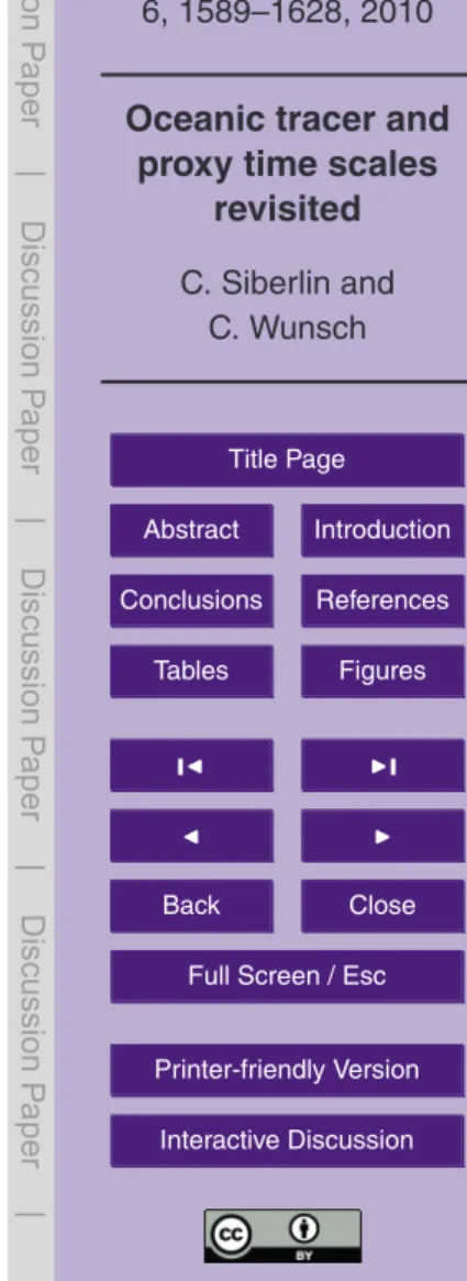
ern Ocean, the dye is upwelled, entering the Antarctic Circumpolar Current (ACC). Then, it advects and diffuses near-bottom into the Pacific and Indian Oceans and there is diffused vertically and upwelled. Figure 3 depicts the concentration at 2000 m after 2000 yr for a concentration-stepC=1 applied in the North Atlantic. Observe that the North Atlantic is at equilibrium (C>90%), the Southern Ocean is atC≈70%,and the

20

Pacific Ocean is atC_≈40% of their final values. The mid-depth Pacific, as expected, takes the longest to reach equilibrium.

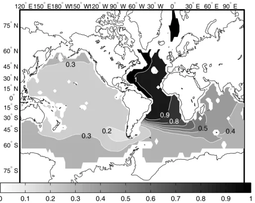
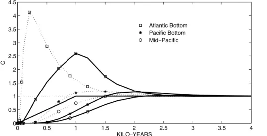
Figure 4 shows the evolution of the dye average concentration in three regions of the ocean from the North Atlantic concentration step. The time-lag of 4000 yr between the bottom of the Atlantic and Pacific is consistent with WH08.

(15)

CPD

6, 1589–1628, 2010

revisited

Title Page

Tables Figures

◭ ◮

Back Close

Full Screen / Esc

Discussion

P

a

per

|

Dis

cussion

P

a

per

|

Discussion

P

a

per

|

Discussio

n

P

a

per

|

3.3 North Pacific Injection

A concentration-step applied in the North Pacific Ocean north of 45◦N provides a useful comparison to the injection of tracer in an area of deep water formation. Here, the dye sinks in the North Pacific and stabilizes near 1000 m. It is advected to the south by the subtropical gyre, crossing the basin zonally to the west, being carried by the North

5

Equatorial Current and driven further to the south into the Indian Ocean through the Indonesian Passages, a route which was also observed by WH08. Carried eastward by the ACC, the dye is moved into the Atlantic Ocean by the surface currents – on the West African coast first – where the model Benguela Current operates, then zonally at the latitude of the South Equatorial current and finally northward in the model Gulf Stream.

10

When reaching the Atlantic northern boundary, it is carried convectively downward and then advected south again within the NADW.

Figure 5 shows the concentration at 2000 m after 2000 yr for concentration-step,

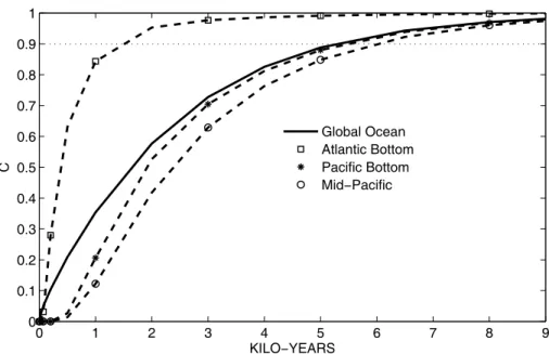
C=1,in the North Pacific region. Even with North Pacific injection, the mid-depth Pa-cific takes the longest time to reach equilibrium, which is again consistent with WH08.

15

Note that in the modern world, there is a significant Arctic Basin flow of order 1 Sv between the North Pacific and the North Atlantic, which could make the times to equi-librium smaller in this critical area – by shortening the time necessary to transfer the dye at the Pacific surface to a region of deep convection (North Atlantic instead of the Circumpolar area; WH08). The present configuration is perhaps more suitable for the

20

Last Glacial Maximum with a closed Bering Strait. Figure 6 shows the evolution of the average dye concentration in three regions from the North Pacific concentration step. All regions remain far from equilibrium after 10 000 yr. The bottom of the tropical At-lantic barely reaches 50% of its final concentration after 7000 yr, with the Pacific further behind (the bottom of the tropical Pacific reaches 50% of its final concentration after

25

(16)

CPD

6, 1589–1628, 2010

revisited

Title Page

Tables Figures

◭ ◮

Back Close

Full Screen / Esc

Discussion

P

a

per

|

Dis

cussion

P

a

per

|

Discussion

P

a

per

|

Discussio

n

P

a

per

|

3.4 Dirichlet and Neumann boundary conditions

The time histories in the North Atlantic and North Pacific are different and depend on the injection region. The paths taken by the dye for the three boundary conditions – concentration-step, flux-step, flux-pulse – are similar, but the time-scales on which the equilibrium is achieved are drastically different.

5

Figures 7 and 8 depict the evolution of concentration in three different regions of the ocean, when a Neumann flux-pulse is imposed in the North Atlantic and the North Pacific for two external time-scales Text: a pulse of 1 yr (Text=1 yr) and of 1000 yr

(Text=1000 yr). The overshoots in concentration beyond C=1 are the consequence

of the initial high concentrations at the surface. For Text=1, t90 is shorter than in the 10

concentration-step experiments. The time lag∆t90(the time difference between the

Pa-cific and Atlantic bottom reaching 90% of its final value) is also shorter than the 4000-yr delay observed in the Dirichlet-Heaviside North Atlantic experiment (as in PD09). Here all the dye has been introduced in the ocean after a year and is then homogenized by advection and diffusion processes. In the Dirichlet experiment however, the

con-15

centration boundary condition prescribed implies a flux between the surface patch and the waters underneath that is time-dependent: the tracer gradient normal to the patch depends on the rate at which waters are moving away from the patch (PD09). This gra-dient will decrease with time, as the ocean is moving toward uniform dye concentration. When theText=1000 yr, t90 and ∆t90 increase as well. Even with a 1000-yr pulse, the 20

resulting concentration at the surface can reachC=200 because the dye accumulating in those areas leads to large interior derivatives, and at least a regional acceleration toward local equilibrium.

These figures make a general, important, point – what appears pulse-like in one part of the ocean is transformed by the fluid physics into a quite different time-dependent

25

(17)

CPD

6, 1589–1628, 2010

revisited

Title Page

Tables Figures

◭ ◮

Back Close

Full Screen / Esc

Discussion

P

a

per

|

Dis

cussion

P

a

per

|

Discussion

P

a

per

|

Discussio

n

P

a

per

|

transients as they move through the advecting and diffusing ocean is both qualitatively and quantitatively important, and interpreting what might be recorded in the sediments can only be done with knowledge of the transformation process. This process will produce differing results depending upon, among other elements, whether injection is local or global. Appendix 2 shows an analytical example of the change from a pulse to

5

a distorted rise in a one-dimensional, purely diffusive system.

3.5 Decaying tracer

The impact of a decay constant on tracer ages has been extensively studied both theoretically and numerically (e.g., Khatiwala et al., 2001, 2007; Waugh et al., 2002, 2003; Gebbie and Huybers, 2010b). “Tracer age” is usually defined as the elapsed

10

time since the tracer was injected into the flow at the sea surface (e.g., Holzer and Hall, 2000) and, as discussed in the Introduction, would be simple to interpret if only a single origination time and place needed to be considered. In a general circulation model, one can calculate the varying components contributing at any given location, and use the resulting fractions to find a true mean age and the full range of contributing

15

arrival times. In observations used alone, as we have seen, the apparent age can be a strongly biassed estimate of the mean age.

Consider a Dirichlet-Heaviside, concentration-step, C=1, applied in the North At-lantic Ocean for a radiocarbon tracer. Those results can directly be compared to the previous North Atlantic stable tracer experiment. Siberlin (2010) studied three different

20

radioactive tracers – 3H (tritium, λ−1=12 yr), 91Nb (λ−1=700 yr), 14C (λ−1=5730 yr) – and computed their concentration evolution and ages. In the case of tritium, the half-life is so small that the tracer decays before reaching the Pacific Ocean. Table 1 dis-playst90 and ages for the three decaying tracers. The moreλ−

1

increases, the longer the equilibrium times and the more the tracer age underestimatest90. Many ages or 25

(18)

CPD

6, 1589–1628, 2010

revisited

Title Page

Tables Figures

◭ ◮

Back Close

Full Screen / Esc

Discussion

P

a

per

|

Dis

cussion

P

a

per

|

Discussion

P

a

per

|

Discussio

n

P

a

per

|

is approximately conventional. This map should be compared to Fig. 10 of WH08 for

t90.Ages are the oldest in the Pacific and the youngest in the Atlantic. On the Pacific

bottom, they are of the order of ∼2500 yr and on the Atlantic bottom ∼500 yr. Those results are pictorially consistent with the mapped deep radiocarbon ages of Matsumoto (2007, his Fig. 1). Because of the biases, their interpretation is not so clear.

5

The issue of the most appropriate idealized boundary condition is not entirely obvi-ous, although the Robin condition (PD09) is the most natural one, subject to choices of the constants.1 Note (e.g., Bard, 1988), that the surface North Atlantic has a radiocar-bon age of about 400 yr, showing that the14C concentration there reflects an exchange with the fluid underneath. A more straightforward problem could be posed by including

10

calculation of the atmospheric concentration as part of the required solution, one in which spatial and temporal variations in upwelling/downwelling and mixing at the base of a time-dependent mixed-layer etc., would be accounted for along with the changing atmospheric concentrations.

4 Some paleoclimate applications 15

Studies based on paleodata such as the ones of Skinner and Shackleton (2005) and Lea et al. (2000), using radiocarbon ages, are two examples of attempts to describe the last deglaciation on a regional scale. Between the Atlantic and Pacific bottom however, we calculate heret90 from 500 to 4000 yr, with a mean value of ∼1300 yr. No

signifi-cant di_fferences are observed between the boundaries and the centers of the abyssal

20

basins. Theδ18O signals retrieved from the Skinner and Shackleton (2005) cores are believed to be consistent records of theδ18O of the deep water at the Iberian margin and the eastern equatorial Pacific. From the present results, the glacio-eustatic signal resulting from deglaciation should appear in the cores witht90differences between the

1

(19)

CPD

6, 1589–1628, 2010

revisited

Title Page

Tables Figures

◭ ◮

Back Close

Full Screen / Esc

Discussion

P

a

per

|

Dis

cussion

P

a

per

|

Discussion

P

a

per

|

Discussio

n

P

a

per

|

Pacific and Atlantic abysses of hundreds to thousands of years.

Furthermore, the temperature of those deep water masses depends essentially on their condition of formation, that is, on the temperature in the area of deep water forma-tion. If we consider sufficiently small changes, temperature is expected to behave as a passive tracer. Therefore, as theδ18O in benthic foraminifera is not uniformly a_ffected

5

by changes in the passive glacio-eustatic signal, it would not be uniformly affected by deep water temperature fluctuations either. Large shifts in temperature will change the flow and cannot be treated as a passive tracer. How equilibrium times are changed can only be understood by carrying out a full calculation.

Another example of the use of time delay information is in the core discussed by Lea

10

et al. (2000) in the eastern tropical Pacific near the Galapagos chain. From a passive tracer flux-pulse applied in the North Atlantic, the time required for the sub-surface (0 to 500 m) disturbance in the eastern equatorial Pacific to reacht90 exceeds 1500 yr

although atmospheric pathways require timescales that are far shorter. The fraction of

δ18O seen near-surface at the Galapagos owing to a water pathway, as opposed to

15

an atmospheric one, is unknown. Lea et al. (2000) infer a lag of approximately 3 kyr between the Mg/Ca (primarily a temperature signal) and the δ18O (primarily an ice volume signal) in the planktonic foraminifera in the core, and interpret that to mean that the sea-surface temperature change in the eastern equatorial Pacific led the ice-sheet melting. Furthermore, Lea et al. (2000) conclude that their eastern equatorial

20

SST record is synchronous with Petit et al. (1999) temperature records in Antarctica “within the 2-kyr resolution of the sites”. But the ice volumeδ18O tracer may have taken several thousand years to reach the core region via the oceanic pathway. Furthermore, in the modern world, high latitude warming is much larger than in the tropics, and one might anticipate that the lower latitude response will be relatively muted, and delayed.

25

(20)

CPD

6, 1589–1628, 2010

revisited

Title Page

Tables Figures

◭ ◮

Back Close

Full Screen / Esc

Discussion

P

a

per

|

Dis

cussion

P

a

per

|

Discussion

P

a

per

|

Discussio

n

P

a

per

|

5 Discussion

The matrix method developed by Khatiwala et al. (2005) permits fast computation of the steady and transient states for passive tracers, in which the results are qualtitatively consistent with those obtained by direct integration of the full underlying GCM. Con-sistent with the results of both WH08 and PD09, the time histories of transient tracers

5

within the ocean have a complex behavior dependent upon the details of the boundary conditions, including not only where and how the tracer is input (Dirichlet, Neumann, or mixed boundary conditions), but also the duration (and area) of a pulse relative to the many internal time scales of tracer movement.

In particular, the time differences required for two oceanic areas to reach a certain

10

concentration depends on those details. If age models in cores are set by matching peaks in the local signals and interpreted as at least a momentary equilibrium, one must also be alert to the differing nature of the transient approach to equilibrium, most apparent e.g., in the Neumann-pulse cases, where the values may be approached from above in the near-injection region. In many cases not specifically addressed here, the

15

surface boundary conditions may well have changed long before equilibrium is reached in the entire ocean. In other cases, time differences of several thousand years may be irrelevant – being indistinguishable in the data.

The information content of tracers is not, of course, limited to a reduction to either “age” or equilibrium times. Spatial and temporal gradients at any given time provide

20

information, or at least bounds, on the different terms in equations such as Eq. (1) and these could prove fruitful, depending upon the errors introduced by terms that cannot be measured. Similarly, multiple tracers, if imposed with known boundary conditions with adequate accuracy in both space and time, can potentially produce useful bound-ing values of various oceanic processes.

(21)

CPD

6, 1589–1628, 2010

revisited

Title Page

Tables Figures

◭ ◮

Back Close

Full Screen / Esc

Discussion

P

a

per

|

Dis

cussion

P

a

per

|

Discussion

P

a

per

|

Discussio

n

P

a

per

|

Boundary conditions

PD09 and F. Primeau and E. Deleersjinder (private communication, 2010) have empha-sized the important influence that the choice of boundary condition can make on the resulting time histories. We do not wish here to over-emphasize the direct relevance of our use of a Dirichlet (concentration) surface boundary condition, but regard it as

5

producing, in the geophysical fluid dynamics sense, possibly the simplest method for delineating the space-time behavior a three-dimensional ocean circulation. Readers need to keep in mind that the evolution of a tracer, and its interpretation does depend both qualitatively and quantitatively on the details of mechanical injection versus dif-fusion, gas exchange, precipitation, as well as the space and time changes that are

10

inevitable, including seasonality, none of which are discussed here.

For real tracers, the nature of the boundary condition also depends on more than the tracer. For example, theδ18O distribution is probably best determined from a flux boundary condition, because the input will be dominated by the melting rate of injected ice, or the net evaporation rate. On the other hand, in a calculation in which the melted

15

ice was initially supposed confined to the mixed layer, the boundary condition most suitable for the ocean below may well be a concentration one, or one represented as the mixed boundary condition – it would depend upon the nature of the surface representation in a particular model.

For paleoclimate studies, the most important inference is that the tracer is far from

20

being instantaneously homogenized with times to near-equilibrium extending for thou-sands of years, and differing sometimes greatly from radiocarbon ages – being uni-formly longer. Ages determined from decaying isotope measurements are biassed to be younger than true mean ages or equilibrium times.

Model limitations 25

(22)

CPD

6, 1589–1628, 2010

revisited

Title Page

Tables Figures

◭ ◮

Back Close

Full Screen / Esc

Discussion

P

a

per

|

Dis

cussion

P

a

per

|

Discussion

P

a

per

|

Discussio

n

P

a

per

|

spatial resolution. The long-term behavior of so-called eddy resolving models of the ocean circulation could be very di_fferent than the coarse resolution ones used in climate studies (see e.g., Hecht and Smith; 2008; L ´evy et al., 2010).

In this model configuration, no “real” ice is formed. The increase of surface water density is the consequence of the low winter temperatures only. Input of freshwater

5

from melting ice at the edges is not represented, nor is the physics of the complex mixed-layer known to be present. When using a 1◦ horizontal resolution, 21-vertical layer configuration of the MITgcm Marshall et al. (1997) as modified in ECCO-GODAE, WH08, note some evidence that the model has too-active convection in the North At-lantic, and which will artificially shorten tracer movement times. On the other hand,

10

when tracer injections occur in regions of AABW formation, we are most likely overes-timating the equilibrium times (and those experiments are not described here). Pro-duction of AABW depends upon small scale processes taking place on the continen-tal margin and involving complex topography, ice shelves, sea ice, and details of the equation-of -state. As a result, the AABW formation is not correctly represented in the

15

model, with the North Atlantic region dominating the dye concentration of the deep-est model layers (WH08). Coarse resolution also prevents an adequate representation of major surface current systems such as the Gulf Stream. Parameterization of the higher resolution features, such as eddies, prevents accurate transport of the dye, es-pecially on the boundaries. With higher resolution, the model would produce higher

20

speed flows and the dye would be advected faster from one point of the ocean to the other. On the other hand, higher resolution also weakens the implicit diffusion exist-ing through the advection scheme, and which would slow the approach to equilibrium. Even if seasonal cycles are present in the underlying GCM code, the use of annual averages of the transition matrices also affects the results. In addition, the vertical

25

(23)

CPD

6, 1589–1628, 2010

revisited

Title Page

Tables Figures

◭ ◮

Back Close

Full Screen / Esc

Discussion

P

a

per

|

Dis

cussion

P

a

per

|

Discussion

P

a

per

|

Discussio

n

P

a

per

|

Active tracers

Apart from the problem of model resolution, probably the greatest limitation on the present study is its restriction to passive tracers – those not affecting the density field – because a state-transition matrix method is not yet available for the situation where the flow field is changed by the tracer. Although tracers such asδ18O are themselves

5

passive, they are commonly associated with anomalous temperature or salinities in the water carrying them, and hence they are part of an active response. Whether a simple generalization can be made – that active processes will shorten or lengthen the passive tracer response times – is not clear at the moment. Anomalous density fields can increase (decrease) active pressure gradients and hence flows, but they are

10

also subject to confinement by strong rotational constraints, thus slowing the response. Preliminary results for an active tracer using direct integration of a 2◦-grid resolution global circulation model limited to the North Atlantic box (Siberlin, 2010) show no sig-nificant differences between a small injection of freshwater (0.001 Sverdrups) and of passive dye within the first 50 yr of the experiments: the pathways as well as the times

15

required for a change in salinity versus dye concentration are similar. However, any small differences in this critical period could lead to strong differences in the far future as pathways diverge with time. The modern ocean is also different from the oceans of the past. At some future time, it will be worthwhile attempting a more detailed estimate of the paleocean circulation.

20

Final remarks

In the interim, lead-lag times of apparent shifts in climate record features shorter than about 5000 yr need to be viewed cautiously. Radiocarbon ages are particularly prob-lematic when used for causality inferences because of their bias toward younger times. Aside from the usual age-model uncertainties, the ocean all by itself is capable of

25

(24)

CPD

6, 1589–1628, 2010

revisited

Title Page

Tables Figures

◭ ◮

Back Close

Full Screen / Esc

Discussion

P

a

per

|

Dis

cussion

P

a

per

|

Discussion

P

a

per

|

Discussio

n

P

a

per

|

the result of fully three-dimensional processes. Thus the signal propagation from e.g., the surface North Pacific to the abyssal or intermediate depth North Pacific, is a long and circuitous route not immediately related to the apparently short vertical distance involved. At the present time, for these lead-lag times, there appears to be little alter-native except to carry out model integrations through the circulation that are as realistic

5

as possible. Even though the details are unlikely to survive further developments, the gross propagation times and degree of pulse shifts should prove robust features of the circulation.

Appendix A 10

Model configuration

The model and boundary conditions

Surface temperature and salinity are weakly restored to a climatology (Levitus et al., 1998). The configuration uses a third-order direct space time advection scheme (“DST3”, linear) with operator splitting for tracers, and a variety of parameterizations to

15

represent unresolved processes, including the Gent and McWilliams (1990) eddy-flux parameterization and the Large et al. (1994) mixed layer formulation (or “KPP”).Aeand

Ai (the explicit and implicit transport matrices) are derived at monthly resolution from

the equilibrium state of the model after 5000 yr of integration (Khatiwala, 2007). In some sub-region,B1,whose area is all, or a fraction, ofB,the boundary condition 20

on C is imposed. WH08 carried out a series of experiments in which the so-called ECCO-GODAE solution v2.216 was used in a perpetual 14-yr loop, specifying both

v and K. v was determined from a least-squares fit of the GCM to a modern data base consisting of over 2×109 observations, and thus was believed to be realistic up to the various model approximations (of which the 1◦ spatial resolution is believed to

25

(25)

CPD

6, 1589–1628, 2010

revisited

Title Page

Tables Figures

◭ ◮

Back Close

Full Screen / Esc

Discussion

P

a

per

|

Dis

cussion

P

a

per

|

Discussion

P

a

per

|

Discussio

n

P

a

per

|

conditions onC, WH08 imposed

Cbd y(r∈B1,t)=1H(t), (1a)

∂C_{bd y}(r6∈B1,t)

∂z =0 (1b)

where H(t) is the Heaviside function, H(t)=0, t<0; H(t)=1, t≥1. r is a

three-5

dimensional position vector. Or, in words, att=0,the concentration at the sea surface in the sub-regionB1 was abruptly set to unity, and maintained at that value ever after.

Outside the subregion (if any), the flux into or out of the ocean was set to zero. This particular choice of boundary conditions was made because it permits one to infer the final, asymptotic steady state:C(r,t→ ∞)=1.

10

Appendix B

Pulse distortion

Diffusion distortion

The simplest system with diffusion is the one-dimensional equation,

15

∂C ∂t =K

∂2C ∂z2,

with the intitialC(z,t=0)=0.At the top boundary,C₀(t)=δ(t), a pure pulse. The solution to the above equation is then the boundary Green function

G(z,t)=_√1

π

e−z2/4t

√

(26)

CPD

6, 1589–1628, 2010

revisited

Title Page

Tables Figures

◭ ◮

Back Close

Full Screen / Esc

Discussion

P

a

per

|

Dis

cussion

P

a

per

|

Discussion

P

a

per

|

Discussio

n

P

a

per

|

in distance units ofL, and time units of L2/K. The result for several values of −z is shown in Fig. 11. A “core” recording the time change atz=1,might lead one to infer that the same event did not occur atz=5. This one-dimensional example mimics the gross behavior of the change in behavior seen over large distances in the GCM results.

Acknowledgements. Supported in part by the National Science Foundation Grant OCE-5

0824783 and NASA Award NNX08 AF09G. The advice and help of S. Khatiwala and of P. He-imbach were essential to this study. P. Huybers, J. Gebbie, S. Khatiwala, F. Primeau and E. Deleersnijder made several very useful suggestions.

References

Bard, E.: Correction of accelerator mass spectrometry 14C ages measured in planktonic 10

foraminifera: paleoceanographic implications, Paleoceanography, 3, 635–645, 1988. Brogan, W.: Modern Control Theory. Third Ed., Prentice-Hall, Englewood Cliffs, NJ, 1991. Gebbie, G. and Huybers, P.: How is the ocean filled?, Nature, submitted, 2010a.

Gebbie, G. and Huybers, P.: What is the mean age of the ocean? Accounting for mixing histories in the interpretation of radiocarbon observations, J. Phys. Oc., unpublished ms., 15

2010b.

Gent, P. R. and Mcwilliams, J. C.: Isopycnal mixing in ocean circulation models, J. Phys. Oceanogr., 20, 150–155, 1990.

Hecht, M. W. and Smith,. R. D.: Towards a physical understanding of the North Atlantic: a review of model studies, in: Ocean Modeling in an Eddying Regime, edited by: Hecht, M. W. and 20

Hasumi, H., AGU Geophysical Monograph, 177, 213–240, 2008.

Holzer, M. and Hall, T. M.: Transit-time and tracer-age distributions in geophysical flows, J. Atmos. Sci., 57, 3539–3558, 2000.

Khatiwala, S., Visbeck, M., and Schlosser, P.: Age tracers in an ocean GCM, Deep-Sea Res. Pt. I, 48, 1423–1441, 2001.

25

Khatiwala, S., Visbeck, M., and Cane, M. A.: Accelerated simulation of passive tracers in ocean circulation models, Ocean Model., 9, 51–69, doi:10.1016/j.ocemod.2004.04.002, 2005. Khatiwala, S.: A computational framework for simulation of biogeochemical tracers in the

(27)

CPD

6, 1589–1628, 2010

revisited

Title Page

Tables Figures

◭ ◮

Back Close

Full Screen / Esc

Discussion

P

a

per

|

Dis

cussion

P

a

per

|

Discussion

P

a

per

|

Discussio

n

P

a

per

|

Large, W. G., Mcwilliams, J. C., and Doney, S. C.: Oceanic vertical Mixing – a review and a model with a nonlocal boundary-layer parameterization, Rev. Geophys., 32, 363–403, 1994.

Lea, D. W., Pak, D. K., and Spero, H. J.: Climate impact of late Quaternary Equatorial Pacific sea surface temperature variations, Science, 289, 1719–1724, 2000.

5

Ledwell, J. R., Watson, A. J., and Law, C. S.: Evidence for slow mixing across the pycnocline from an open-ocean tracer-release experiment, Nature, 364, 701–703, 1993.

Levitus, S., Boyer, T. P., Conkright, M. E., et al.: World Ocean Database 1998. NOAA Atlas NESDIS 18, NOAA, Silver Spring MD, 346 pp., 1998.

L ´evy, M., Klein, P., Treguier, A. M., Iovino, D., Madec, G., Masson, S., and Takahashi, K.: 10

Modifications of gyre circulation by sub-mesoscale physics, Ocean Model., 34, 1–15, doi:10.1016/j.ocemod.2010.04.001, 2010.

Marshall, J., Adcroft, A., Hill, C., Perelman, L., and Heisey, C.: A finite-volume, incompress-ible Navier Stokes model for studies of the ocean on parallel computers, J. Geophys. Res.-Oceans, 102, 5753–5766, 1997.

15

Matsumoto, K.: Radiocarbon-based circulation age of the world oceans, J. Geophys. Res.-Oceans, 112, C09004, doi:10.1029/2007jc004095, 2007.

Petit, J. R., Jouzel, J., Raynaud, D., Barkov, N. I., Barnola, J. M., Basile, I., Bender, M., Chappel-laz, J., Davis, M., Delaygue, G., Delmotte, M., Kotlyakov, V. M., Legrand, M., Lipenkov, V. Y., Lorius, C., Pepin, L., Ritz, C., Saltzman, E., and Stievenard, M.: Climate and atmospheric 20

history of the past 420 000 yr from the Vostok ice core, Antarctica, Nature, 399, 429–436, 1999.

Primeau, F. and Deleersnijder, E.: On the time to tracer equilibrium in the global ocean, Ocean Sci., 5, 13–28, doi:10.5194/os-5-13-2009, 2009.

Siberlin, C. and Wunsch, C.: Time-Scales of Passive Tracers in the Ocean with Paleoapplica-25

tions, Master’s thesis, Massachusetts Institute of Technology, 134 pp., 2010.

Skinner, L. C. and Shackleton, N. J.: An Atlantic lead over Pacific deep-water change across Termination I: implications for the application of the marine isotope stage stratigraphy, Qua-ternary Sci. Rev., 24, 571–580, doi:10.1016/j.quascirev.2004.11.008, 2005.

Waugh, D. W., Vollmer, M. K., Weiss, R. F., Haine, T. W. N., and Hall, T. M.: Transit time 30

distributions in Lake Issyk-Kul, Geophys. Res. Lett., 29, 2231, doi:10.1029/2002gl016201, 2002.