Observations of I<sub>2</sub> at a remote marine site

(1)

ACPD

13, 25911–25937, 2013

I2in the MBL M. J. Lawler et al.

Title Page

Abstract Introduction

Conclusions References

Tables Figures

◭ ◮

Back Close

Full Screen / Esc

Printer-friendly Version

Interactive Discussion

Discussion

P

a

per

|

D

iscussion

P

a

per

|

Discussion

P

a

per

|

Discuss

ion

P

a

per

|

Atmos. Chem. Phys. Discuss., 13, 25911–25937, 2013 www.atmos-chem-phys-discuss.net/13/25911/2013/ doi:10.5194/acpd-13-25911-2013

Atmospheric Chemistry and Physics

Open Access

Discussions

This discussion paper is/has been under review for the journal Atmospheric Chemistry and Physics (ACP). Please refer to the corresponding final paper in ACP if available.

Observations of I

₂

at a remote marine site

M. J. Lawler1,*, A. S. Mahajan2,**, A. Saiz-Lopez2, and E. S. Saltzman1

1

Department of Earth System Science, University of California, Irvine, USA 2

Atmospheric Chemistry and Climate Group, Institute of Physical Chemistry Rocasolano, CSIC, Madrid, Spain

*

currently at: Department of Environmental Physics, University of Eastern Finland, Kuopio, Finland; visitor at National Center for Atmospheric Research, Boulder, USA

**

currently at: Indian Institute of Tropical Meteorology, Pune, India

Received: 20 August 2013 – Accepted: 3 September 2013 – Published: 9 October 2013

Correspondence to: M. J. Lawler (mlawler@ucar.edu)

(2)

ACPD

13, 25911–25937, 2013

Title Page

Tables Figures

◭ ◮

Back Close

Full Screen / Esc

Discussion

P

a

per

|

D

iscussion

P

a

per

|

Discussion

P

a

per

|

Discuss

ion

P

a

per

Abstract

Inorganic iodine plays a significant role in the photochemistry of the marine bound-ary layer, but the sources and cycling of iodine are not well understood. We report the first I₂observations in marine air that is not impacted by coastal macroalgal emis-sions or sea ice chemistry. The data clearly demonstrate that the very high I2 levels

5

previously reported for coastal air are not representative of open ocean conditions. In this study, gas phase I₂was measured at the Cape Verde Atmospheric Observatory, a semi-remote site in the eastern tropical Atlantic, using atmospheric pressure chemical ionization tandem mass spectrometry. Atmospheric I2levels typically increased

begin-ning at sunset, leveled offafter midnight, and then rapidly decreased at sunrise. There 10

was also a smaller midday maximum in I2that was at least partly due to a measurement

artifact. Ambient I2 mixing ratios ranged from<0.02–0.6 pmol mol− 1

in May 2007 and

<0.03–1.67 pmol mol−1in May 2009. The sea-air flux implied by the nighttime buildup

of I₂is too small to explain the observed daytime IO levels at this site. Iodocarbon mea-surements made in this region previously are also insufficient to explain the observed 15

1–2 pmol mol−1 of daytime IO. The observations imply the existence of an unknown daytime source of gas phase inorganic iodine. Carpenter et al. (2013) recently pro-posed that sea surface emissions of HOI are several times larger than the flux of I2.

Such a flux could account for both the nighttime I2and the daytime IO observations.

1 Introduction

20

Iodine in the marine atmosphere is ultimately derived from the iodide, iodate, and or-ganically bound iodine contained in seawater. Iodine emitted from the sea surface un-dergoes rapid photochemical transformations involving both gas phase and heteroge-neous reactions (Vogt et al., 1999; von Glasow, 2003; Saiz-Lopez et al., 2008). Iodine chemistry can potentially influence climate through the catalytic destruction of tropo-25

(3)

mag-ACPD

13, 25911–25937, 2013

Title Page

Tables Figures

◭ ◮

Back Close

Full Screen / Esc

Discussion

P

a

per

|

D

iscussion

P

a

per

|

Discussion

P

a

per

|

Discuss

ion

P

a

per

|

nitudes of these processes are not fully understood. Marine iodine chemistry also im-pacts human health. The emissions, atmospheric transport, and deposition of marine iodine to the land surface influences the availability of this essential nutrient (Johnson, 2003, and references therein). Reactive forms of inorganic iodine may contribute to the conversion of elemental mercury to bioavailable oxidized states, posing a hazard to 5

human and ecosystem health (Saiz-Lopez et al., 2008; Raofie et al., 2008).

Iodine can be emitted from the sea surface in several different forms. It has been known for some time that O3 deposited to the sea surface can react with I− in the

surface seawater to release I2. Rates of I2 release from this process have been

es-timated at around 2×106molec cm−2s−1, or 2.9 nmol m−2d−1 (Garland and Curtis, 10

1981). More recent laboratory and modeling work has considered the release of HOI from this process as well, yielding estimates of daytime fluxes of 100 nmol m−2d−1and 10 nmol m−2d−1 for HOI and I2, respectively (Carpenter et al., 2013). That represents

an increase of roughly 20x the per-I-atom flux relative to what was previously thought . Because I− is ubiquitous in the surface ocean, this process must occur globally and 15

could account for a flux of elemental I on the order of 2 Tg yr−1. Certain species of coastal macroalgae directly emit copious quantities of I₂, particularly while under ox-idative stress (Saiz-Lopez and Plane, 2004; Dixneuf et al., 2009; McFiggans et al., 2004; Palmer et al., 2005). In the open ocean, planktonic algae may also release I2, but

the open ocean emission rate is not known (Amachi et al., 2000; Jones et al., 2010). 20

Organoiodide compounds such as CH2I2 and CHClI2 are also emitted from the sea

surface. Like I2, most of these compounds are rapidly photolyzed, releasing I atoms

on timescales of minutes in the daytime marine boundary layer. The most abundant and longest-lived organoiodide compound, methyl iodide, has a photolysis lifetime of several days. The global I release attributed to organoiodides is on the order of 0.4– 25

1 Tg I yr−1, with CH₃I dominating (Jones et al., 2010, and references therein).

Once formed in air, iodine atoms can initiate catalytic ozone destruction cycles such as those below:

(4)

ACPD

13, 25911–25937, 2013

Title Page

Tables Figures

◭ ◮

Back Close

Full Screen / Esc

Discussion

P

a

per

|

D

iscussion

P

a

per

|

Discussion

P

a

per

|

Discuss

ion

P

a

per

IO+HO2→HOI+O2 (R2)

HOI+hν_→I+OH (R3)

Net: 5

O3+HO2+hν→2O2+OH (R4)

Catalytic destruction of tropospheric ozone by iodine is efficient in part because io-dine radicals are relatively unreactive with organic trace gases.

Sea salt aerosols are thought to play a role in Ix cycling in marine air. I− present in aerosols can be oxidized to the volatile forms ICl, IBr, and I2 via reaction with the

10

hypohalous acids HOCl, HOBr, or HOI. The hypohalous acids are generated by gas phase daytime photochemistry (e.g. Reactions 1–2) and can enter aerosols to react with I−:

HOI+I−₊_H+_→_I

2+H2O (R5)

Iodine radicals can also self-react to form iodine oxides such as I2O4and other larger

15

iodine oxide clusters (McFiggans et al., 2004; Saiz-Lopez et al., 2006). If iodine levels are sufficiently high, the formation of iodine oxides leads to rapid particle nucleation. IOx-driven nucleation events have been observed downwind of I2-emitting macroalgae

beds. These events contribute to aerosol number and can potentially influence cloud properties in coastal regions (Saunders et al., 2010; Mahajan et al., 2010).

20

(5)

ACPD

13, 25911–25937, 2013

Title Page

Tables Figures

◭ ◮

Back Close

Full Screen / Esc

Discussion

P

a

per

|

D

iscussion

P

a

per

|

Discussion

P

a

per

|

Discuss

ion

P

a

per

|

destruction (Read et al., 2008). The source of reactive iodine at CVAO remains an open question. Jones et al. (2010) measured air-sea dihalomethane fluxes in open ocean and upwelling Atlantic waters near Cape Verde. They observed iodocarbons in these waters at levels too low to account for the observed IO at CVAO and proposed that a large I2 flux might account for the discrepancy. Using a 0-D box, model, they

5

incorporated a constant I2flux large enough to achieve the IO levels observed at Cape

Verde. This resulted in nighttime I2levels of up to 7 pmol mol− 1

. Mahajan et al. (2010) used the same observations and a vertically resolved model with an I₂ source which was allowed to vary. They concluded that an additional MBL source of I2 may be

re-quired to explain the observed IO levels, but that the source may have a strong diel 10

cycle (Mahajan et al., 2010). Mahajan et al. (2012) observed slant column IO densities corresponding to roughly 1 pmol mol−1during shipboard measurements in the eastern Pacific.

In this manuscript we report nighttime levels of gas phase I₂ at Cape Verde during measurement campaigns over three weeks in May–June 2007 and one week in May 15

2009. The only other reported observations of I2in marine air have been conducted in

regions influenced by emissions from coastal macroalgae or by I₂production on sea ice surfaces (Saiz-Lopez et al., 2012; Atkinson et al., 2012). These observations provide estimates of I2levels and production rates that are more representative of open ocean

conditions than previous studies. 20

2 Study site and observational methods

2.1 Setting and ancillary observations

The field site was the Cape Verde Atmospheric Observatory (CVAO), located at 16.864◦N, 24.867◦W on the island of São Vicente. The site is situated about 50 m from a northeast facing coastline, about 10 m above sea level. The island is volcanic in ori-25

(6)

ACPD

13, 25911–25937, 2013

Title Page

Tables Figures

◭ ◮

Back Close

Full Screen / Esc

Discussion

P

a

per

|

D

iscussion

P

a

per

|

Discussion

P

a

per

|

Discuss

ion

P

a

per

two study years, 2007 and 2009. Winds were consistently onshore during both years, and 15 min averaged windspeeds were 7.67±1.47 m s−1 (1 std dev) with a 3.6–10.4 range in 2009 and 6.17±1.35 (2.2–8.7 range) in 2007. See Carpenter et al. (2011) for a thorough site overview. NOx (NO +NO2) was measured by chemiluminescence at

a height of 3 m above the ground. The instrument had a detection limit of<14 ppt for

5

reported 15 min means. NOxlevels were typically below 25 ppt in 2007, without a

dis-cernible diel pattern. In 2009 the daytime NOxlevels were higher and had a distinct diel

cycle, with a typical midday NO2maximum of 40–50 pmol mol− 1

and a late afternoon NO maximum of about 15 pmol mol−1. The 2009 NO_x measurements may have been influenced by the site diesel generator. The generator was located about 100 m away 10

from the site in 2007, but it was moved directly adjacent to the downwind side of the site in 2009. O₃was measured at 3 m by UV absorption. O₃was 33.4±5.3 nmol mol−1 in 2007 and 36.2±5.0 nmol mol−1in 2009 (mean±1 std. dev.). Lee et al. (2010) give an overview of NOxand O3observations at the site.

2.2 I2detection by chemical ionization mass spectrometry

15

I₂ detection was carried out by chemical ionization triple quadrupole mass spectrom-etry using a modified Thermo TSQ Quantum instrument, with procedures similar to those in previously published studies of Cl2, Br2, and I2(Lawler et al., 2009; Finley and

Saltzman, 2008). The mass spectrometer was fitted with a63Ni beta-emitting source, and ambient I₂molecules were ionized to I−

2. The I −

2 ions were mass-selected in the first

20

quadrupole (Q1), then dissociated by collision with Ar in Q2 (20 eV) to form I−, which was in turn mass selected (Q3) and detected by a electron multiplier after impaction on a dynode. Mass transitions for ICl− →Cl− and IBr−→Br−were also monitored.

The instrument background signal was assessed every hour by sampling ambient air which was scrubbed of I2. The scrubber was a carbonate-coated plug of glass

25

(7)

ACPD

13, 25911–25937, 2013

Title Page

Tables Figures

◭ ◮

Back Close

Full Screen / Esc

Discussion

P

a

per

|

D

iscussion

P

a

per

|

Discussion

P

a

per

|

Discuss

ion

P

a

per

|

efficiency (∼99 %) when fresh but degrades after a few weeks of use. There was no evidence that the scrubber degraded over the campaign.

An I2 gas standard was generated by flowing N2 over an I2 permeation tube in a

temperature-controlled PFA housing. This I₂/N₂flow was subsampled and diluted with additional N₂ to a final sampled mixing ratio of 2–16 pmol mol−1 _{in the method of}

Gal-5

lagher et al. (1997). I2 in the dilution system was only exposed to PFA and PTFE

surfaces. The standard gas flowed continuously through a length of PFA tubing up to a pneumatic PTFE valve near the top of the inlet. The valve was kept near the inlet to min-imize equilibration time in the tubing. The outdoor tubing was shielded from radiation by opaque insulation to prevent photolysis of the standard I2. During regular ambient

10

sampling intervals, the I₂standard was routed to a container of scrubber material. The output of the I2 permeation tube was gravimetrically calibrated in the laboratory after

the campaign. There were no standards for ICl or IBr.

Instrument sensitivity for I₂ was assessed by performing multipoint calibrations and one-point standard additions. Sensitivity was assumed to vary linearly between cali-15

brations and standard additions. In both 2007 and 2009, the one-point I2 standards

were added on a 4 h schedule on every third day of measurements. Multipoint calibra-tions were run less frequently but consistently showed linear instrument response in the range of observed I2. For these calibrations and single point standards, I2 in N2

was added near the front of the inlet. 20

2.3 Sample inlets

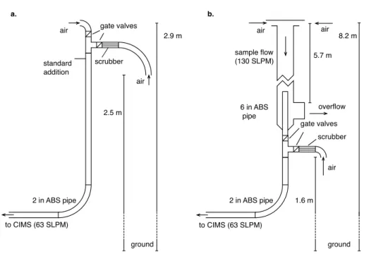
The air sampling inlet used in 2007 is the same as that described previously for Cl2

observations made at this site (Lawler et al., 2009). The setup is illustrated in Figure 1. Ambient air was drawn through a nominal 2 in (5.1 cm) acrylonitrile-butadiene-styrene (ABS) pipe from a height of 3 m. The flow in this pipe was dynamically controlled at 63 25

(8)

ACPD

13, 25911–25937, 2013

Title Page

Tables Figures

◭ ◮

Back Close

Full Screen / Esc

Discussion

P

a

per

|

D

iscussion

P

a

per

|

Discussion

P

a

per

|

Discuss

ion

P

a

per

A longer inlet was used for the 2009 study. Air was drawn from a height of 8 m above the ground into a nominal 6 in (15.24 cm ID) ABS sample pipe at 130 LPM (STP). This flow was controlled using a differential pressure flow sensor, butterfly valve, and PID controller (Omega Engineering, MKS instruments). The flow measurement was calibrated against a mass flow meter (TSI) at the end of the measurements. A 63 LPM 5

subsample was drawn from the center of the main flow through a coaxial nominal 2 in (5.1 cm ID) ABS pipe, with the mass flow control system used in the 2007 deployment. The mass spectrometer sampled 1.3 LPM from the center of the 2 in pipe. During 2009, scrubbed air was introduced directly into the 2 in pipe at the base of the large 8 m inlet (Fig. 1).

10

There were minor di_fferences in the standardization procedure between the two stud-ies. I2 gas standards were added in scrubbed air in 2007, and in ambient air in 2009.

No significant difference in sensitivity has been found for scrubbed vs. unscrubbed air. The sensitivity was assumed to vary linearly between one-point standards, except for obvious step changes in sensitivity.

15

3 Results

3.1 May–June 2007

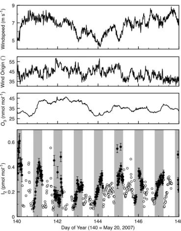
Measured I₂ ranged from <0.02–0.6 pmol mol−1 with a regular diel pattern (Fig. 2).

I2 climbed over the course of the night and reached its highest values either shortly

before dawn or a couple of hours before. I2levels always dropped dramatically at dawn,

20

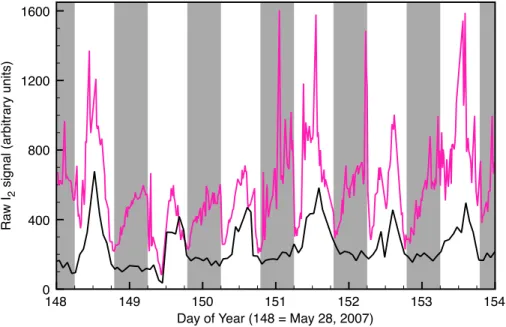
but usually remained at detachable levels. Surprisingly, I₂ levels increased during the daytime, reaching a peak around midday and then declining again before nighttime. I2 levels did not covary with O3 levels. The daytime ’blank’ I2 signals (scrubbed air)

showed large I₂ signals that closely tracked the daytime I₂ increase, but blanks were consistently low and fairly constant over the night (Fig. 4).

(9)

ACPD

13, 25911–25937, 2013

Title Page

Tables Figures

◭ ◮

Back Close

Full Screen / Esc

Discussion

P

a

per

|

D

iscussion

P

a

per

|

Discussion

P

a

per

|

Discuss

ion

P

a

per

|

The ICl sample and blank signals showed similar diel cycles and were statistically indistinguishable from one another. The two ICl mass transitions observed (162→35 and 164→ 37) had a sample signal ratio close to 1, rather than the 3 ratio expected for the two chlorine isotopes. These observations indicate that ICl was not the domi-nant species observed at these transitions. The sample and blank signals for IBr also 5

matched one another, and IBr remained below detection. The actual detection limits for ICl and IBr were not assessed, but detection limits for Cl₂, BrCl, Br₂, and I₂for this instrument are in the range of 0.1–2 pmol mol−1_{, and ICl and IBr detection limits are}

also expected to be in this range.

3.2 May 2009

10

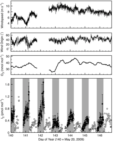
The 2009 I2 levels were very similar to those in 2007, ranging from <0.03–

1.67 pmol mol−1 _{over one week of observations (Fig. 3). The diurnal pattern was also}

very similar, with a nighttime maximum and a smaller daytime peak. There was some day-to-day variability in the absolute levels, with the highest levels occurring late in the night on days 141 and 142. Late on day 141 there was a sudden reduction in wind-15

speed and shift to more northerly flow. Unfortunately the meteorological instruments were not operating on day 142, when the very highest I2levels were measured. There

was some difference in the instrument response to scrubbed air between the two de-ployments. In the 2009 deployment, I2blank signals remained low throughout the day,

and did not exhibit the daytime peak observed in the ambient measurements. 20

3.3 Macroalgal emissions

This is the first study to examine the behaviour of atmospheric I₂in an environment not impacted by iodine-emitting macroalgae. To confirm this, macroalgae were collected from near-site tidal pools and held before the instrument inlet in 2007. No enhancement in I₂ levels was observed for any of the few species found. A container of coastal 25

(10)

ACPD

13, 25911–25937, 2013

Title Page

Tables Figures

◭ ◮

Back Close

Full Screen / Esc

Discussion

P

a

per

|

D

iscussion

P

a

per

|

Discussion

P

a

per

|

Discuss

ion

P

a

per

These observations suggest that the I₂ levels observed are representative of regional oceanic emissions and not influenced by strong local upwind coastal sources.

4 Discussion

4.1 Nighttime I2emission rates

At night, I2 mixing ratios increase steadily after dusk, then level off around midnight

5

(Fig. 5). This suggests I₂emissions that are relatively constant during the buildup, and negligible later in the night. The Cape Verde observations indicate an average nighttime increase of about 0.17 pmol mol−1. Assuming the sea surface is the source and that there are no atmospheric losses, this is a rate of roughly 0.5 pmol mol−1 _d−1 _{over the}

period of constant increase. This corresponds to a sea-to-air flux of 30 nmol m−2d−1, 10

assuming that emissions are diluted into a 1000 m boundary layer and there are no losses. This is about three times the rate estimated in the Carpenter et al. (2013) study.

4.2 I2as a source for daytime IO

Midday maximum IO levels ranging from 1–2 pmol mol−1 were observed by long path DOAS at the CVAO site during May 2007 (Read et al., 2008). Mahajan et al. (2010) 15

and Jones et al. (2010) proposed sea surface emissions of I₂as the principal source of iodine at Cape Verde because air/sea fluxes of organoiodide compounds in the eastern tropical Atlantic were considerably lower than required to account for the observed IO. Model simulations showed that a constant I₂ flux of 170–320 nmol I₂ m−2 _d−1 _was

needed to explain the observed IO (Jones et al., 2010). However, this scenario also led 20

to a nighttime maximum of approximately 7 pmol mol−1of I2and a resultant spike in IO

(11)

ACPD

13, 25911–25937, 2013

Title Page

Tables Figures

◭ ◮

Back Close

Full Screen / Esc

Discussion

P

a

per

|

D

iscussion

P

a

per

|

Discussion

P

a

per

|

Discuss

ion

P

a

per

|

varied with solar flux, from zero at night to a midday maximum of 800 nmol I2m− 2

d−1. That scenario yields nighttime I2 and daytime IO levels that are more consistent with

observations.

4.3 Observations of daytime I2: positive artifact

Midday I2 levels of 0.2 pmol mol− 1

are much larger than would be predicted by the 5

nocturnal emission rate. The noon photolytic lifetime of I2 under CVAO conditions is

roughly 5 s. An I₂ flux large enough to support these levels would result in higher IO levels than observed (see Modeling section below). These considerations, and the fact that the daytime blank I2signals closely tracked the ambient signals in the 2007 study

(see Results section) lead us to conclude that the daytime measurements were a_ffected 10

by a positive experimental artifact.

We hypothesize that the daytime I2 is generated via heterogeneous reactions of a

photochemically produced oxidant with I− _{on the walls of the instrument inlet. This}

would require the oxidant to have the following characteristics; (1) to occur at levels of several pmol mol−1 (or greater), comparable to the measured I2, (2) to be present

15

at significant levels only during daytime, and (3) to be transmitted at least partially through the carbonate scrubber. The first consideration eliminates OH and the second eliminates O3 as likely candidates. The hypohalous acids HOI, HOBr, and HOCl are

photochemically generated daytime oxidants that are present in air at pmol mol−1

lev-els, and are capable of oxidizing I−. HOI can produce I2 directly upon reaction with I−

20

in solution, e.g. (Allen and Keefer, 1955; Vogt et al., 1999). HOBr and HOCl might be expected to initially form IBr and ICl from reaction with I−_{, and further reaction would}

be required to form I2. However, the mixed halogens were not observed in this study.

Previous studies have observed the production of Br2from HOBr and HOCl even on

rel-atively clean inlets, apparently without formation of BrCl (Neuman et al., 2010; Lawler 25

et al., 2011). Analogously, inlet I2production without concomitant ICl or IBr production

(12)

ACPD

13, 25911–25937, 2013

Title Page

Tables Figures

◭ ◮

Back Close

Full Screen / Esc

Discussion

P

a

per

|

D

iscussion

P

a

per

|

Discussion

P

a

per

|

Discuss

ion

P

a

per

The difference in behaviour of the daytime blanks between the two deployments is likely due to the changes in inlet configuration. In 2007, scrubbed air was exposed to the same 3 m long, 2 in ID flow path as the ambient air so the walls of the pipe were coated with ambient aerosols. In this configuration, daytime blanks covaried with the ambient I2 signal. In 2009, scrubbed air was exposed only to the last portion of

5

the inlet, not to the large 6m long 6 ID pipe. In this configuration, the daytime blanks remained low. We speculate that this is because ambient aerosols were deposited near the turbulent sample inlet region of the large pipe, and the scrubbed air encountered only the relatively clean last stage of the inlet.

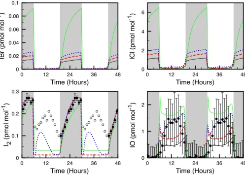
5 Modeling

10

Four model simulations (BASE, FLAT, PHOTO, and HOI, as defined below) were con-ducted to investigate the possible sources of reactive iodine at Cape Verde, given the constraints of observed daytime IO and nighttime I₂ (Fig. 6). The one-dimensional chemical transport model THAMO was used for these simulations (Saiz-Lopez et al., 2008). The model includes gas phase reactive halogen, HOx, NOx, and hydrocarbon

15

chemistry, including a module treating ultrafine particle formation by coagulation of io-dine oxides. It also accounts for recycling of reactive halogens through marine aerosols. In the past, this model has been used to study IO, HOx, and HCHO observations at

Cape Verde (Mahajan et al., 2010, 2011). The model reaction scheme and structure have been described in detail previously (Mahajan et al., 2010; Saiz-Lopez et al., 2008). 20

For all the simulations, the model was constrained with observations of O3(Carpenter

et al., 2011; Lee et al., 2010), HOx (Whalley et al., 2010), NOx(Lee et al., 2009), CH4

and HCHO (Mahajan et al., 2011), and NMHCs (Read et al., 2009) from CVAO. The vertical mixing was calculated using the measured wind speed (Carpenter et al., 2010), using a description detailed by Saiz-Lopez et al. (2008). The model was allowed to run 25

(13)

ACPD

13, 25911–25937, 2013

Title Page

Tables Figures

◭ ◮

Back Close

Full Screen / Esc

Discussion

P

a

per

|

D

iscussion

P

a

per

|

Discussion

P

a

per

|

Discuss

ion

P

a

per

|

In the BASE simulation, standard model chemistry was employed and average sea-air fluxes of halocarbons measured by Jones et al. (2010) near the Cape Verde site were included: CH2I2(13.0 nmol m

2

d−1), CH2IBr (10.9 nmol m 2

d−1), CH2ICl

(16.2 nmol m2d−1d), CH3I (48.5 nmol m 2

d−1), C2H5I (4.1 nmol m 2

d−1), and 1-C3H7I

(0.9 nmol m2d−1). This simulation significantly underpredicts both IO and I2

observa-5

tions made at the site (Fig. 6). This result implies that there are additional important sources of reactive iodine in this environment, or that models currently underestimate the rate of aerosol recycling of reactive iodine.

In the FLAT simulation, a constant I2flux of 14.3 nmol m 2

d−1from the ocean surface was added to the MBL, in addition to the halocarbon flux already present. This was 10

intended to represent an I₂source from O₃deposition to the ocean surface, or a hypo-thetical biological background source. The flux was tuned to achieve nighttime I2levels

comparable to observations (∼0.2–0.3 pmol mol−1). The I2 profile matched the

night-time I₂observations well, but the flat daytime I₂source was not sufficient to achieve the mean IO levels observed during the day. Modeled IO was∼0.8 pmol mol−1during the 15

daytime, compared to observed levels of∼1.5 pmol mol−1. Daytime I2levels remained

very low, peaking at 0.02 pmol mol−1.

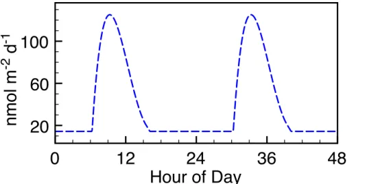
In the PHOTO simulation, the prescribed flux of I₂ was retained for the nighttime, and an additional I2flux was included in the daytime. This was intended to simulate a

light-dependent I2source, which could be due to photochemical reactions in aerosols

20

or at the sea surface, or due to daytime biological production in the sea surface. The daytime source was tuned to achieve average observed daytime IO levels. The total prescribed I2 flux reached a maximum of 125 nmol m

2

d−1, almost a tenfold increase compared to the nighttime flux necessary to reproduce the observed I₂. This maximum flux was reached at about 09:20 h and was set back to the constant (nighttime) flux 25

by shortly after 16:00 (Fig. 7). This simulation matches the daytime IO and nighttime I2

observations reasonably well and predicts a midmorning I₂peak (Fig. 6). The model still does not reproduce daytime I2levels as high as observed, particularly in the afternoon.

(14)

ACPD

13, 25911–25937, 2013

Title Page

Tables Figures

◭ ◮

Back Close

Full Screen / Esc

Discussion

P

a

per

|

D

iscussion

P

a

per

|

Discussion

P

a

per

|

Discuss

ion

P

a

per

of the observed afternoon I₂levels using an extra source of I₂from the surface would result in a late evening peak in IO. Such a peak was not observed. To summarize, the daytime IO and nighttime I2may be explained by the addition of a time-varying surface

I₂ source, but the observed daytime IO and I₂ cannot simultaneously be explained simply by an additional source. We think this lack of agreement is most likely explained 5

by the positive measurement artifact in the daytime I2.

In the HOI simulation, sea-air fluxes of both HOI and I₂ were prescribed without modifcation or optimization after Carpenter et al. (2013). Their sea-air fluxes of HOI are highest at night and the I2 fluxes are highest during the day due to the different

air-sea gradients of the two species between night and day. In the daytime, I₂ levels 10

are extremely low due to rapid photolysis and no known gas phase source. HOI, on the other hand, photolyzes more slowly and can be formed in the gas phase. HOI is also thought to have a significant aerosol sink during the nighttime, as opposed to I2. This

simulation also does a good job representing both the daytime IO and the nighttime I2 mixing ratios, but yielding slightly higher daytime IO and slightly lower nighttime I2

15

than the PHOTO simulation. This simulation does not predict a morning I2 increase.

The HOI case predicts the highest levels of ICl of all the runs, up to 6 pmol mol−1_.

6 Discussion: Ix sources and halogen cycling

The modeling scenarios which best represent the observed inorganic iodine at CVAO are the PHOTO and HOI cases. The laboratory observations of HOI production from 20

seawater ozonolysis provide a strong case that this process should be considered in MBL halogen chemistry. The good agreement between the lab-estimated fluxes and the observational data supports the idea that sea surface-derived HOI is the major source of gas phase inorganic iodine at CVAO. This is therefore also likely the case for all ocean regions not impacted by unusually strong localized emissions (such as 25

(15)

ACPD

13, 25911–25937, 2013

Title Page

Tables Figures

◭ ◮

Back Close

Full Screen / Esc

Discussion

P

a

per

|

D

iscussion

P

a

per

|

Discussion

P

a

per

|

Discuss

ion

P

a

per

|

diurnal cycle required (Fig. 7). While this remains a possibility, the HOI flux is clearly a more straightforward explanation.

Both the PHOTO and HOI cases generate at least 3 pmol mol−1of ICl at night. This is a consequence of HOI uptake in particles followed by reaction with Cl−. ICl was not detected either in 2007 or in 2009, despite monitoring the relevant mass transitions for 5

several days in each case. There is no reason to suspect that the instrument was not similarly sensitive to ICl as to I₂, despite the lack of a specific calibration standard for ICl. Similarly, BrCl has not been observed at CVAO despite evidence for active bromine cycling (Lawler et al., 2009; Read et al., 2008). These observations strongly suggest that current models overpredict the conversion of HOBr and HOI to the interhalogens 10

BrCl and ICl in aerosols. It remains unclear whether all hypohalous acids (including HOCl) undergo significant losses to organic species in particles, or whether the equi-librium reactions among the various dissolved halogen species need to be reexamined.

7 Conclusions

We report the first MBL I2 observations in marine air that is not impacted by coastal

15

macroalgal emissions or sea ice chemistry. The data clearly demonstrate that the very high I2 levels previously reported for coastal air are not representative of open ocean

conditions. The very low observed nighttime levels provide an upper bound for I2

pro-duction by reaction of O₃ on the surface ocean in this region. The “dark” processes producing I2 at night are too slow to explain the levels of IO observed in the

day-20

time, given known iodine recycling mechanisms. The sea-air flux of HOI generated by ozonolysis of seawater and recently proposed by Carpenter et al. (2013) could explain the observations. If this is the case, then IO levels similar to those at CVAO should occur over most of the world oceans. O3-stimulated release of iodine from the sea

sur-face induces catalytic ozone destruction, limiting the lifetime of O3over the oceans. The

25

(16)

ACPD

13, 25911–25937, 2013

Title Page

Tables Figures

◭ ◮

Back Close

Full Screen / Esc

Discussion

P

a

per

|

D

iscussion

P

a

per

|

Discussion

P

a

per

|

Discuss

ion

P

a

per

at CVAO is a challenge to our understanding of aerosol halogen recycling. This dis-crepancy should be addressed with laboratory studies of synthetic and natural halide solutions and with well-calibrated field observations.

Acknowledgements. We thank Cyril McCormick and Luis Mendes Neves for logistical support. This research was funded by the NSF Atmospheric Chemistry program.

5

References

Allen, T. and Keefer, R.: The formation of hypoiodous acid and hydrated iodine cation by the hydrolysis of iodine, J. Am. Chem. Soc., 77, 2957–2960, 1955. 25921

Amachi, S., Muramatsu, Y., and Kamagata, Y.: Radioanalytical determination of biogenic volatile iodine emitted from aqueous environmental samples, J. Radioanal. Nucl. Chem.,

10

246, 337–341, 2000. 25913

Atkinson, H. M., Huang, R.-J., Chance, R., Roscoe, H. K., Hughes, C., Davison, B., Schönhardt, A., Mahajan, A. S., Saiz-Lopez, A., Hoffmann, T., and Liss, P. S.: Iodine emissions from the sea ice of the Weddell Sea, Atmos. Chem. Phys., 12, 11229–11244, doi:10.5194/acp-12-11229-2012, 2012. 25915

15

Carpenter, L. J., Fleming, Z. L., Read, K. A., Lee, J. D., Moller, S. J., Hopkins, J. R., Purvis, R. M., Lewis, A. C., Müller, K., Heinold, B., Herrmann, H., Fomba, K. W., Pinxteren, D., Müller, C., Tegen, I., Wiedensohler, A., Müller, T., Niedermeier, N., Achterberg, E. P., Patey, M. D., Kozlova, E. A., Heimann, M., Heard, D. E., Plane, J. M. C., Mahajan, A., Oetjen, H., Ingham, T., Stone, D., Whalley, L. K., Evans, M. J., Pilling, M. J., Leigh, R. J., Monks, P. S.,

Karuna-20

haran, A., Vaughan, S., Arnold, S. R., Tschritter, J., Pöhler, D., Frieß, U., Holla, R., Mendes, L. M., Lopez, H., Faria, B., Manning, A. J., and Wallace, D. W. R.: Seasonal characteristics of tropical marine boundary layer air measured at the Cape Verde Atmospheric Observa-tory, Journal of Atmospheric Chemistry, 67, 87–140, doi:10.1007/s10874-011-9206-1, 2011. 25916, 25922

25

(17)

ACPD

13, 25911–25937, 2013

Title Page

Tables Figures

◭ ◮

Back Close

Full Screen / Esc

Discussion

P

a

per

|

D

iscussion

P

a

per

|

Discussion

P

a

per

|

Discuss

ion

P

a

per

|

Dixneuf, S., Ruth, A. A., Vaughan, S., Varma, R. M., and Orphal, J.: The time dependence of molecular iodine emission from Laminaria digitata, Atmos. Chem. Phys., 9, 823–829, doi:10.5194/acp-9-823-2009, 2009. 25913

Finley, B. and Saltzman, E.: Observations of Cl₂, Br₂, and I₂in coastal marine air, J. Geophys. Res., 113, D21301, doi:10.1029/2008JD010269, 2008. 25916

5

Gallagher, M., King, D., and Whung, P.: Performance of the HPLC/fluorescence SO₂detector during the GASIE instrument intercomparison experiment, J. Geophys. Res., 102, 16247– 16254, 1997. 25917

Garland, J. and Curtis, H.: Emission of iodine from the sea surface in the presence of ozone, J. Geophys. Res., 86, 3183–3186, 1981. 25913

10

Johnson, C. C.: The geochemistry of iodine and its application to environmental strategies for reducing the risks from iodine deficiency disorders, British Geological Survey Commissioned Report, CR/03/057N, 54 pp., 2003. 25913

Jones, C. E., Hornsby, K. E., Sommariva, R., Dunk, R. M., von Glasow, R., McFiggans, G., and Carpenter, L. J.: Quantifying the contribution of marine organic gases to atmospheric iodine,

15

Geophys. Res. Lett., 37, L18804, doi:10.1029/2010GL043990, 2010. 25913, 25915, 25920, 25923

Lawler, M. J., Finley, B. D., Keene, W. C., Pszenny, a. a. P., Read, K. a., von Glasow, R., and Saltzman, E. S.: Pollution enhanced reactive chlorine chemistry in the eastern tropical Atlantic boundary layer, Geophys. Res. Lett., 36, 1–5, doi:10.1029/2008GL036666, 2009.

20

25916, 25917, 25925

Lawler, M. J., Sander, R., Carpenter, L. J., Lee, J. D., von Glasow, R., Sommariva, R., and Saltzman, E. S.: HOCl and Cl₂ observations in marine air, Atmos. Chem. Phys., 11, 7617– 7628, doi:10.5194/acp-11-7617-2011, 2011. 25921

Lee, J. D., Moller, S. J., Read, K. A., Lewis, A. C., Mendes, L., and Carpenter, L. J.: Year-round

25

measurements of nitrogen oxides and ozone in the tropical North Atlantic marine boundary layer, J. Geophys. Res., 114, 1–14, doi:10.1029/2009JD011878, 2009. 25922

Lee, J. D., McFiggans, G., Allan, J. D., Baker, A. R., Ball, S. M., Benton, A. K., Carpen-ter, L. J., Commane, R., Finley, B. D., Evans, M., Fuentes, E., Furneaux, K., Goddard, A., Good, N., Hamilton, J. F., Heard, D. E., Herrmann, H., Hollingsworth, A., Hopkins, J. R.,

30

(18)

ACPD

13, 25911–25937, 2013

Title Page

Tables Figures

◭ ◮

Back Close

Full Screen / Esc

Discussion

P

a

per

|

D

iscussion

P

a

per

|

Discussion

P

a

per

|

Discuss

ion

P

a

per

K. A., Saiz-Lopez, A., Saltzman, E. S., Sander, R., von Glasow, R., Whalley, L., Wieden-sohler, A., and Young, D.: Reactive halogens in the marine boundary layer (RHaMBLe): The tropical North Atlantic experiments, Atmospheric Chemistry and Physics, 1031–1055, https://uhra.herts.ac.uk/dspace/handle/2299/7734, 2010. 25916, 25922

Mahajan, A. S., Plane, J. M. C., Oetjen, H., Mendes, L., Saunders, R. W., Saiz-Lopez, A., Jones,

5

C. E., Carpenter, L. J., and McFiggans, G. B.: Measurement and modelling of tropospheric reactive halogen species over the tropical Atlantic Ocean, Atmos. Chem. Phys., 10, 4611– 4624, doi:10.5194/acp-10-4611-2010, 2010. 25914, 25915, 25920, 25922

Mahajan, A. S., Whalley, L. K., Kozlova, E., Oetjen, H., Mendez, L., Furneaux, K. L., Goddard, A., Heard, D. E., Plane, J. M. C., and Saiz-Lopez, A.: DOAS observations of formaldehyde

10

and its impact on the HO_x balance in the tropical Atlantic marine boundary layer, J. Atmos. Chem., 66, 167–178, doi:10.1007/s10874-011-9200-7, 2011. 25922

Mahajan, A. S., Gómez Martín, J. C., Hay, T. D., Royer, S.-J., Yvon-Lewis, S., Liu, Y., Hu, L., Prados-Roman, C., Ordóñez, C., Plane, J. M. C., and Saiz-Lopez, A.: Latitudinal distribution of reactive iodine in the Eastern Pacific and its link to open ocean sources, Atmos. Chem.

15

Phys., 12, 11609–11617, doi:10.5194/acp-12-11609-2012, 2012. 25915

McFiggans, G., Coe, H., Burgess, R., Allan, J., Cubison, M., Rami Alfarra, M., Saunders, R., Saiz-Lopez, A., Plane, J. M. C., Wevill, D., Carpenter, L., Rickard, A. R., and Monks, P. S.: Di-rect evidence for coastal iodine particles from Laminaria macroalgae – linkage to emissions of molecular iodine, Atmos. Chem. Phys. Discuss., 4, 939–967,

doi:10.5194/acpd-4-939-20

2004, 2004. 25913, 25914

Neuman, J. A., Nowak, J. B., Huey, L. G., Burkholder, J. B., Dibb, J. E., Holloway, J. S., Liao, J., Peischl, J., Roberts, J. M., Ryerson, T. B., Scheuer, E., Stark, H., Stickel, R. E., Tanner, D. J., and Weinheimer, A.: Bromine measurements in ozone depleted air over the Arctic Ocean, Atmos. Chem. Phys., 10, 6503–6514, doi:10.5194/acp-10-6503-2010, 2010. 25921

25

Palmer, C. J., Anders, T. L., Carpenter, L. J., Küpper, F. C., and McFiggans, G. B.: Iodine and Halocarbon Response of Laminaria digitata to Oxidative Stress and Links to Atmospheric New Particle Production, Environ. Chem., 2, 282, doi:10.1071/EN05078, 2005. 25913 Raofie, F., Snider, G., and Ariya, P. A.: Reaction of gaseous mercury with molecular iodine,

atomic iodine, and iodine oxide radicals Kinetics, product studies, and atmospheric

implica-30

tions, Canadian Journal of Chemistry, 820, 811–820, doi:10.1139/V08-088, 2008. 25913 Read, K. a., Mahajan, A. S., Carpenter, L. J., Evans, M. J., Faria, B. V. E., Heard, D. E.,

(19)

ACPD

13, 25911–25937, 2013

Title Page

Tables Figures

◭ ◮

Back Close

Full Screen / Esc

Discussion

P

a

per

|

D

iscussion

P

a

per

|

Discussion

P

a

per

|

Discuss

ion

P

a

per

|

Saiz-Lopez, A., Pilling, M. J., and Plane, J. M. C.: Extensive halogen-mediated ozone de-struction over the tropical Atlantic Ocean., Nature, 453, 1232–5, doi:10.1038/nature07035, 2008. 25915, 25920, 25925

Read, K. A., Lee, J. D., Lewis, A. C., Moller, S. J., Mendes, L., and Carpenter, L. J.: Intra-annual cycles of NMVOC in the tropical marine boundary layer and their use for interpreting

5

seasonal variability in CO, J. Geophys. Res., 114, 1–14, doi:10.1029/2009JD011879, 2009. 25922

Saiz-Lopez, A. and Plane, J. M.: Novel iodine chemistry in the marine boundary layer, Geophys. Res. Lett., 31, L04112, doi:10.1029/2003GL019215, 2004. 25913

Saiz-Lopez, A., Plane, J. M. C., McFiggans, G., Williams, P. I., Ball, S. M., Bitter, M., Jones,

10

R. L., Hongwei, C., and Hoffmann, T.: Modelling molecular iodine emissions in a coastal marine environment: the link to new particle formation, Atmos. Chem. Phys., 6, 883–895, doi:10.5194/acp-6-883-2006, 2006. 25914

Saiz-Lopez, A., Plane, J. M. C., Mahajan, A. S., Anderson, P. S., Bauguitte, S. J.-B., Jones, A. E., Roscoe, H. K., Salmon, R. A., Bloss, W. J., Lee, J. D., and Heard, D. E.: On the vertical

15

distribution of boundary layer halogens over coastal Antarctica: implications for O₃, HO_x, NO_x and the Hg lifetime, Atmos. Chem. Phys., 8, 887–900, doi:10.5194/acp-8-887-2008, 2008. 25912, 25913, 25922

Saiz-Lopez, A., Plane, J., Baker, A., Carpenter, L., von Glasow, R., Gómez Martín, J., McFig-gans, G., and Saunders, R.: Atmospheric chemistry of iodine, Chem. Rev., 112, 1773–1804,

20

doi:10.1021/cr200029u, 2012. 25915

Saunders, R. W., Kumar, R., Gómez Martín, J. C., Mahajan, a. S., Murray, B. J., and Plane, J. M. C.: Studies of the Formation and Growth of Aerosol from Molecular Iodine Precursor, Zeitschrift für Physikalische Chemie, 224, 1095–1117, doi:10.1524/zpch.2010.6143„ 2010. 25914

25

Vogt, R., Sander, R., Glasow, R. V. O. N., and Crutzen, P. J.: Iodine Chemistry and its Role in Halogen Activation and Ozone Loss in the Marine Boundary Layer: A Model Study, J. Atmos. Chem., 32, 375–395, 1999. 25912, 25921

von Glasow, R.: Tropospheric Halogen Chemistry, in: Treatise on Geochemistry, Volume 4, edited by: Keeling, R. F., 21–64, Elsevier, 2003. 25912

30

(20)

ACPD

13, 25911–25937, 2013

Title Page

Tables Figures

◭ ◮

Back Close

Full Screen / Esc

Discussion

P

a

per

|

D

iscussion

P

a

per

|

Discussion

P

a

per

|

Discuss

ion

P

a

per

(21)

ACPD

13, 25911–25937, 2013

Title Page

Tables Figures

◭ ◮

Back Close

Full Screen / Esc

Discussion

P

a

per

|

D

iscussion

P

a

per

|

Discussion

P

a

per

|

Discuss

ion

P

a

per

|

air gate valves

scrubber

ground 2.9 m

standard addition

2 in ABS pipe

air

2.5 m

to CIMS (63 SLPM) to CIMS (63 SLPM)

overﬂow

air air

gate valves

scrubber

ground 8.2 m

5.7 m

1.6 m 6 in ABS

pipe

2 in ABS pipe

air

a. b.

sample ﬂow (130 SLPM)

(22)

ACPD

13, 25911–25937, 2013

Title Page

Tables Figures

◭ ◮

Back Close

Full Screen / Esc

Discussion

P

a

per

|

D

iscussion

P

a

per

|

Discussion

P

a

per

|

Discuss

ion

P

a

per

140 142 144 146 148

Day of Year (140 = May 20, 2007) 0

0.2 0.4 0.6

I2

(pmol mol

-1) 5 7 9

Windspeed (m s

-1)

25 35 45

O3

(nmol mol

-1) 35 45 55

Wind Origin (

˚

)

Fig. 2.Wind speed, wind direction, O₃mixing ratios, and I₂mixing ratios at CVAO during May

(23)

ACPD

13, 25911–25937, 2013

Title Page

Tables Figures

◭ ◮

Back Close

Full Screen / Esc

Discussion

P

a

per

|

D

iscussion

P

a

per

|

Discussion

P

a

per

|

Discuss

ion

P

a

per

|

140 141 142 143 144 145 146

Day of Year (140 = May 20, 2009) 0

0.4 0.8 1.2 1.6

I2

(pmol mol

-1) 4 6 8 10

Windspeed (m s

-1)

30 40 50

O3

(nmol mol

-1)

0˚

20 40 60

Wind Origin (

˚

)

Fig. 3.Wind speed, wind direction, O₃ mixing ratios, and I₂ mixing ratios at CVAO during one

(24)

ACPD

13, 25911–25937, 2013

Title Page

Tables Figures

◭ ◮

Back Close

Full Screen / Esc

Discussion

P

a

per

|

D

iscussion

P

a

per

|

Discussion

P

a

per

|

Discuss

ion

P

a

per

148 149 150 151 152 153 154

Day of Year (148 = May 28, 2007) 0

400 800 1200 1600

Raw I

2

signal (arbitrary units)

(25)

ACPD

13, 25911–25937, 2013

Title Page

Tables Figures

◭ ◮

Back Close

Full Screen / Esc

Discussion

P

a

per

|

D

iscussion

P

a

per

|

Discussion

P

a

per

|

Discuss

ion

P

a

per

|

12:00 18:00 00:00 06:00

Time of day 0.05

0.1 0.15 0.2 0.25 0.3

I2

mixing ratio (pmol mol

-1)

Fig. 5.Mean hourly binned I₂mixing ratios measured over three weeks at CVAO in 2007. Error

(26)

ACPD

13, 25911–25937, 2013

Title Page

Tables Figures

◭ ◮

Back Close

Full Screen / Esc

Discussion

P

a

per

|

D

iscussion

P

a

per

|

Discussion

P

a

per

|

Discuss

ion

P

a

per

0 12 24 36 48

Time (Hours) 0

0.02 0.04 0.06 0.08 0.1

IBr (pmol mol

-1 )

0 12 24 36 48

Time (Hours) 0

2 4 6

ICl (pmol mol

-1 )

0 12 24 36 48

Time (Hours) 0

1 2

IO (pmol mol

-1 )

0 12 24 36 48

Time (Hours) 0

0.1 0.2 0.3

I2

(pmol mol

-1 )

Fig. 6.THAMO box model results for four simulations. BASE (halocarbons only): black solid

(27)

ACPD

13, 25911–25937, 2013

Title Page

Tables Figures

◭ ◮

Back Close

Full Screen / Esc

Discussion

P

a

per

|

D

iscussion

P

a

per

|

Discussion

P

a

per

|

Discuss

ion

P

a

per

|

Observations of I<sub>2</sub> at a remote marine site

ACPD

Observations of I

2

at a remote marine site

ACPD

mag-ACPD

ACPD

ACPD

ACPD

ACPD

ACPD

ACPD

ACPD

ACPD

ACPD

ACPD

ACPD

ACPD

ACPD

ACPD

ACPD

ACPD

ACPD

ACPD

ACPD

ACPD

ACPD

ACPD

ACPD

ACPD

0

12

24

36

48

Hour of Day

20

60

100

nmol m

-2

d

-1

₂