A New Approach to the Data Aggregation in Wireless
Sensor Networks
Chamran Asgari
Department of Computer Engineering, Islamic Azad University, Arak Branch, Arak, Iran
Javad Akbari Torkestani
Young Researchers Club, Arak Branch, Islamic Azad University, Arak, Iran
Abstract
S
everal algorithms have been developed for problems of data aggregation in wireless sensor networks, all of which tried to increase networks lifetime. In this paper, we deal with this problem using a more efficient method, and offer a heuristic algorithm based on distributed learning automata to solve data aggregation problems within stochastic graphs. Given that data aggregating through creating backbones and making connected dominating sets (CDS) in networks lowers the ratio of responding hosts to the hosts existing in virtual backbones, we employed this idea to our algorithm, trying to increase networks lifetime considering such parameters as sensors lifetime, remaining and consumption energies in order to have an almost optimal data aggregation within networks. Finally, we assess our algorithm for make CDS lifetime given increased transmission range and increased sensors number.Keywords: Wireless sensor network, Data aggregation, Connected Dominating Set, Backbone formation, distributed learning automata.
1. Introduction
Wireless sensor networks consist of a large number of inexpensive sensor nodes distributed in environment uniformly, having limited energy, therefore, in the most cases, nodes communicate with central node via their neighbors [1]. On the other hand, an optimal route must be selected because there are different routes to central node from any other nodes. On the other hand, frequent use of one route results in reduction of energy of sensors located on that route and, ultimately, in sensors destruction. For solving this problem, we can consider a wireless sensor network as a graph in the nodes (hosts) which are the sensors and edges show the links between sensors. If a backbone can be created in this graph the constituent nodes that are able to communicate with all graph nodes or, in other words, to cover them, it is not necessary to use all graph nodes to aggregate the data and it suffices only to carry out data aggregation on backbone nodes, then, to send the result in the form of a single packet to central node. The set of nodes
constituting backbone are referred to Connected Dominating Set (CDS) and each node of this set is called dominator. Creating CDS to aggregate data is a promising approach for reducing routing overhead since messages are transmitted only within virtual backbone by means of CDS and, also, data aggregating through lowers the ratio of responding hosts to the hosts existing in virtual backbones [2-5]. By offering an intellectual algorithm, we tried to increase networks lifetime considering such parameters as sensors lifetime, remaining and consumed energies of sensors, in order to have an almost optimal data aggregation within networks. Our algorithm operates as follows: initially, wireless sensor network is modeled as a unit disk graph G= (V, E) in the nodes that represent hosts and edges show the links among hosts [6, 7]; then, an intellectual algorithm based on distributed learning automata is implemented on the model to aggregate data. For this algorithm, each host is equipped with a learning automaton. Sink node is considered as the first dominator here. Next, learning automata selects next action randomly from its variable action set with respect to action probability vector and this process continues until finally entire network is covered, with set of selected dominators constituting the backbone. After that, message "data aggregation" is sent to dominators from sink node inside backbone. Dominators will send the message to their parents immediately after receiving it. Each parent must wait until it receives data from all its children, then, aggregates all data received from its children and sends it to its own parent until aggregates data is sent to sink node in the form of a single packet.
Once every iteration of the process has finished, action probability vectors are updated for any learning automata. Eventually, with iteration of process, learning automata converges to public policy of optimal data aggregation for network graph. Given that lifetime of created CDS is of special importance, the algorithm will pursue the aim of choosing a CDS with the longest lifetime from made CDSs.
be presented. In the Section 4, the proposed DLA-based backbone formation algorithm for finding a CDS with longest lifetime is presented. The experiment results are demonstrated in the section 5 and finally are in the section 6, the conclusion and future work is highlighted.
2. Related work
Many routing algorithms have been provided for the sensor networks. For some of these algorithms, each node may has more than one route to sink node that one of them is selected on the basis of a series of criteria, among the level of energy consumption along the route can be a proper criterion. Energy saving can be taken into account in two ways: (1) energy consumption is calculated for any separate routes, then, the route with minimal energy consumption is chosen [8]; and (2) data aggregation is based on provided learning automata, which prevents extra packets from being sent in networks by identifying sensors generating identical data and by activating sensor nodes periodically, and saves a large amount of energy while increasing network lifetime [9]. A solution has been provided in [10] for data aggregating and routing with intra network aggregations in wireless sensor networks in order to maximize network lifetime by using intra network processing techniques and data aggregation. The relationship between the security and data aggregation process within wireless sensor networks has been investigated in [11].
In [12], network is first clustered in order to aggregate data, then, head- clusters aggregate data from each cluster separately. A network organized into clusters with the same sizes results in unequal load distribution among head- cluster nodes. But [12] provides a model in which clusters are of different sizes, resulting in more uniform energy distribution among head-cluster nodes and with increasing in network lifetime. In [13] has offered data aggregation in wireless sensor networks by using ant colony algorithm that states the problem of creating data aggregation tree in wireless sensor networks for a group of source nodes to send sensed data to the single sink node. Ant colony system represents a natural method of heuristic search to determining data aggregation. Each ant discovers all possible routes to sink node and data aggregation tree is created by using accumulated pheromone. In [14] provides two different tree structures LPT and E-Span to facilitate aggregation of data in wireless sensor networks. In LPT, nodes having more remaining energy are chosen as aggregation parents. The tree is restructured when one node has no long function or when a broken link is identified. E-Span is an aware energy–spanning tree algorithm in which source node with maximal remaining energy is selected as root. Other source nodes select their corresponding parents from their neighbors on the basis of such information as
remaining energy and distance to root. In [15] an efficient energy–spanning tree is used to aggregate data in wireless sensor network for making which two parameters are used: energy and distance [15] uses route energy average to balance parameters energy an distance while previously provided algorithms have selected only one of these parameters as the main one and gave sound priority to the other. In [16] unlike common data aggregation methods, ESPDA avoids transmitting redundant data to head–clusters from sensor nodes in order to remove redundancy for improving application of efficient energy and bandwidth in sensor nodes . In [17] presents a scheme of efficient and highly accurate energy to aggregate data securely. The main idea of this is to aggregate data carefully without disclosing or reading secret information of sensors and posing considerable overhead in energy–limited sensors.
In [18] aggregation of data in wireless sensor networks is raised to balance latency and communication cost. In [19] spanning tree- based algorithms are provided to create high convergence between data aggregation and efficient energy and low latency in wireless sensor networks. Initially [19] provides two algorithms for making DAC tree. The first algorithm is the kind of minimum spanning tree, and the second of individual source shortest path spanning tree. Both of them are used as combined (COM) algorithm stimulator generally based on MST and SPT.
3. Preliminaries
Before presenting the algorithm, it is necessary to offer some primary definitions and concepts as follows.
3.1 Connected dominating set
Dominating set S of graph G = (V, E) is a host subset so that each host exists in set S or is adjacent to a host from S. In dominating set S, each host is referred to as dominator host, otherwise, as dominate host. A minimum dominating set is one with minimum cardinality. A connected dominating set S from graph G is one connected to each other. A minimum connected dominating set is a CDS with minimum cardinality.
3.2 Calculating sensors and CDS lifetimes
Let be the number of sensors: be initial energy of sensors; , be the number of bits being routed from sensor to sensor ; , be the number of bits being routed from sensor to base station; , be sensor communication cost of transmitting one bit to sensor ; and , be sensor communication cost for receiving one bit from sensor j [22]. In data aggregation process, each sensor receives data from one or more sensors, but sends data only to one sensor. Total sensor consumed energy amount for transmitting one event is calculated as follows:
, , , ,
And sensor remaining energy amount is calculated as follows:
And are current and previous remaining energies, respectively.
Also, sensor lifetime is calculated as follows:
⁄
The average of CDS lifetime is calculated as follows:
⁄
Where equal to CDS lifetime average and equal to Total lifetime of sensors constituting CDS which is calculated as follows:
In (4) and (5) equations is the number of sensors exist in CDS.
3.3 Learning automata
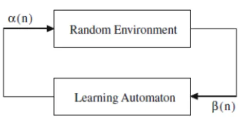
A learning automata (LA) [23-25] is an abstract model capable of doing finite actions. Each selected action is evaluated by a probable environment, the result that is delivered to automata in the form of a positive or negative signal. Learning automata use this response to select their next action. Ultimate goal is for automatas to select the best of their actions. The best action is one maximizing the likelihood of receiving rewards from environment.
The Probable environment can be expressed
mathematically by triple , , where
, , … , is the set of environment inputs and , , … , is each action's being penalized. Fig. 1 shows the relationship between learning automate and environment.
Fig. 1 the relationship between learning automata and environment
Given the values of , three different models are defined for probable environments. Whenever is a two-members set of [0, 1], the environment is of type , that is, values of and is selected as environment outputs. In this case, means "being penalized" and means "being rewarded".
If is a value bounded to [0, 1], the model is of type ; and if is a stochastic variable within [0, 1], the environment is of type S. represents the probability that action receives an undesirable response from environment. The values of do not change in static environments with changing the time in non- static ones [26].
Learning automatas are divided into two groups: (a) those with fixed structured, and (b) those with variable structured. In this paper, we make use of the variable structured. For learning Automatas with fixed structures, probabilities of automata actions are fixed while, for learning automatas with variable structures, they are updated with each turn of iteration. Learning automatas with variable structures can be denoted by
triple , , , where , , … , is an
automata's actions set; , , … , is its inputs; , , … , is probability vector of each automata's action; and
, , is learning algorithm. Automatas choose their actions randomly on the basis of probability vector and exercise. It is on the environments that they get a response. If the actions selected by Learning automate is action , then, automata updates its action probabilities to Eq. 6 in the case of receiving desirable response from environment while it does this according to Eq. 7 in the case of receiving undesirable one.
,
,
Where is the number of automata's actions and is penalty parameter. There following algorithms can be available on the basis of different values considered for parameters and of learning:
2) If the value of is many times smaller than that of , resulting learning method is called liner reward epsilon scheme _ .
3) If , algorithm is called linear reward inaction _
3.3.1 Distributed learning automata (DLA)
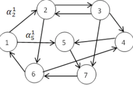
A distributed learning of automata (DLA) [27, 28] is a network of LAs cooperating to solve a particular problem. Within this network of cooperating automata, only one automata is active at a time. In DLA the number of actions each automata is able to do is equal to the number of automatas connects to that one. When an automata selects an action in the network, other automata connected to it is activated. In other words, Choosing an action by an automata in this networks corresponds to activation of another automata there. The model considered for DLA network is graph each vertex of which is an automata, as shown in fig. 2 In this graph, presence of edge ( , ) means that choosing the action by activate . The number of actions can select is
denoted as , , … , . within this set,
represents probability related to action . Selecting the action by activates . Shows the number of actions is able to do.
Fig. 2 Network of distributed learning automatas
4. Forming virtual backbone based on distributed learning automata
Suppose that wireless sensor network includes a group of wireless hosts having transmission range and linking, directly or indirectly, to each other. Here, suppose that topological graph corresponds with unit graph where host corresponds with vertex . Any two hosts connected to each other are said to be neighbors having mutual communication. Therefore, it is assumed that network graph is a undirected graph. Each host has a unique argument and is required to know its neighbors. In this section, an algorithm based on distributed learning automata is provided for data aggregating in wireless sensor networks, focusing on finding an almost optimal solution for problem of data aggregation in network graph. In this approach, each host (e.g. ) is equipped with learning automata (e.g. ). A network of
learning of automata is denoted by binary , where , , … , indicates set of learning automatas corresponding to set of vertexes (hosts) and
, , … , represents action set. And also,
, , … , represents an action set which can be run by learning automata . Here, we use learning automata with variable actions the number of which depends on the number of adjacent vertexes (neighbors) of respective learning automata.
4.1 Action set formation method
In the algorithm provided for forming action set related to learning automata , initially, its host (e.g. ) sends a message locally to its neighbors one step apart locally. Hosts located in transmission range from sending host respond to it upon receiving the message and send back their action sets to primary sending host which creates its own action set on the basis of responses received from neighbors. Therefore, each host the message of which was responded adds action to action set of learning automata . In fact, when sends a message to which sends back its response to , the learning automata corresponding to adds action (selection of vertex j ( )) to action set of its own corresponding automata (namely, ). Selection of action corresponding to as dominator is performed by learning automata . So the size of each learning automata action set depends on the order of respective host, assuming that hosts have been distributed in network uniformly. A problem with above defined action set , in which the number of actions is fixed and does not change with time , may result in frequent selection of a host, with virtual backbone including redundant loops and dominators . Therefore, fixed action sets decrease convergence speed of algorithm and enlargethe size of virtual backbone. To overcome these shortcomings, we suggest learning automata with variable actions and present following rules for pruning action set of learning automata.
Rule1. To avoid choosing the same dominators (by different hosts), each activated learning automaton is allowed to prune its action-set by disabling the actions corresponding to the dominator hosts selected earlier. This rule increases the convergence speed, and consequently, decreases the running time of the proposed algorithm.
Rule2. To avoid the loops and the redundant
dominator hosts by no more (dominate) hosts can be spanned; the proposed algorithm prunes the action-set as follows.
all have been spanned (or added to the dominate set) before (see Fig. 4a–f), if any. This rule reduces the dominator set (backbone) size, decreases the running time and improves the convergence rate of algorithm.
4.2 Algorithm description
As mentioned above, we consider our network as a unit disk graph that is, sending radiuses of all graph nodes are equal. Also, we assume the nodes are distributed in network graph randomly. Each of sensor nodes possesses some amount of energy being approximately the same for all nodes at first. Over time, the level of nodes energy changes. In this network, sensor nodes have some information about themselves and their neighboring nodes, including their energy level at a given time, which is updated periodically. As stated earlier, nodes participating in CDS are referred to as dominators and the rest are dominates. We create CDS in accordance with energy levels of network nodes. In fact, we use nodes with higher levels of energy to create CDS. Our aim is actually to make created route more permanent. In other words, we want to increase created CDS lifetime. Each node of network is equipped with learning automata; therefore, we have a network of learning automata each of which has a selected action set. The numbers of each automaton's operations are equal with the number of nodes neighboring the node corresponding to targeted automata that can select only one action from its action set at a moment over time. Given the decrease in nodes energies, we calculate their energy periodically. The amount of energy consumed for sending or receiving a message differs. The amount of energy usually consumed to send a message is much more than that consumed to
receive it. These nodes not located on the route of made CDS go into idle (or sleep) state in which their consumption energy is near zero, thus, energy consumption is associated with nodes located on the route of made CDS. A CDS is made any time the algorithm is iterated. Initially, we define an energy threshold for nodes existing in network, which is the least amount of energy needed by each network node which is for network permanence.
The level of energy of each of nodes located on made CDS route should not be less than this amount of energy defined as threshold level. If so, learning automata of nodes located on the route are penalized, if not, are rewarded. So that the probability of selecting these nodes to make future CDS routes increases. The process of CDS–making continues until made CDS converges toward an optimal response. The pseudo code of algorithm is presented below (Fig. 3). Here, m and k represent the number of nodes constituting CDS and the number of steps of making CDS, respectively.
Is dynamic threshold at kth step; is calculated with Eq. 8. CDS is the selected connected dominating set; W is the weight of made CDS and calculated with Eq. 9 ; VA is the vertex corresponding to learning automata A ; NVA represents neighbors adjacent to vertex (V); and is the number of CDSs made until step .
Algorithm for forming a CDS with maximum of lifetime 1: Input: Graph , , , P ,Iteration_max 2: Output: Optimal nearest Data aggregation 3: Assumptions
4: let CDS denotes the selected connected dominated set 5: Begin algorithm
6: , 7: Repeat
8: , _ , _ , _
9: the automaton corresponding to sink node is selected , denoted as A and activated ,
10: _ _ , _ _ ,
,
11: Repeat
12: If _ && Then
13: Path induced by active automata is traced back for finding an automata with available actions 14: the found learning automata is denoted as A
15: End If
16: Each automata prunes its action set 17: automaton A chosen one of its actions
18: _ _ , _ , _ ,
, ,
19: automaton A is active 20: set A to A
22: , 23: Data aggregation
24: compute the average weight of CDS and denote it 25: Then
26: Reward the selected actions of the activated automata along the CDS 27: Else
28: Penalize selected actions of the activated automata along the CDS 29: End If
30: /
31:
32: Enable all the disabled actions
33: until _
34:End Algorithm
Fig. 3 The pseudo code of proposed algorithm
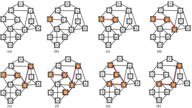
Fig. 4a-e illustrates the steps of making backbone in the first implementation of the algorithm. In fig. 4b, node is considered as sink node and the first dominator. In this case, nodes , , are added to dominate set. In fig. 4c, node is selected as next dominator and node 6 is added to dominate set. In fig. 4d, node is selected as next dominator and nodes , , are added to dominate set. In fig. 4e node is selected as next dominator and node is added to dominate set. Up to this step, we have dominator set of
, , , and dominate set of , , , , , , , , , . Entire
network is not still covered because the size of dominate set is smaller than network's; therefore, the algorithm performs backtracking and selects node as next dominator, hence nodes added to dominate set (fig. 4f). Now, we have dominator and dominate sets of , , , , and of , , , , , , , , , , , , and entire network is covered. Fig. 4g and 4h were obtained in the second and third implementation of algorithm, respectively, that node is considered as sink node and the first dominator.
Fig. 4 The step-by-step backbone formation process
5. Simulation results
In this paper, NS2 software was used to simulate wireless sensor network. Simulation was performed in
a square area of with ,
nodes distributed uniformly in the environment. We assumed learning rate is . and initial energy is 500mj
for each node. Also, we assumed each node consumes 6mj and units of energy to send and receive any kinds of packets, respectively. For this simulation, the
threshold of CDS process and max iteration were set at
. and , respectively. In here, for assessing our algorithm (CDS-LT), we compare our algorithm with proposed algorithms in [14] and [19]. In [14] Lee and Wong have proposed two different tree structures LPT and E-Span to facilitate aggregation of data in wireless sensor networks. In LPT, nodes having more remaining energy are chosen as aggregation parents. The tree is restructured when one node has no long function or when a broken link is identified.
high convergence between data aggregation and efficient energy and low latency in wireless sensor networks. Initially [19] provides two algorithms for making DAC tree. One of the algorithms is the kind of individual source shortest path spanning tree. In here, we evaluate our simulation with respect to made CDS lifetime by expanding transmission range and increasing the number of nodes. We assume transmission range changes from . As it is
show in fig. 5, the CDS lifetime decreases when the transmission range increase. And CDS lifetime decreases by increasing the number of nodes. Also with comparing our algorithm (CDS-LT) with proposed algorithms in [14] and [19] will determine how much our method performs well.
Fig. 5 Comparison CDS life time for CDS-LT algorithm
6. Conclusion
This paper is provided on heuristic algorithm based on distributed learning automata to solve problems of data aggregation in stochastic graphs. Given that data aggregating by creating backbones and making CDSs in networks lowers the ratio of responding hosts to the hosts existing in virtual backbones, we used this idea in our algorithm and tried to find CDSs with the
longest lifetime considering such parameters as lifetime, remaining and consumption energies of sensors in order to have an optimal data aggregation. Simulation results showed that lifetime of made CDSs decreased as the number of nodes increased and transmission range expanded. Also, we compared our algorithm with proposed algorithms in [14] and [19], as shown above our algorithm always outperforms the others in terms of the life time.
References
[1] P. Gupta, and P. R. Kumar, "The capacity of wireless networks", IEEE Transaction on Information Theory, Vol. 46, No. 2, 2000, pp. 388–404.
[2] Y. Z. Chen and A. L. Liestman, "Approximating minimum size weakly connected dominating sets for clustering mobile ad hoc networks", in: Proceedings of the Third ACM International Symposium on Mobile Ad Hoc Networking and Computing, 2002, pp. 157–164.
[3] J. Wu, F. Dai, M. Gao and I. Stojmenovic, "On calculating power-aware connected dominating sets for efficient routing in ad hoc wireless networks", Journal of Communications and Networks, Vol. 4,No. 1,2002.
[4] Y. P. Chen, and A. L. Liestman, "Maintaining weakly-connected dominating sets for clustering ad hoc networks, Ad Hoc Networks, Vol. 3, 2005, pp. 629– 642.
[5] B. Han, and W. Jia, "Clustering wireless ad hoc networks with weakly connected dominating set", Journal of Parallel and Distributed Computing,Vol. 67, 2007, pp. 727–737.
[6] B.N. Clark, C.J. Colbourn and D.S. Johnson, "Unit disk graphs", Discrete Mathematics, 86, 1990, pp. 165–177.
[7] M.V. Marathe, H. Breu, H. B. Hunt III, S. S. Ravi and D. J. Rosenkrantz, "Simple heuristics for unit disk graphs", Networks,Vol. 25, 1995, pp. 59–68.
[8] R. Shah, and J. Rabaey, "Energy Aware Routing for Low Energy Ad Hoc Sensor Networks", Communication /Computation Piconodes for Sensor Networks, 2002.
[9] M. Esnaashari and M. R. Meybodi, "Data Aggregation in wireless Sensor Networks using Learning Automata", Wireless Netw,vol.16, 2010,pp. 687-699. [10] A. Karaki, and R. Ui-Mustafa, et al, "Data aggregation
[11] S. ozdemir and Y. Xiao. "Secure data aggregation in Wireless Sensor Networks:A comprehensive overview" computer Networks, 2009, pp. 2022-2037. [12] S. Soro and W. B. Heinzelman, "Prolonging the
Lifetime of Wireless Sensor Networks via Unequal Clustering", IEEE, pp. 2005.
[13] W. H. Liao, Y. Kao,and et al. "Data aggregation in wireless sensor networks using ant colony algorithm." Network and Computer Applications, 2008, 387-401. [14] W. M. Lee and V. W. S. Wong, "E-Span and LPT for
data aggregation in wireless sensor networks", Computer Communications, 2006, pp. 2506-2520. [15] Z. Esjkandari, M. H. Yaghmaee, et al, "Energy
Efficient Spanning Tree for Data Aggregation in wireless sensor networks", IEEE, 2009.
[16] H. Cam, S. Ozdemir, and et al, "Energy-efficient secure Pattern based data aggregation for wireless sensor networks", Computer Communications, 2006, pp. 446-455.
[17] H. Li, K. Lin, and et al, "Energy-efficient and high-accuracy secure data aggregation in wireless sensor networks", Computer Communications, 2010. [18] P. Korteweg, A. Marchetti-Spaccamela, and et al,
"Data aggregation in sensor networks:Balancing communication and delay costs", Theoretical Computer Science, 2009, pp. 1346-1354.
[19] S. Upadhyayula and S. K. S. Gupta, "Spanning tree based algorithms for low latency and energy efficient data aggregation enhanced convergecast(DAC) in wireless sensor networks", Ad Hoc Networksvol. Vol. 5, 2007, pp. 626-648.
[20] K. M. Alzoubi, P. J. Wan and O. Frieder, "Maximal independent set, weakly connected dominating set, and induced spanners for mobile ad hoc networks", International Journal of Foundations of Computer Science, Vol. 14, No. 2, 2003, 287–303.
[21] S. Basagni, M. Mastrogiovanni, C. Petrioli, "A performance comparison of protocols for clustering and backbone formation in large scale adhoc network", in: Proceedings of the First IEEE International Conference on Mobile Ad Hoc and Sensor Systems, 2004, pp. 70–79.
[22] J. C. Dagher, M. W. Marcellin and M. A. Neifeld, "A Theory for Maximizing the Lifetime of Sensor Networks", IEEE Transaction on Communications, Vol. 55, No. 2, 2007.
[23] K. S. Narendra and K. S. Thathachar, "Learning Automata: An Introduction", Prentice-Hall, New York, 1989.
[24] M. A. L. Thathachar and P. S. Sastry, "A hierarchical system of learning automata that can learn the globally optimal path", Information Science, Vol. 42, 1997, pp. 743–766.
[25] M. A. L. Thathachar and B. R. Harita, "Learning automata with changing number of actions", IEEE Transactions on Systems, Man, and Cybernetics SMG, Vol. 17, 1987, pp. 1095–1100.
[26] S. Lakshmivarahan and M. A .L. Thathachar, "Bounds on the convergence probabilities of learning automata", IEEE Transactions on Systems,Man, and Cybernetics SMC, Vol. 6, 1976, pp. 756–763. [27] K. S. Narendra and M. A .L. Thathachar, "On the
behavior of a learning automaton in a changing environment with application to telephone traffic routing", IEEE Transactions on Systems, Man, and Cybernetics SMC, Vol. 10, No. 5, 1980, pp. 262–269.
[28] H. Beigy and M. R. Meybodi, "Utilizing distributed learning automata to solve stochastic shortest path problems", International Journal of Uncertainty, Fuzziness and Knowledge-Based Systems, Vol. 14, 2006, pp. 591–615.
Chamran Asgarireceived the B.S.
and M.S. degrees in Computer
Engineering in and ,
respectively, Arak, Iran. His research interests include data aggregation algorithms in wireless sensor networks, learning systems, parallel algorithms,
virtual Backbone formation and
minimum spanning tree.