ISSN 1549-3636
© 2007 Science Publications
Topology Discovering and Power saving Mechanism for Routing in a
Tree of Ad-hoc Wireless Networks
Arwa Zabian
Department of CIS, Irbid National University, Irbid, Jordan
Abstract: Power management in mobile network is an open challenges where the power level in the network influences the network life time. However, there are a trade off between the power consumption and the connectivity in mobile networks. We present a topology control mechanism and a routing protocol for Ad-Hoc wireless networks that chooses the shortest path given the lower power consumption. The power consumption in forwarding a packet in the proposed topology is depends on only two main factors are the number of hops and the packet size. Our analytical results are confirmed by our simulation results where both has give the same results for power consumption in sending a packet taking in consideration only the power consumed in communication.
Keywords : Power saving, dynamic tree, dynamic routing protocol, topology discovering for mobile networks.
INTRODUCTION
In wireless communications networks, energy consumption is a major performance metric, lower is the energy consumption longer is the network life time. Thus, there are an increasing interest in power saving. Since energy conservation is not an issue of one particular layer of the network protocols stack. Many researches have focused on cross layer design to conserve energy more effectively. One such effort is to employ power control at the MAC layer and to design a power aware routing at the network layer. Power control is a mechanism that varies the transmission power level when sending packets. The primary benefit of power control is to increase channel capacity. The secondary benefit is to conserve energy in a manner to increase the system life time as possible. One possible way to reduce energy consumption is to exchange RTS/CTS packets at maximum power and to send their DATA/ACK packets at minimum power needed for reliable communications. The transmission power determines the range over which the signal can be coherently received, and is therefore crucial in determining the performance of the network ( throughput, delay, and energy consumption).
However, reducing then transmission range increases the number of hops between the source and the destination but reduces the area of transmission and allows more concurrent transmission in the same neighborhood. In addition, reducing the transmission range reduces the energy required to deliver a packet. While, increasing the transmission range increases the number of nodes reachable by only one communication and increases the power consumption. That means,
there is a trade off between energy saving and the network performance. So, The design of the power management framework in wireless ad-hoc network is a challenging research problem, where the energy conservation usually comes at the cost of degraded performance. Any solution must address the following performance goals:
1. minimizing the impact on capacity, throughput, packet and route latency.
2. minimizing the overhead imposed by energy management scheme .
3. maximizing the system life time.
power consumption for all the network. The problem studied in this paper can be considered as an instance of the MECBS problem where we try to adjust the transmission power of each node in a manner to reach a subset of nodes by only one hop, reducing in that the power consumption in the routing of a packet. In addition , we propose a routing protocol that constructs to each node a vector based on the transmission cost on each of its outgoing link. Then the routing of a message is done given the shortest path in term of power consumption. This paper is organized as follow: Section 2, present the Topology Discovering Algorithm (TDA) and its properties. Section 3, contains the power consumption mechanism proposed for the topology determined by TDA. Section 4, present an aware routing protocol. Section 5, present our results. Section 6. give an overview of the previous works in the area studied., Finally conclusions and future works.
Topology discovering Algorithm (TDA)
System Model: The system is composed of a set of mobile nodes organized in clusters. Our system is modeled by a graph G = (V,E), where V is the set of nodes of the network, |V| = n, and E is the set of bidirectional links that satisfy the following condition:
∀ a,b ∈ V, a link a ↔ b ∈E exists, if and only if the
Euclidean distance between a and b is less or equal to the transmission range l: |xa-x b| ≤ l where xa , x b are the location of the nodes a, b respectively.
Assumptions
• We assume that the system is composed of set of
mobile nodes equal in transmission range and power consumption. That means, the power consumed by each node for the packet transmission is the same.
• Each node in the system can be only in two states:
active or down. Active node means, can carry out a communication for itself or for the other nodes. A node is considered down, when its battery is to be exhausting or is in sleep state. In this case, it must inform its neighbors about that and it will be marked as down.
For interference reasons, we propose some constrains on the number of children of each node, by limiting it to be at most 5. This reduces the interferences between them, and keeps a good balance between the network density and the connectivity, and takes in consideration the mobility issues. In addition, for mobility management reason, each node maintains some additional link (at most 3) between siblings (we define
sibling as the children of the same parent or different parents at the same level).
Topology Discovering Algorithm (TDA): In this section, we will present our proposed topology that is constructed by our proposed algorithm Topology Discovering Algorithm (TDA) [24]. In which , given a graph G, TDA constructs a tree leveled by the transmission range. That means, all the children are in the transmission range of the parent node. After constructing the previous tree, a packet sent from a given source to any destination travels at most h hops that is the height of the tree. In that, we reduce the number of exchanged messages for the topology maintenance, and we give an upper bound of the energy consumption for packets transmission.
The algorithm works in phases, and is structured similarly to NDA (Neighbor Discovering Algorithm) 23], proposed for wired networks .TDA runs in two phases: discovering phase and monitoring phase.
In the first phase, the root node discovers its environment and determines the nodes that collaborate with it. And in the second phase each node collects information about its neighbors.
Discovering phase:
1. In this phase, a node S denoted as root starts discovering its neighborhood by broadcasting a hello message and setting a time out t.
2. t is equal to the time needed for a message to travel a distance 2l, plus to it the processing time (the time needed to take a decision to collaborate or not), where l is the maximum distance traveled by the radio signal given the node transmission range (E ≈ r α≈ 1/dα) where 2 ≤α≤4.
3. All the response messages received will be buffered in a list Q based on the arriving time.
4. After the time out is over, S selects the responses numbering the sender nodes from 1 to k, where k is the number of desired children, in the tree and 2
≤ k ≤ 5 . All the nodes with k>5 will be deleted
from Q.
5. If the time out is over and no messages arrived, S waits a time equal to t and restarts the discovering phase, until the construction of its subtree or until receiving a broadcast message from other nodes. 6. If a node A receives a hello message and it wants to
In the discovering phase, S encounters two types of nodes are: undiscovered nodes (new nodes) in which the hello message is the first message they heard (may be because they were down and resumed activity, or because they reached this new area while moving). If such nodes want to cooperate, it must send a response message, and it will be considered as children to which is assigned a number from 1 to k. After that, these new nodes start the discovering process. The second type of nodes are nodes that has been discovered already or has its own subtree. If these nodes want to collaborate (The collaboration decision is taken given the battery level and given the number of neighbors), it sends a response message and will be considered as sibling. Otherwise, it ignores the hello message.
The discovering process runs in each node as soon as it starts working, or when the monitoring phase indicates that the number of the active nodes is less than 3, to ensure the network connectivity. Concatenating the resultant subtrees, we obtain a tree with height at most max(D,log5n) where D is the diameter of the original graph, and n is the number of nodes.
Monitoring phase: In this phase, each node collects information about the active nodes in its subtree, by exchanging periodically an acknowledgment message. When a node receives an acknowledgment message from a node with which it was established a link previously, if its battery level and its neighbors number allows it to collaborate, it must send a response message to inform that is alive. When the monitoring phase indicates that the number of active nodes is less than 3, or the response messages become less frequently or require more time than that established before, the discovering phase restarts and the node under consideration fetches a new neighbor.
Theorem 3.1: Let G represents an ad hoc network with n nodes, each node in G being represented by its neighborhood list Q. When the algorithm TDA runs on G from a given node S, it discovers every node reachable from S and it constructs a tree rooted in S.
Proof : The adjacency list Q of any node U is built by the response messages received from the nodes that are in U's transmission range. Under the assumption that G represents a finite and connected graph, the
neighborhood list Q of any node cannot be empty ( from the algorithm construction). After the construction of Q, the algorithm visits each new node correspondent to a message in Q and numbers it as child. When k becomes longer than 5, the nodes in Q
will be visited and deleted from the list. If a node is in the transmission range of U and wants to collaborate, it must send a response message. If so, it will be in Q. If the response message arrives after the time out is over, that means a collision happened, and a node like that is considered unreachable. If a node X is in the transmission range of U, and it receives the broadcast message but no response message is arrived from it, that means it doesn't like to collaborate with U. We conclude that, if a node is in the transmission range of U and it receives the broadcast message from U, and if it want to collaborate, it must send a response message to U. If the response message arrives in time, it will be inserted in Q and the corresponding node will be visited. Otherwise is considered an unreachable node. So, In our algorithm, the nodes in Q are visited one by one and numbered accordingly. Then, the discovered nodes start the discovering phase in which it is distinguished between new nodes ( considered as children) and sibling nodes, to which a link for mobility management is maintained. So, each node is visited only once. At the end of the procedure, the concatenation of the resultant subtrees give us a unique tree rooted in S and containing all the nodes of the graph
Lemma 3.1:The number of hops traveled by each message in a system constructed by TDA is at most O(h),where h is the height of the tree and is equal to max(D,log5n), where D is the diameter of the graph and n in the number of node.
Proof: The procedure to send a message from a node S to a given destination is as follow, if the message is intended to S, so it is arrived at destination with only one hop. Otherwise, if the destination is known from S, the message will be sent one hop in S'subtree in the direction of the destination and it will be travel at most h hops if the destination is in the leaf of that subtree. If the destination is not known from S. S sends the message to all its children that they are at distance one hop from it, and the previous procedure will be repeated under arriving at destination or until arriving on the leaf traveling in that at most the length of the tree that can be the diameter D of the originated graph G for small networks and can be log5n otherwise, under the assumption that each node can maintain at most 5 children.
bottom right part of the figure, we can see the tree after the movement of node 6, when it goes out of 2's transmission range. Maintaining some additional links between siblings allows the tree to still connected.
Mobility Management: As mentioned in section 3.1, the system is composed of set of mobile nodes organized in clusters. In mobile system, the node location is a function of time. Assuming that the nodes are moving at a fixed velocity v(n) in the range of [0,2π], the node mobility influences the cluster size.
However, some cluster may become overloaded and some other cluster disconnected.
Fig.1: Topology Discovering Algorithm (TDA)
To avoid that the nodes become isolated, if the monitoring phase indicates that the number of active nodes in the cluster is less than 3, the discovering phase is restarted. Moreover, when a node receives a hello message and adding that link makes it overloaded, it has to choose to discard the message or to maintain that link for the mobility management. Each node can maintains at most 3 additional links.
Setting up the network as described before, allows each node to communicate with its neighbors with low power consumption (in terms of route computing, because each node sends the packet to its children that are in its transmission range), and with low memory requirement (because it doesn't require the storage of all the routes, like in proactive routing protocols). The number of messages exchanged for the discovering phase is proportional to the number of nodes n, since each node sends only one broadcast message. In the monitoring phase, each node sends an acknowledgement messages to its neighbors. That means, each node i sends di messages, where d is its degree. So, the total number of exchanged messages in both phases is: n + ni=1 di = 2n messages.
Power consumption: As mentioned in section 3.2,we assume that the network is composed by nodes similar in power consumption and transmission range. That means, the power consumption in transmitting a packet is the same for all the nodes.
Ei denotes the energy consumed in node i, and E denotes the total energy consumed in all the network (considering in that the energy consumed only in the transmission). In a tree constructed by TDA, the number of hops traveled by a message from the root to the leaf is at most h (by lemma 3.1). So, the total power consumption for a packet is:
E=# of hops ×power consumption in a single hop : that
is, at most E = h ×Ei (1)
In [7], the power consumption of wireless interfaces in case of broadcast and point-to-point communication is analyzed. It is shown that, the power consumption in packet transmission is linearly proportional to the packet size:
E = m × size + b (2)
Where m is a fixed factor that depends only on the packet and is equal for broadcast or point-to-point communications, varying only for sending or receiving
(
For instance, m is equal to 1.9 for sending a message in broadcast or in point-to point and is equal to 0.5 for receiving, for Lucent IEEE 802.11, 2MBps WLAN PC CARD 2.4 GHZ Direct Sequence Spread Spectrum.). The term b is a constant depends on the link conditions. In [8], it is shown that the power consumed in sending a message in broadcast or point-to-point differs only by a fixed factor b which is slightly higher in sending in point-to-point. However, receiving a message consumes less energy than sending but consumes more energy than the idle state (hearing).Power consumption in TDA: The transmission power determines the range over which the signal can be coherently received, and is therefore crucial in determining the performance of the network (throughput, delay, and energy consumption). The power consumed in the network interfaces is directly proportioned to the transmission range. Increasing the transmission range allows the reaching of more nodes at the cost of higher power consumption. In this section, we will compute the power consumed in the tree construction and maintenance in TDA.
discovering phase considering only that consumed in the transmission is : E D ≈ n × r
α
. Where, E D is the total power consumed in the discovering phase, r is the transmission range, and α is a factor, between 2 ≤ α≤ 4.
In the monitoring phase: the nodes periodically exchange an acknowledgment messages. So, each node sends di multicast messages (Transmitting in multicast means that, each node knows its neighbors, and adjusts its transmission range so that only these neighbors receive the message), where di is the number of neighbors of node i. So, the power consumed in the monitoring phase in node i is: Ei ≈ di × ri
α
≤ di × r α
where ri α
is the transmission range of node i in the monitoring phase and rα is its transmission range in the discovering phase. Based on that, the total power consumption in the monitoring phase is: E M= ni=1 di× ri
α
≤ n × r α.
Summarizing, the total power consumption in the network construction and maintenance is : ED+ EM ≤ 2n × max (riα , r α ) = 2n × r α (3).
Power consumption in packet forwarding: In this section, we compute the power consumption for packet forwarding in a system like that proposed in [24]. In such system, if a node receives a packet not destined to it, it is forwarded to the next hop on the path to the destination. That means, the sender node sends the packet only and the destination node receives it only. However, the intermediate nodes receive and send the packet if it is not belong to them. In wireless networks local computation consumes less energy than communication (transmitting and receiving), we consider only this last power consumption, ignoring that consumed in local computation. Given that, the power consumption in transmitting a packet, from the source to the destination in the tree is : E = Esend +----+---+E recev (4)
Where Esend is the power consumed in the case of sending and E recev is the power consumed in the case of receiving. The dashed lines represents Einterm that is the sum of the power consumed in the intermediate nodes for both receiving and sending the packet, the number of these intermediate nodes being at most h-2 where h is the length of the tree constructed by TDA. In [7]
, a measurement showed that :
Esend = 1.9 × size + b send , Erecev = 0.5 ×size + b recev. E interm= Erecev + Esend
E = Esend + (h-2) Einterm + Erecev
= Esend + (h-2)[ Esend + Erecev]+ Erecev and so : E = (h-1)( Esend + Erecev)
= (h-1)[2.4 × size + ( bsend+ b recev].
Where bsend and b recev are constant, that means the power consumed in forwarding a packet in a tree like that constructed by TDA is represented by the following equation:
E =(h-1)[ 2.4 × size + B] (5)
where B is bsend+ b recev and size is the size of the packet in bytes .
Analyzing the equations 5, we can conclude that, the total power consumption in our system is depends on fixed factors are the size of the packet and the height of the tree, and that is confirmed by our simulation results. From equation 3, we can conclude that the power consumption in our system is upper bounded by the transmission range r α .
Power Aware Routing Protocol: In wireless network there is a trade off between the node reaching and the transmission interferences and the power consumption. Transmitting with high power allows the transmission to be reachable by more nodes with high power usage. When transmitting with low power, allows the reaching of less nodes with less interference and low power usage. Since, the propagation loss is not linearly proportioned to the distance, so transmitting in unicast (Transmitting in unicast or point-to-point means transmitting in a manner that only the desiderated node be reachable) is best with low power in multihops. However this conclusion cannot be opportune in multicast communications when transmitting with high power allows the reaching of more nodes and the total power usage is reduced.
transmit the message and is depend on the distance of the two communicating nodes. Each node determines the distance of its neighbors to it and assigns to each link a cost C, that is the cost of the transmission on this link. However, C is equal to the cost of transmission on the link + the cost of receiving at the end of the link. Since all the nodes are equal in the receiving cost, that means the unique variable in the link cost is the power needed to transmit on a link , that means the power consumed in the transmission that varies with the distance. We refer to that cost as Cij that is the cost of transmitting on the link from node i to j .
Ci j≈
d(i, j)α.
At the end of the discovering phase each node constructs a vector that represents the cost of transmissions on all its outgoing links. For example, Cij= (Ci1,Ci2,...C i8). The length of the vector is at most 8 because each node can maintain at most 5 links with children and 3 additional links with sibling. Ci cannot be empty ( from the algorithm construction). Periodically, each node exchanges its own vector with that of their children and their sibling appending it to the acknowledgment message.
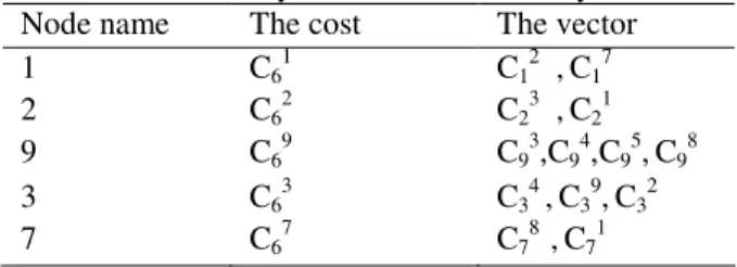
Routing Table : After the construction of the tree, each node constructs a routing table that contains information about their neighbors. The routing table consists on many rows as the number of neighbors ( at most 8) and three columns. Each row contains information about determined neighbor (child or sibling) (To distinguish the children from the sibling a labeling scheme like that proposed in [23,25] can be used here. that is out of our interest in this work). In the first column of each row is inserted the node label. The second column contains the cost of transmission on the link that end by such node. And the third columns contains the node's vector. That means, by reading the second column of the table we find the vector of the node under consideration, and by reading the table by rows we find information about the neighbors. The routing table is modified periodically given the information collected in the monitoring phase. Table.1 represents the routing table of the node (6) in the graph represented in example 1 before mobility. And Table.2, represents the routing table of the node the same node (6) after mobility.
Routing Protocol: Generally, the performance of the routing table is evaluated by the resources consumption in forwarding a packet from a given source to determined destination. In our algorithm, when a node receives a packet is not destine to it, it consults the routing table to compute the minimum cost of the path
used to forward the packet in its sub tree.That means, if two paths exist, it will be choose the economic one in term of power consumption. For example, from table.1, if the node 6 must send a packet to the node 4 in its routing tablethere are two paths with different cost C94 , C34. Based on the minimum cost, the packet will be forwarded to the node 9 or 3.
RESULTS
Analytical Results: Analyzing the equation 5, we can note that there are only two factors that influence in the power consumption in the routing of packet, are the height of the tree and the packet size. In our results, we have been analyzed the variation of the power consumption with these two factors in a network with 100 nodes divided in 2,4,5,10 clusters.
The variation of energy consumption with the network size: In our network, given a determined network size varying the number of clusters influences the size of cluster and varies also the distribution of nodes in the cluster.
Table.1: The routing table of the node 6 in the tree constructed by TDA before the mobility
Node name The cost The vector
1 C61 C12 ,C17
2 C6
2
C2 3
,C2 1
9 C69 C93,C94,C95,C98
3 C6
3
C3 4
,C3 9
,C3 2
7 C67 C78 ,C71
Table.2: The routing table of node 6 in the tree constructed by TDA after the mobility
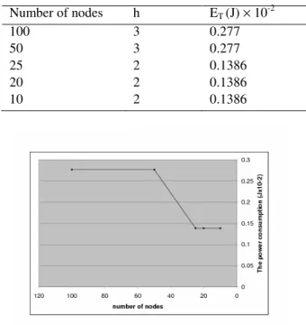
Table 3, shows the variation of power consumption with cluster size for a packet of 240 bytes. Since the tree constructed by TDA grows by width and not by height form figure 2,and table 3, we can note that for a certain number of nodes, h is the same and consecutively the power consumption is fixed , so the distribution of nodes in the manner described in TDA allows the division between the power consumption in the routing of a packet and the network size. If the number of nodes in the cluster increases from 50 to 100, ET is the same because h is the same.
Node name The cost The vector
1 C61 C12 ,C17
9 C6
9
C9 3
,C9 4
,C9 5
8 C68 C87 ,C89
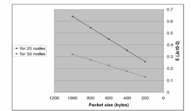
The variation of energy consumption with the packet size: The variation of the power consumption with the packet size in a network with 100 nodes divided in 2, 4 clusters is shown in table 4.
The results presented in table 4, show that the power consumption is linearly increased with the packet size. Analyzing the results presented in tables (3, 4) we can conclude that the packet size is the main factor that influences in the variation of the power consumption. However, applying our power saving mechanism in a tree constructed by TDA gives a scalable system in which the power consumption is not related to the network size. From TDA construction each node can maintain at most 5 children and the tree constructed by TDA grows with the network size by width and not by length and given the result in table 3, if the number of nodes is increased from n to 10n, the power consumption ET does not increase to 10 ET.
Table.3: Analytical results: the variation of power consumption with cluster size.
Fig. 2: the variation of ET with the network size
Table.4: Analytical results: the variation of power consumption with the packet size
Packet size (bytes) ET (J) × 10-2 ET (J) × 10-2
200 0.258 0.129
400 0.354 0.177
600 0.45 0.225
800 0.546 0.273
1000 0.642 0.321
Table.5: Analytical Results : The variation of power consumption with the number of hops
Number of hops
2 3 5 6
ET (J) × 10-2
0.1386 0.2772 0.5544 0.6930
Table 5, show the variation of power consumption in packet forwarding given the varying of number of hops. where we varied the number of hops traveled by a packet of 240 bytes considering that each hop corresponds to a level in the tree. The power consumption is increased linearly with the packet size (Fig .3).
Simulation results : All our simulations were run on top of NS-2.28, in which the system is represented by a set of mobile NS nodes distributed in clusters connected to each other by bidirectional wireless links. Our algorithm can run on top of existing routing protocols for ad-hoc networks (AODV-DSDV). The MAC protocol used was IEEE 802.11 with bandwidth 1M.B and radio propagation was modeled as two ray ground with unidirectional antennas. The antennas were centered in the node and 1.5 m ahead of the node that means x=0, y=0, z=1.5. The topology is a flat grid. Different simulations were performed, varying the number of nodes in the cluster with different topology size (720 ×1200- 1600×1200). At the beginning of the
simulation, each node had energy of 0.010 J and the minimum delay was 50us. The share media interfaces were initialized to make them work like 9.4 MHZ Lucent Wave LANDSS Radio interface. Receiving power was 0.3 mw and transmitting power 0.6 mw. During the simulation
Table 6: The variation of power consumption with packet size in the case of sending
Packet size
(bytes)
220 272 280 292
ET (J) × 10-2
for 10 nodes
0.8904 - - 0.9763
ET (J) × 10-2
for 20 nodes
- 0.7375 - 0.9763
ET (J) × 10-2
for 30 nodes
- 0.7375 - 0.71986
ET (J) × 10 -2
for 50 nodes
- 0.7375 0.8003 -
time, each node changed its energy given its state. When a node starts discovering its neighbors, it sends a broadcast message and sets its initial energy. Then, it waits to receive a response message ( the node Number of nodes h ET (J) × 10-2
100 3 0.277
50 3 0.277
25 2 0.1386
20 2 0.1386
consumes energy during the waiting time). During the simulation time each node sends only one broadcast message. However, it receives more than one response message.
The variation of power consumption with packet size: Different simulations were done, with different network sizes (10,15,20,30,50 nodes) we have been analyzed the variation of the power consumption with the packet size in the case of sending and receiving. Tables (6,7) show that the power consumption is linearly increased with the packet size in case of sending and receiving respectively in different network sizes. Figure.4, shows the variation of the power consumption for sending a packet in networks with 50,30 nodes. We can note
that the power consumption is increased with the packet size. From column 3 in tables(6,7), we can conclude that the power consumed for sending and receiving a packet is not related to the network size.
The variation of power consumption with the number of hops: Our simulation results indicate that the number of hops traveled by a packet from a given source to a given destination is an important factor that influences the power consumption in the network. Columns 2,3 of table 8 show that the power consumption for routing a packet of 240 bytes in a network of 30 nodes from a given source to a certain destination is twofold when the packet travel two hops instead one.
Figure.5 shows that the power consumption is increased linearly with the number of hops in the transmission of a packet of 240 bytes. The data presented in table 8 , indicate that the power consumption in our system is independent of the network size and that agrees with our theoretical results (equation 5).
Fig. 3: Analytical Results: the variation of ET with the packet
size
Results analysis: Our analytical results are confirmed by our simulation results. From figure.2 and table.3 we can see that the power consumption in forwarding a packet of 240 bytes in a network of 10,20,25 nodes is fixed because the height of the tree is the same this result is confirmed by the simulation where reading the third column in table 6 we note that the power consumption in a network of 20, 30 nodes is invariable in sending a packet of 240 bytes. That means, the power consumption in the case of sending and receiving the same packet is fixed with the variation of the network size (10,20,30). Analyzing equation 5, we can conclude that the power consumption in forwarding a packet in our system is influenced by only two factors are the packet size and the number of hops. Reading the table.6 by rows we can denote that the power consumption is increased linearly with the packet size (figure.3). however, in our simulation results(figure4) the power consumption is increased with the packet size.
Comparing tables 5,8 we can conclude that the power consumption is linearly increased with the number of hops. Our simulation results give a very similar values to that expected in the analytical analysis(specially for 2 and 3 hops).
Related works : Power control techniques are used in wireless communication to reduce interference and to conserve energy. This strategy has particularly interesting applications in a multihop MANET network, because the transmission power required for the communication between two nodes is increased exponentially with their distance, and the total power required to transmit a packet via multihop may be less than the energy required to transmit it directly.
In the literature, the power saving problem is studied widely, there are two main problems raised in that context the first is the Minimum Energy Consumption Broadcast Sub graph problem (MECBS), that is the problem of finding a minimum transmission range in MANET network that, corresponds to a spanning tree with minimum total cost of transmission. This problem is proved in [3], to be NP-hard to approximate with logarithmic factor. While it remains NP-hard even if considering geometric 2-dimension network[4]. The second problem is the topology control problem that is the problem of finding a set of transmission ranges that gives a minimum power topology while maintaining the network connectivity[12].
Power Algorithm ). The idea on which BIP is based is the construction of a minimum energy tree rooted at a given source node, that reaches all the desired destinations. It is proposed for wireless networks with fixed node locations. BIP works as follow: first, it determines the nearest neighbors with minimum expenditure power to the source node, constructing in that the source tree. Then, it adds to that tree the nodes with minimum additional cost (Minimum cost is an incremental cost that allows a node by increasing its power to reach additional nodes).
For each of the three previous nodes ( source, neighbor, nodes reachable by incremental cost) is determined cost to reach new nodes. BIP is similar to Prim's algorithm [5], for the formation of the Minimum Spanning Tree (MST's), in the sense that the new nodes are added to the tree one at time until all nodes are included in the tree. The main difference between the two algorithms is that in Prim's algorithm, the link costs remains unchanged throughout the execution of the algorithm. However, in BIP the link cost must be updated dynamically at each step.
The best heuristic algorithm to MECBS problem appears to be the one based on the construction of an Euclidean Minimum Spanning Tree rooted at the source. This algorithm is denoted as MST-ALG, this heuristic runs in polynomial time and always returns a feasible solution. The best experimental results is achieved in [21]
.
In[3], a comparison of the cost of MST-Alg solution to lower bound of the relative optimum, is done. First, the lower bound (that is not the directed lower bound yielded by the approximation ratio) is computed on the optimal cost of any instance of the problem. Then, this lower bound in order to evaluate the approximation ratio over several thousands of random instances. The results show that the approximation ratio for all the random instances has never achieved a value greater than 6.4. The above lower bound is exploited on the optimal establishes a direct connection between the approximation ratio of the MST based solution and the ratio C(s)(where C(s)is the cost of the MST of a set of nodes s on the plan and the minimum area that contains s). This approximation ratio to MST-ALG is not larger than 4.C(s).
In [14], is studied two fundamental problems related to energy saving are: the minimum energy broadcast tree problem and the minimum energy multicast tree problem. The two problems concentrating on constructing a tree in which the broadcast/multicast of a
message from a source node to all other nodes is done in a manner that the summation of the transmission powers at all nodes in the path is minimized. In [14], is demonstrated that minimum energy multicast tree problem is NP complete by reducing the Steiner tree problem to it. Then, an approximate algorithm for the problem in general setting is presented, that delivers an approximate solution with a bounded performance guarantee. For the special case, where all the nodes have the same type of battery, an approximation algorithm with better performance ratio is presented, compared with its general counterpart. In addition, for the minimum energy broadcast tree problem an approximation algorithm is presented where the total transmission power needed for maintaining the broadcast tree is O(log3n) times of the optimum, and the complexity of the proposed algorithm is O( k n2 log n) wherek is the number of power levels at each node in the wireless network. The technique used to obtain the previous results is extended to solve theminimum energy multicast tree problem to which is found an approximation algorithm in which the total transmission power consumed of themulticast tree is O(log3|D|) time of the optimum, where D is a set of terminal nodes. The time complexity of the proposed algorithm is O(kn|D|log|D|).
In [19], is proposed an algorithm for constructing a subgraph Gmin of the maximum energy path preserving graph.
of [19], is that in the work presented in [19] a node broadcast a single neighbor discovery message at pmax reducing in that the number of replies. The algorithm proposed by Li in [13], performs well in the dense networks because a node does not need to transmit at pmax to find its neighbor set. While, in moderately populated networks it tends to exhibit poor performance because each node must transmit with pmax to search its neighbor set.
There are a set of protocols based on dominating set proposed for power saving [2,22], Span is one of them [2], in which a group of nodes called coordinators form a connected dominating set over the network, these nodes do not sleep and forward packets, acting as low latency routing backbone for the network. Non coordinator nodes follow a synchronized sleep/wake cycle, exchanging traffic using an algorithm based on the beaconing and traffic announcement method of IEEE 802.11 IBSS power saving (In IEEE 802.11 IBSS power saving, a synchronized beacon interval is established by the stations. All stations wake up at the beginning of the beacon interval and remain awake until the end of the ATM windows (Ad-Hoc Traffic Identification Message). Once the synchronization beacons has been transmitted, each station sends an ATM to every other station for which it has pending unicast traffic. Each station that receives such ATM, responds with an acknowledgment at the end of the ATM windows. Stations that have not sent or received ATM go back to sleep). Span is intended to maximize the amount of times nodes spend in sleep state, while minimizing the impact of management on latency and capacity.
Topology control in wireless network depends on uncontrollable factors such as transmission power and antenna direction. Topology control is important because a wrong topology can reduce the capacity, increases the end-to-end packet delay and decreases the robustness to node failures. If the topology is too sparse, the network may become partitioned, and the end-to-end delay becomes high. On the other hand, If the topology is too dense, the limited spatial reuse reduces network capacity. In [12], three algorithms for power control and routing in clustering are proposed. The first is ClusterPow is based on the construction of a cluster with the same power level pi. The second algorithm is Tunneled ClusterPow, that works in a manner to reduce the power consumption using a recursive look up only on the destination node. The third algorithm is MINPOW, whose basic idea is not new: it provides an optimal routing solution with respect to the total power consumed in the communication.
In [9], is proposed power aware routing optimization protocol (PARO) that chooses a path that minimizes the total transmission power consumed by all nodes on the path. PARO has three core algorithms which are: overhearing algorithm ,that handles packets received from neighbors and creates an entry in the overhear table, or refreshes the entry if the neighbor already exists. The second algorithm is the redirection algorithm , that performs the route optimization that means find the path that requires less transmission power. The third algorithm is the route maintenance algorithm, in which the source node transmits route maintenance packets to destination whenever there is no data packet to send for a fixed time interval.
CONCLUSION
In this paper we have been proposed a mechanism for the power saving that help in the routing process. The idea is to organize the network in a dynamic tree in which the communication is done by levels given the transmission range. Our goal was the construction of a topology that can be an infrastructure to different Ad-Hoc application, that consumes less energy as possible. We have obtained a scalable system in which the power consumption is independent of the network size and is depend only on two main factors are the packet size and the number of hops traveled in the tree.
The main contribution in this paper is to limit the number of children for each root to reduce the interference effects and to make the tree grows by width not by height of the tree, that reduce the power consumption. Our mechanism for power saving in this tree is that each node adjusts its transmission range to be reachable only by their well defined neighbors saving in that a power in the transmission to reach undesiderable nodes. A little saving in the power consumption in each node may results in a total power saving in all the network that increase the system life time
Table7: The variation of power consumption with packet size in the case of receiving
Packet size
(bytes)
220 240 260 280
ET (J) × 10-2 for
10 nodes
- 0.2920 - 0.2675
ET (J) × 10-2 for
20 nodes
0.2968 0.2920 - -
ET (J) × 10-2 for
30 nodes
- 0.2920 - -
ET (J) × 10-2 for
50 nodes
Fig.4: The variation of energy with packet size
Table.8: The variation of power consumption with the number of hops
Network size 30 30 50 50
# of hops 1 2 2 3
ET (J) × 10-2 0.0701 0.14 0.145 0.215
Fig.5: The variation of energy with the number of hops
REFERENCES
1. Luiz Albini, Antonio Caruso, Stefano Chessa, Piero Maestrini, 2004. Reliable Routing in Wireless Ad-Hoc Networks. Technical Report 2004-TR-o8. CNR.ISTI.PI.3-9.
2. B.Chen, K.Jamieson, M.Balakrish and R.Morris, 2001. Span: An energy Efficient Coordination Algorithm for Topology Maintenance in Ad-Hoc Wireless Networks. In Proceedings of the 17th Annual International Conference on Mobile Computing and Networking, PP:85-96.
3. A. Clementi, G. Huiban, P. Penna, and Y.C.Vehoeven, 2002. On the approximation Ratio of the MST-based Heuristic for the Energy-Efficient Broadcast Problem in static Ad-hoc Radio Networks. In. Proc of the 1st Workshop on wireless Mobile Ad-hoc Networks WMAN 2002. 4. A. Clementi, P. Crescenzi, P. Penna, G. Rossi, and
P. Vocca, 2001. On the Complexity of Computing Minimum Energy Consumption Broadcast Sub graphs. In Proc of STACS, LNCS 2010, PP: 121-131.
5. Thomas H. Cormen, Charles E. Leiserson, Ronald L. Rivest, and Clifford Stein, 2001. Introduction to Algorithms. Second Edition. MIT Press and McGraw- Hill.. pp.567-574 .
6. Budhaditya Deb, Sudeept Bhatnagar and Badri Nath ,2002. A Topology Discovering Algorithm For Sensor Networks with Applications to Network Management. Short Paper in IEEE CAS Workshop September 2002.
7. Laura Marie Feeney, Martin Nilsson, 2001. Investigating of the Energy Consumption of a Wireless Network Interfaces in Ad-Hoc Networking Environment. In IEEE 20th INFOCOM. vol:3. Archorage AK. PP:1548-1557. April 2001.
8. J.Guha and S. Khuller, 1998. Approximation Algorithms for Connected Dominating Sets. Algorithmica, 20(4). PP: 374-387.
9. J. Gomez, A.T Campbell, M. Naghshineh, and C. Bisdikian, 2003. PAO: Supporting Dynamic Power Controlled Routing in wireless Ad-Hoc Networks. ACM/KLUWER journal on Wireless Networks (WINET). vol 9, PP:443-460. September 2003. 10. D.B. Johnson, D.A. Maltz and Y.C.Hu. The
Dynamic Source Routing Protocol for Mobile Ad-Hoc Networks (DSR). IETF Internet draft, version 9.
11. David B. Johnson and David A. Maltz, 1996. Dynamic Source Routing in Ad-Hoc Wireless Networks. In Imielinski and Korth editors, Mobile Computing, Volume 353.Kluwer Academic Publishers.
12. V. Kawadia and P.R. Kumar, 2003. Power Control and Clustering in Ad-hoc Networks. In Proceedings of the IEEE INFOCOM Conference, PP:459-496.
15. Charles Perkins and P. Bhagwat, 1994. Highly Dynamic Destination-Sequenced Distance Vector Routing (DSDV) for Mobile Computers. In ACM SIG- COMM'94: Conference on Communications Architectures Protocols and Applications. PP: 234-244.
16. C. Perkins and E. M. Royer, 1999. Ad-Hoc on Demand Distance Vector Routing (AODV). In IEEE WMSCA 99. PP:90-100. 1.
17. Ravi Prakash, Roberto Baldoni, 1998. Architecture for Group Communication in Mobile Systems. Proceeding of the 17th IEEE Symposium on Reliable Distributed Systems(SRDS). October 20-23.1998. PP:235- 241.
18. Ram Ramanathan, Regina Rosales-Hain, 2000. Topology control of Multihop wireless Networks using Transmit Power Adjustment.
19. Ashikur Rahman, Pawel Gburzynski, 2005.On Constructing Minimum Energy Path Preserving Graphs for Ad-Hoc Wireless Networks. In Proceedings of the IEEE International Conference On communications. ICC 2005. May 16-20. Seoul-Korea .
20. V.R.Syrotiuk, S.Bassagni, I. Chlamtac and
B.A.Woodward,1998. A Distance Routing Effect Algorithm for Mobility (DREAM).In ACM/IEEE MOBICOM 98.PP:76-84.
21. Jeffrey E. Wieselthier, Gam D. Nguyen, Anthony Ephremides, 2000. On the Construction of Energy efficient Broadcast and Multicast trees in wireless Networks. In Proceedings of the 19th Annual Joint conference of the IEEE Computer and Communications Societies (INFCOM), PP:585-594.
22. J. Wu, M. Gao and I. Stojmenovic, 2001. On Calculating Power Aware Connected dominating Seta for Efficient routing in Ad-Hoc Wireless Networks .In Proc of the IEEE International conference on Parallel Processing. PP:346-353. Sep 2001.
23. Arwa Zabian, Maurizio A. Bonuccelli, 2004. On the Latency of BFS Based Internet Cooperative Web Caching. IEEE. In Proceedings of the 1st International Conference on Information Communication Technologies: from Theory to Applications. ICTTA'04. 19-23 Aprile. PP:637-638. Damasco-Syria.
24. Arwa Zabian, Maurizio Bonuccelli, 2005. Topology Discovering Algorithm for Mobile Wireless Networks. the 7IFIP International Conference on Mobile and Wireless communications Networks (MWCN'05). September 2005.