www.nat-hazards-earth-syst-sci.net/14/2053/2014/ doi:10.5194/nhess-14-2053-2014
© Author(s) 2014. CC Attribution 3.0 License.
Extreme storm surges: a comparative study of frequency analysis
approaches
Y. Hamdi1,2, L. Bardet1, C.-M. Duluc1, and V. Rebour1
1Institute for Radiological Protection and Nuclear Safety, BP17, 92 262 Fontenay aux Roses CEDEX, France 2National Engineering School of Gabes, University of Gabes, Rue Omar Ibn-Elkhattab 6029, Gabès, Tunisia
Correspondence to: Y. Hamdi (yasser.hamdi@irsn.fr)
Received: 30 September 2013 – Published in Nat. Hazards Earth Syst. Sci. Discuss.: 19 November 2013 Revised: 13 May 2014 – Accepted: 14 May 2014 – Published: 13 August 2014
Abstract. In France, nuclear facilities were designed around
very low probabilities of failure. Nevertheless, some ex-treme climatic events have given rise to exceptional observed surges (outliers) much larger than other observations, and have clearly illustrated the potential to underestimate the extreme water levels calculated with the current statistical methods. The objective of the present work is to conduct a comparative study of three approaches to extreme value analysis, including the annual maxima (AM), the peaks-over-threshold (POT) and the r-largest order statistics (r-LOS). These methods are illustrated in a real analysis case study. All data sets were screened for outliers. Non-parametric tests for randomness, homogeneity and stationarity of time series were used. The shape and scale parameter stability plots, the mean excess residual life plot and the stability of the standard errors of return levels were used to select optimal thresh-olds and r values for the POT andr-LOS method, respec-tively. The comparison of methods was based on (i) the un-certainty degrees, (ii) the adequacy criteria and tests, and (iii) the visual inspection. It was found that ther-LOS and POT methods have reduced the uncertainty on the distribu-tion parameters and return level estimates and have system-atically shown values of the 100 and 500-year return levels smaller than those estimated with the AM method. Results have also shown that none of the compared methods has al-lowed a good fit at the right tail of the distribution in the presence of outliers. As a perspective, the use of historical information was proposed in order to increase the represen-tativeness of outliers in data sets. Findings are of practical relevance, not only to nuclear energy operators in France, for applications in storm surge hazard analysis and flood man-agement, but also for the optimal planning and design of
fa-cilities to withstand extreme environmental conditions, with an appropriate level of risk.
1 Introduction
Nuclear power is the primary source of electricity in France and it is operated by Electricité de France (EDF). Nuclear power facilities have to be designed to withstand extreme environmental conditions. The majority of nuclear facilities in France are located away from the coasts and obtain their cooling water from rivers. Five plants are located on the At-lantic French coast: Blayais, Gravelines, Penly, Paluel, and Flamanville. Generally, safety and design rules stipulate that protection structures should be designed to exceed specific levels of reliability. This requires specification of values of design variables with very low probabilities of exceedance (considering, for instance, a 1000-year return surge). The storm surge is a random environmental component which is fundamental input to conduct a statistical investigation for the submersion hazard (e.g., Bernier and Thompson, 2006; Von Storch et al., 2008; Bardet et al., 2011; Bernardara et al., 2011; Irish et al., 2011; Northrop and Jonathan, 2011).
not designed for such a combination of events (Mattéi et al., 2001). Therefore a guide of protection including fundamen-tal changes to the evaluation of flood hazard at nuclear power plants has been recently published by the Nuclear Safety Authority (ASN, 2013). However, some issues like the fre-quency estimation of extreme surges remain among the prior-ities of the Institute for Radiological Protection and Nuclear Safety (IRSN).
Statistical modeling is essential for the estimation of such extreme events occurrence. Relating extreme events to their frequency of occurrence using probability distributions has been a common issue since the 1950s (e.g., Chow, 1953; Dal-rymple, 1960; Gringorten, 1963; Cunnane, 1978; Cunnane and Singh, 1987; Chow et al., 1988; Rao and Hamed, 2000). The frequency estimation corresponding to long return peri-ods is based on the extreme value theory (Coles, 2001).
The AM (annual maxima) method is a simple and straight-forward approach, adopted by many national design codes worldwide, in which a generalized extreme value (GEV) dis-tribution is used to fit annual maximum observations. It uses data separated into blocks of 1 year and from these blocks only the maximum is used. However, the statistical extrapo-lation, to estimate storm surges corresponding to high return periods, is seriously contaminated by sampling and model uncertainty if data are incomplete and/or available for a rela-tively limited period. Another major disadvantage of the AM is that if we only extract the annual maximum observation, we will lose lots of high sea water levels occurring during the whole year. This has motivated the development of ap-proaches to enlarge the sample extreme values beyond the annual maxima. A way around this is to use a point pro-cess method (PPM) by setting an exceedance high threshold above which observations are taken as extremes (POT ap-proach) or by extracting a fixed number of high observations in each year (r-LOS approach). This way will allow us to use much more of the data collected during the year.
The POT (peaks-over-threshold) and ther-LOS (r-largest order statistics) approaches are two particular cases of the PPM. The PPM is commonly considered as an alternative to the AM method. The POT approach models the peaks ex-ceeding a sufficiently high threshold. The generalized Pareto distribution (GPD) is the most adapted theoretical distribu-tion to fit POT series. In addidistribu-tion, the threshold leads to a sample with data which are more representative of extreme events. However, it is difficult to choose a threshold level and this makes for subjectivity in what should be taken as a rea-sonable threshold. The use of a too-low threshold introduces automatically a bias in the estimation by using observations which may not be extreme data and this violates the principle of the extreme value theory. On the other hand, the use of a too-high threshold will reduce the sample of extreme data. It was also shown in the literature that the POT approach cannot easily be used in presence of temporal and spatial variability, because a separate threshold must be selected for each year and site (Butler et al., 2007). The r-LOS model is similar
to the AM except that, instead of recording only maximum observations for each block, ther largest ones are recorded (the case withr=1 is equivalent to the AM approach). The function density for the r-LOS model is slightly different from the AM density, but it can be approximated to the AM model, considering that eachrvalue is the maximum obser-vation of a fictitious year. The r-LOS model is considered by many authors as an alternative to the more usual AM and POT methods (Smith, 1986; An and Pandey, 2007; Butler et al., 2007). The advantage of using a PPM method is that we can include more recorded observations into the estimation of the distribution function parameters and thus with more data we will decrease the estimation variance and be more confident about our parameter estimates. The reader is re-ferred to Coles (2001) for more details about AM and the PPM methods presented above.
As it has been outlined with the storms of 1987, 1999 or 2010, data sets may contain outliers. Traditionally, an out-lier is defined as an observation point that departs signifi-cantly from the trend of the remaining observations when displayed as an experimental probability scatter plot. Con-sequently, outliers interfere with the fitting of simple trend curves to the data and, unless properly accounted for, are likely to cause simple fitted trend curves to grossly misrep-resent the data. It was shown in the literature that the meth-ods outlined above (MA and PPM) are not always adapted to data sets containing outliers (e.g., Stedinger, 1988). In an earlier study to overcome the shortcoming of short data se-ries and the outlier issue, Bardet et al. (2011) and Bernardara et al. (2011) assessed POT series of storm surges in a re-gional frequency analysis framework. In a rere-gional context and in comparison with local analyses, observed exceptional surges become normal extreme values and do not appear to be outliers any more. However, the regional frequency anal-yses, in particular the inter-site dependency issue, need to be improved (Bardet et al., 2011).
A brief review of the theoretical background of the ex-treme value frequency analysis is presented in Sect. 2 of this paper. The AM,r-LOS, and POT methods applied to storm surges data collected at 21 sites in the French Atlantic coast are presented in Sect. 3, with a verification of the frequency analysis assumptions. Section 4 summarizes the discussion as well as a comparison of the AM, r-LOS and POT ap-proaches. Further discussions on using historical information to improve the frequency estimation of extreme surges are presented in Sect. 5, before the conclusion and perspectives in Sect. 6.
2 Extreme value frequency estimation
Regardless of the analysis method, a standard frequency es-timation procedure includes the following steps: (i) verifica-tion of randomness, homogeneity and staverifica-tionarity hypothe-ses and detection of outliers; (ii) computation of empirical probabilities of exceedance using sorted and ranked observa-tions; (iii) fitting a curve to these observations with distribu-tion funcdistribu-tions, parameters estimadistribu-tion and applying adequacy criteria and tests to select the more appropriate method and the best distribution to represent the data; (iv) extrapolating or interpolating so that the return period T of the extreme value of interest (say 100 years) is estimated.
2.1 Hypotheses and statistical tests
Randomness, homogeneity and stationarity of time series are necessary conditions to conduct a frequency analysis (Rao and Hamed, 2001). Three non-parametric tests were used: the Wald–Wolfowitz test (WWT) for randomness (Wald and Wolfowitz, 1943), the Wilcoxon test (WT) for homogene-ity (Wilcoxon, 1945) and the Kendall test (KT) for stationar-ity (Mann, 1945). Another important test but not required to conduct a frequency analysis is the Grubbs–Beck test (GBT) for the detection of outliers (Grubbs and Beck, 1972).
2.2 Frequency estimation
Several formulas exist to calculate the empirical probabil-ity of an event. On the basis of different statistical criteria it is found in several studies (e.g., Alam and Matin, 2005; Makkonen, 2006) that the Weibull plotting position formula pe=m/ (N+1)directly follows from the definition of the return period (mis the rank order of the ordered surges mag-nitudes andN is the record length). It was also shown that this formula (Weibull, 1939) predicts much shorter return periods of extreme events than the other commonly used methods. The Weibull plotting position was then used in the present work.
Of the many statistical distributions commonly used for extremes, the GEV function was retained for the AM andr -LOS methods and the GPD function was used to apply the POT approach.
The GEV distribution introduced by Jenkinson (1955) is the limiting distribution for the maximum (and the mini-mum) of i.i.d. (independent and identically distributed) ran-dom variables. It combines three asymptotic extreme value distributions, identified by Fisher and Tippet (1928), into a single form with the following cumulative distribution func-tionF:
F (x)=
e−
1+ξx−σµ−1/ξ
ξ 6=0 e−e−(x−µ)/σ ξ =0
, (1)
whereµ,σ >0, andξ are the location, scale, and shape pa-rameters, respectively. The parameterization for the shape parameter ξ in Eq. (1) follows the notational convention prevalent today in the statistics literature; for example, in the hydrologic literature, it is still common to parameterize in terms ofξ∗= −ξ instead.
Depending on the value of the shape parameter ξ, the GEV can take the form of the Gumbel, Fréchet or Nega-tive Weibull distributions. Whenξ=0, it is the Type I GEV (Gumbel) distribution which has an exponential tail. When ξ >0, the GEV becomes the Type II (Fréchet) distribution. In the third case, whenξ <0, it is the Type III GEV (the re-verse Weibull function). The last one has a finite and short theoretical upper tail(∞< x < µ−σ/ξ )that may be use-ful for estimates of specific cases of extreme values such as surges, which may have an upper bound. The heavy upper tail in the first case with the Fréchet distribution is unbounded (µ−σ/ξ < x <∞)and allows for relatively high probabil-ity of extreme values. Generally when examining extreme storm surge events we are interested in asking the question: How often do we expect a region to be submerged by sea water? And if it is submerged how high will the surge be? To answer this question, we need to calculate theT years return level. The 1/preturn levelzˆp(computed from the GEV
dis-tribution) is the quantile of probability(1−p)to exceedzˆp
and it is given by
ˆ zp=
( ˆ µ−σˆˆ
ξ n
1−yp− ˆξ o
ξ6=0 ˆ
µ− ˆσlog yp ξ=0
, (2)
whereyp= −log(1−p)andµˆ,σˆ andξˆ are the GEV
dis-tribution parameters estimated with the maximum likelihood method.
On the other hand, as mentioned earlier, a GP distribution calculates probabilities of observing extreme events which are above a sufficiently high threshold. Given a thresholdu, the distribution of excess values ofx overuis defined by
Fu(y)=Pr{X−u≤x|X > u} =
F (x)−F (u)
1−F (u) , (3)
when the selected thresholduis sufficiently high, the asymp-totic form of the distribution function of excessFu(y)
con-verges to a GP function (e.g., Pickands, 1975) which has the following cumulative distribution function:
G (x)= (
1−(1+ξ x/σ )−1ξ ξ 6=0
1−e−x/σ ξ =0 . (4)
The GP distribution corresponds to a (shifted) exponential distribution with a medium-size tail when ξ=0, and to a long-tailed (and unbounded) ordinary Pareto distribution for positive values of ξ and finally, when ξ <0, it takes the form of a Pareto Type II distribution with a short tail upper bounded byµ+σ/ξ.
Several methods exist to estimate distribution parameters. Although for most of the distribution functions, the maxi-mum likelihood method is considered in many investigations as an excellent option for parameter estimation, it has been shown that the method of moments is more effective (Ashkar and Ouarda, 1996) when using the GPD. For both the GEV and the GP distributions, the parameters were estimated in the present work with the maximum likelihood method.
2.3 Adequacy criteria and tests
Questions like the adequacy in the statistical analysis and goodness-of-fit (GOF) tests should be addressed when com-paring different distributions and methods. Many GOF tests studies were conducted in the literature. Steele and Chaseling (2006) have shown that no single test statistic can be recom-mended as the “best” and we need to consider carefully the choice of a test statistic to optimize the power of our test of goodness of fit. Conventional measures of the adequacy of a specified distribution and to compare and select the more appropriate method is to compute the BIAS and RMSE (root mean squared error). The RMSE, also known as the fit stan-dard error, is the square root of the variance of the residuals. It indicates the absolute fit of the model to the data and how close the observed probabilities are to those of the model. As the square root of a variance, RMSE can be interpreted as the standard deviation of the unexplained variance, and has the useful property of being in the same units as the response variable. Lower values of RMSE indicate better fit. RMSE is a good measure of how accurately the model predicts a response. The Akaike and the Bayesian information criteria are two other selection criteria based on the likelihood func-tion and involving the number of parameters and the sample size. Since the methods that we compare in the present pa-per produce data sets of different lengths and use the same distribution function, our comparative study will be biased if we use these two last criteria (because they are based on the sample size).
In addition to these criteria, many adequacy statistics and goodness-of-fit tests, such as the Chi-2, the Kolmogorov– Smirnov (KS) and the Anderson–Darling (AD), can also be
used to discriminate between distributions and/or methods. The Chi-2 test can be used to verify the hypothesis about the parent distribution of the sample. The advantage of this test is that one can be certain that a fit is not adequate if this test fails for a distribution. On the other hand, this test has the shortcoming of being considered, by the scientific commu-nity, not very powerful. Moreover, we strongly believe that using the Chi-2 for continuous distributions is a bad idea (the test result depends strongly on the choice of the classes far more than the values of the sample). The AD test (Stephens, 1974) is used to test if a sample came from a population with a specific distribution. It is an improved version of the KS test and gives more weight to the distribution tails than do the KS and the Chi-2 tests. Contrarily to the AD test, with the KS test the critical values do not depend on the specific distribution being tested. The AD test makes use of the specific distri-bution in calculating critical values and it is not distridistri-bution free. The AD test is then considered in the present paper as an alternative to the KS and Chi-2 GOF tests.
3 Study area and extraction of extreme events
time series have not been exploited) which may have a nega-tive impact on the performance of the method.
The record length was the main criterion to select the sta-tions. The AM approach was applied to sufficiently long data sets (e.g., Dunkerque, Le Conquet, Brest). We also included sites with 14 to 25-year data sets (St-Nazaire, Olonne, La Rochelle, Port Bloc) to examine the contribution of PP ap-proaches (POT andr-LOS) expanding relatively short series. Within this selected subset, some stations were lacking data for relatively long periods. In some cases, these missing peri-ods can reach several months and may occur during the sea-son of high surges (autumn and winter). This may limit the performance of AM andr-LOS frequency analysis methods. Using these criteria, a first selection was done on the annual maximum data sets. Saint-Malo, Concarneau, Le Crouesty, and Arcachon stations were removed because they have very small record lengths. Within the selected subset of AM ob-servations, the minimum length of record is 14 years (La Rochelle) and the maximum is 56 years for Brest tide gauge. Figure 1 shows record lengths of the retained sites.
3.1 Extraction of extreme events using ther-LOS and POT models
Similarly to the AM data sets, POT, andr-LOS observations were extracted from the same time series. The extraction of these data sets requires caution regarding base surges or thresholds u (for the POT approach) and r (for the r-LOS approach) values to be used. There is a bias–variance trade-off associated with these parameters. A large value ofuor a small value of r can result in large variance, but the op-posite is likely to cause a bias and violate the assumption of the Poisson process generating the extreme values (Smith, 1986). One of the criteria used to select uor r is that they minimize the variance associated with a required quantile es-timate. Coles (2001) has shown that stability plots constitute a graphical tool for selecting optimal value ofuorr. The sta-bility plots are the estimates of the GPD parameters and the mean residual life-plot as function ofuwhen using the POT approach, and the standard errors of the GEV shape parame-ter and theT years return levels as function ofrin ther-LOS case. The value should be extracted from the linear part of the curve. To avoid violating the assumption of the Poisson process generating the extreme values, the required thresh-old should be as high as possible and the required value ofr should be as low as possible (without considerably increas-ing the variance). This is why in seekincreas-ing the stability zones we begin exploring the POT diagnostic plots from the right (ushould be as high as possible) and ther-LOS ones from the left (r should be as low as possible). At the same time, to minimize the variance, the smallest value of the identified stable part is commonly considered by the scientific commu-nity as an optimal choice of u orr. It is important to note that depending on the objectives of the study, another value can be selected as long as it remains in the stable part of the
curve. The table presented in Fig. 1 shows the optimal values ofrandufor each considered site.
In ther-LOS model, a data set was extracted for each site from the raw data and the analysis was repeated forr=1–10 (ifr=1 then this simplifies to the AM method). The three GEV parameters and associated standard errors were calcu-lated. As an example, the standard errors corresponding to the shape parameter and associated with 100 and 500-year surges for the Brest (56-year data set) and Boulogne (20-year data set) sites are shown in Fig. 2. We can clearly see a decrease of the variability with an increase inrup to 3 for Brest and up to 5 for Boulogne, but there is no appreciable change in the standard error forr greater than these values. Therefore, an optimum choice ofr is expected to be close to 3 for Brest and 5 for Boulogne. As it will be presented later, the values ofrpresented in Fig. 1 are sufficient to pro-vide minimum variance quantile estimates. These values are similar to those recommended by several authors (e.g., Tawn, 1988; Guedes Soares and Scotto, 2004), who concluded that results of ther-LOS method forr=3–7 are very stable and consistent.
In the POT model, a data set was also extracted for each site from the raw data and the analysis was repeated for u=20–80 cm. To determine the required threshold, diagnos-tic plots which plot the GPD shape and modified scale pa-rameters and also the mean residual life plot over a range of threshold values were used. Figure 3 shows the mean resid-ual life plot for the Calais and Dieppe surge data sets. In-terpretation of a mean residual life plot is not always simple in practice. The idea is to find the lowest threshold where the plot is nearly linear and appears as a straight line for higher values, taking into account the 95 % confidence lim-its. For the Calais site, the graph appears to curve from u=20 cm to u=46 cm, beyond which it is nearly linear untilu=80 cm. It is tempting to conclude that there is no stability until u=46 cm, after which there is approximate linearity. This suggests we takeu=46 cm. There are 84 ex-ceedances of this threshold, enough to make meaningful in-ferences. By the same reasoning for the Dieppe data set, we can see that the plot appears roughly linear from about u≈52 cm to u≈65 cm and is erratic above 65 cm, so we selected 52 cm as a plausible choice of threshold and there are 75 exceedances of this threshold.
The second procedure for threshold selection is to estimate the model at a range of thresholds. Above a leveluat which the asymptotic motivation for the GPD is valid, estimates of the shape parameter should be approximately constant, while estimates of the modified scale parameter should be linear in u. The reader is referred to Coles (2001) for more details about modeling threshold excesses and threshold selection. We can draw the same conclusions with respect to the thresh-old value (for Calais and Dieppe sites) by inspecting the GPD modified scale and shape parameters plots presented in Fig. 3. The number of surge eventsNuis, as expected, greater
Figure 1. To the left: location of sites. In the middle: a table containing the site names and periods of records, the record lengths and the
Grubbs–Beck statistic (GBT) of each site and for the annual maxima (AM), the peaks-over-threshold (POT) and ther-largest order statistics (r-LOS) methods. Ther(ther-largest observations) andu(threshold – cm) values are also presented in this table. To the right: distribution of record lengths.
Figure 2. Estimation ofr(ther-largest observations): the GEV shape parameter and 100 and 500-year storm surges (cm) with 95 % confi-dence intervals (Brest and Boulogne sites).
Society of Civil Engineers ASCE (1949) recommended that the base surge should be selected so thatNuis greater than N, but that there should not be more than three or four events above the threshold in any one year. The CETMEF (2013) in
Figure 3. Estimation ofu(threshold – cm): the GPD modified scale and shape parameters and mean excess life plot with 95 % confidence intervals (Calais and Dieppe sites).
surges used in the present study are similar to those recom-mended by the UK Flood Studies Report (Natural Environ-ment Research Council, 1975). This range of values of Nu
was recommended by the US Geological Survey (Dalrym-ple, 1960), Tavares and da Silva (1983) and Jayasuriya and Mein (1985) as well.
3.2 Screening for outliers
Working with events in an extreme environmental conditions context requires caution about the input data. The French At-lantic sea level data sets were never screened for the numer-ical detection of outliers. The GBT was applied on series of log-transformed extreme storm surges for all stations within the selected subset. The GBT is based on the difference of the mean of the sample and the most extreme data consid-ering the standard deviation (Grubbs and Beck, 1972). Un-der the hypothesis that the logarithm of the sample is nor-mally distributed, the GBT, with a significance level equal to 5 %, highlights the extreme events with very low proba-bilities of occurrence. The table presented in Fig. 1 shows, for each site, the GBT statistic for the MA,r-LOS, and POT data sets. Sites for which the GB-statistic exceeded the one-sided critical point for GBT have experienced outliers (writ-ten with bold characters). Seven po(writ-tential outliers at seven different sites (Boulogne, Dieppe, Le Havre, Cherbourg, Le Conquet, Brest, and La Rochelle) were identified in the case of AM data sets. Three additional outliers at three differ-ent sites (Roscoff, St-Nazaire, and Bayonne) were detected when ther-LOS approach is used. Four other potential out-liers at four additional sites (Dunkerque, Olonne, Port Bloc, and St-Jean) were detected by the GBT applied on the POT series. The analysis of climatic conditions on the day the
out-lier took place shows that there is no evidence of unrealistic storm surges (storms of 1953, 1969, 1979, 1987, 1999, and 2010), all the detected outliers have been considered as cred-ible and as a result, we kept all of them in the present study.
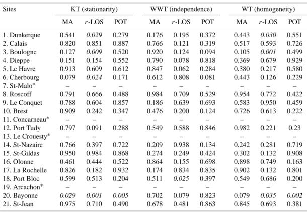
3.3 Randomness, stationarity and homogeneity tests
The record length was the first criterion to select the stations. As a second prerequisite for frequency analysis, all the time series of extreme storm surges (AM, POT, andr-LOS) must be homogeneous, stationary and independent. Table 1 shows the KT (for stationarity), the WWT (for independency) and the Wilcoxen (for homogeneity) statistics for AM,r-LOS, and POT data sets. Stations that failed these tests at signifi-cance levels of 5 % are highlighted in the Table 1 (the corre-spondingpvalues are italicised). Bayonne station failed the KT with apvalue equal to 0.029, showing a possible trend in the AM data set. Dunkerque, Boulogne, and Bayonne sta-tions failed the KT and WT with ther-LOS peaks. For the same type of data (r-LOS), the Cherbourg station failed the KT (pvalue=0.024). On the other hand, Bayonne station failed the KT and the WT with the POT data set. For all the approaches, only Port-Bloc station failed the WWT (for in-dependency) when using ther-LOS data.
Table 1. Stationarity, independence and homogeneity tests (pvalue).
Sites KT (stationarity) WWT (independence) WT (homogeneity)
MA r-LOS POT MA r-LOS POT MA r-LOS POT
1. Dunkerque 0.541 0.029 0.279 0.176 0.195 0.372 0.443 0.030 0.551
2. Calais 0.820 0.851 0.887 0.766 0.121 0.319 0.517 0.593 0.726
3. Boulogne 0.127 0.009 0.520 0.920 0.124 0.094 0.105 0.001 0.499
4. Dieppe 0.151 0.154 0.552 0.790 0.078 0.818 0.369 0.679 0.929
5. Le Havre 0.913 0.609 0.612 0.847 0.062 0.284 0.380 0.217 0.580
6. Cherbourg 0.079 0.024 0.171 0.612 0.808 0.081 0.443 0.126 0.229
7. St-Malo∗ – – – – – – – – –
8. Roscoff 0.791 0.666 0.488 0.984 0.709 0.529 0.954 0.772 0.422
9. Le Conquet 0.788 0.604 0.857 0.186 0.639 0.693 0.583 0.950 0.459
10. Brest 0.909 0.242 0.347 0.476 0.200 0.124 0.726 0.613 0.222
11. Concarneau∗ – – – – – – – – –
12. Port Tudy 0.797 0.091 0.288 0.549 0.588 0.846 0.982 0.221 0.23
13. Le Crouesty∗ – – – – – – – – –
14. St-Nazaire 0.766 0.397 0.722 0.209 0.938 0.134 0.242 0.281 0.719
15. St-Gildas 0.950 0.984 0.868 0.274 0.249 0.424 0.302 0.132 0.908
16. Olonne 0.461 0.444 0.522 0.864 0.155 0.698 0.898 0.749 0.163
17. La Rochelle 0.826 0.182 0.932 0.174 0.834 0.835 0.902 0.132 0.801
18. Port Bloc 0.599 0.513 0.204 0.511 0.025 0.397 0.549 0.686 0.200
19. Arcachon∗ – – – – – – – – –
20. Bayonne 0.029 0.001 0.005 0.702 0.079 0.823 0.079 0.035 0.002
21. St-Jean 0.975 0.710 0.490 0.678 0.481 0.863 0.845 0.693 0.381
∗Data series are very short.
techniques to climate change. Because storm surges can ex-hibit marked periodic behavior on both annual and diurnal timescales, naturally their extremes do as well. However, such cycles in extremes have not received much attention, as the AM technique does not require their explicit modeling. The annual periodicity (seasonality) in extreme storm surges is more present and visible in the r-LOS data sets than in the POT ones, especially for large values ofr. However, as the Kendall and Spearman tests applied to the POT series did not show any statistically significant non-stationarity for all the stations, more intensive and comprehensive study is needed to foresee why these tests exhibited evidence of auto-correlations, trends or cycles in somer-LOS time series. The Dunkerque, Boulogne, Cherbourg, and Bayonne sites were then removed from the analysis.
4 Results and discussion
In this section we report the results of the AM,r-LOS and POT methods of extreme storm surge analysis applied to the French Atlantic storm surges data extracted, treated and pre-sented in the last section. There are different ways to compare these statistical approaches: (i) examination of each method’s uncertainty degree; (ii) comparative study based on return levels; (iii) comparative study based on adequacy criteria and tests; and (iv) visual examination based on diagnostic plots.
4.1 Uncertainty degree
It is possible to examine the uncertainty degrees of each method. As stated earlier, optimum values ofr anduwere estimated for each site. It is interesting to note that a model predicts the future return values well only if it produces re-turn level estimates that fit inside the confidence interval. The 1/preturn levelszˆpwere calculated using Eq. (2). A degree
of uncertainty in the estimates of a return level is closely re-lated to that of the model parameters. The variance of our return level estimates was calculated using the delta method and an asymptotic approximation to the normal distribution as follows:
var zˆp=∇ztpV∇zp, (5)
where∇zp is the vector of first derivatives ofzp and V is
the variance-covariance matrix of the estimated parameters (µ, σ, ξ ).
∇zp= ∂z
p
∂µ, ∂zp
∂σ , ∂zp
∂ξ
=D1,−ξ−11−yp−ξ,
σ ξ−21−yp−ξ−σ ξ−1yp−ξlog yp E
.
Table 2. MLEs and return levels with associated standard errors for GEV distribution using AM andr-LOS data (with optimum choice ofr) and for GPD using POT data (with optimum choice ofu).
Stations µˆ σˆ ξˆ S100(SE) S500(SE)
MLE(95% CI) SE MLE (95% CI) SE MLE (95% CI) SE
AM 75.40(69.49 : 81.32) 3.02 16.18(12.07 : 20.28) 2.10 –0.175(–0.380 : 0.030) 0.105 126.51(52.18) 136.67(80.06) Dunkerque POT – – 13.53(9.26 : 17.80) 2.18 –0.033(–0.272 : 0.207) 0.122 121.83(6.15) 140.07(10.75)
r-LOS Dunkerque station failed the KT (pvalue = 0.029) and the WT (pvalue = 0.030)
AM 61.85(56.38 : 67.33) 2.79 16.53(12.57 : 20.49) 2.02 –0.425(–0.623 : –0.226) 0.101 95.25(22.82) 97.98(29.06) Calais POT – – 17.55(13.81 : 21.30) 1.91 –0.277(–0.424 : –0.130) 0.075 91.67(5.40) 98.03(7.61) r-LOS 55.94(52.22 : 59.66) 1.90 15.72(13.11 : 18.32) 1.33 –0.323(–0.453 : –0.193) 0.070 93.57(13.79) 98.04(18.79)
AM 61.63(55.40 : 67.85) 3.17 12.80(8.11 : 17.50) 2.40 0.136(–0.162 : 0.434) 0.152 143.51(149.24) 186.74(316.90) Boulogne POT – – 10.90(7.98 : 13.83) 1.49 0.104(–0.090 : 0.299) 0.099 106.43(11.02) 137.31(22.58)
r-LOS Boulogne station failed the KT (pvalue = 0.009) and the WT (pvalue = 0.001)
AM 58.42(53.61 : 63.23) 2.45 13.00(9.27 : 16.72) 1.90 0.168(–0.073 : 0.409) 0.123 148.70(98.35) 200.95(217.07) Dieppe POT – – 10.26(6.84 : 13.67) 1.74 0.186(–0.062 : 0.433) 0.126 126.64(10.40) 171.86(23.49) r-LOS 50.22(47.64 : 52.79) 1.31 12.43(10.64 : 14.22) 0.91 0.018(–0.070 : 0.106) 0.045 109.85(17.97) 131.97(33.35)
AM 66.11(59.34 : 72.88) 3.45 19.94(15.45 : 24.44) 2.29 –0.089(–0.238 : 0.059) 0.076 141.35(89.44) 161.23(148.72) Le Havre POT – – 13.72(10.18 : 17.26) 1.81 0.090(–0.098 : 0.278) 0.096 128.31(11.82) 164.3(23.8) r-LOS 53.66(50.35 : 56.97) 1.69 16.81(14.58 : 19.03) 1.13 –0.064(–0.147 : 0.019) 0.042 120.59(23.06) 139.76(39.30)
AM 47.25(43.19 : 51.31) 2.07 11.66(9.00 : 14.33) 1.36 –0.152(–0.286 : –0.019) 0.068 85.80(26.77) 94.06(41.90) Cherbourg POT – – 7.60(5.15 : 10.04) 1.25 0.046(–0.186 : 0.277) 0.118 80.94(4.91) 96.6(9.4)
r-LOS Cherbourg station failed the KT (pvalue = 0.024)
AM 48.01(44.58 : 51.44) 1.75 9.84(7.50 : 12.18) 1.20 –0.162(–0.343 : 0.018) 0.092 79.90(18.37) 86.52(28.49) Roscoff POT – – 9.88(7.58 : 12.18) 1.17 –0.099(–0.258 : 0.060) 0.081 73.53(3.77) 82.85(6.20) r-LOS 38.63(37.16 : 40.10) 0.75 8.32(7.28 : 9.37) 0.53 –0.057(–0.162 : 0.047) 0.053 72.29(4.56) 82.14(7.81)
AM 48.58(45.32 : 51.83) 1.66 9.62(7.25 : 11.99) 1.21 0.091(—0.084 : 0.265) 0.089 103.46(35.92) 128.81(72.26) Le Conquet POT – – 8.17(6.33 : 10.00) 0.94 0.097(–0.062 : 0.255) 0.081 85.37(4.21) 107.57(8.55) r-LOS 38.13(36.93 : 39.33) 0.61 7.88(7.02 : 8.74) 0.44 0.045(—0.033 : 0.123) 0.040 78.43(4.21) 94.68(8.03)
AM 51.88(48.23 : 55.53) 1.86 12.61(9.97 : 15.24) 1.34 0.047(–0.113 : 0.206) 0.081 116.57(38.70) 142.75(74.12) Brest POT – – 9.79(7.90 : 11.68) 0.97 0.070(–0.062 : 0.202) 0.067 95.25 (3.82) 118.32(7.53) r-LOS 43.17(41.74 : 44.59) 0.73 10.03(9.02 : 11.03) 0.51 0.004(–0.060 : 0.069) 0.033 94.56(7.64) 113.19(14.30)
AM 53.95(49.30 : 58.61) 2.37 10.93(7.31 : 14.54) 1.84 –0.412(–0.775 : –0.048) 0.186 76.50(16.33) 78.44(20.95) Port Tudy POT – – 13.43(10.23 : 16.63) 1.63 –0.218(–0.388 : –0.048) 0.087 74.04(5.76) 80.73(8.52) r-LOS 40.95(38.92 : 42.97) 1.03 9.77(8.34 : 11.19) 0.73 –0.113(–0.244 : 0.018) 0.067 75.96(7.25) 84.52(11.76)
AM 68.49(63.07 : 73.91) 2.76 11.63(7.60 : 15.66) 2.06 –0.078(–0.443 : 0.288) 0.186 113.46(55.48) 125.78(93.13) St-Nazaire POT – – 17.20(13.69 : 20.71) 1.79 –0.156(–0.294 : –0.019) 0.070 96.46(8.85) 108.37(13.81) r-LOS 46.97(44.93 : 49.02) 1.04 11.68(10.18 : 13.18) 0.76 –0.011(–0.134 : 0.112) 0.063 99.43(9.92) 117.23(17.85)
AM 56.67(51.60 : 61.73) 2.59 11.75(8.09 : 15.41) 1.87 –0.144(–0.461 : 0.172) 0.161 96.16(40.55) 104.86(63.89) St-Gildas POT – – 13.47(10.26 : 16.67) 1.63 –0.087(–0.265 : 0.091) 0.091 86.07(8.57) 99.59(14.27) r-LOS 47.15(44.07 : 50.23) 1.57 12.81(10.66 : 14.95) 1.09 –0.176(–0.312 : –0.039) 0.070 87.55(14.14) 95.57(21.67)
AM 56.12(50.18 : 62.06) 3.03 11.92(7.43 : 16.42) 2.29 –0.179(–0.624 : 0.267) 0.227 93.52(48.50) 100.86(74.06) Olonne POT – – 11.90(7.77 : 16.03) 2.11 –0.13(–0.38 : 0.12) 0.127 86.26(9.34) 95.77(14.93) r-LOS 42.67(39.89 : 45.45) 1.42 11.94(9.99 : 13.89) 1.00 –0.125(–0.267 : 0.017) 0.072 84.45(13.24) 94.27(21.26)
AM 48.75(37.77 : 59.73) 5.60 20.28(12.41 : 28.15) 4.01 0.048(–0.252 : 0.348) 0.153 153.20(350.90) 195.67(673.90) La Rochelle POT – – 9.18(5.51 : 12.85) 1.87 0.238(–0.070 : 0.546) 0.157 116.86(26.04) 170.76(62.80) r-LOS 44.40(39.86 : 48.93) 2.31 13.75(10.54 : 16.95) 1.63 0.045(–0.108 : 0.199) 0.078 114.67(60.20) 142.99(115.15)
AM 50.99(43.69 : 58.29) 3.72 14.59(9.38 : 19.80) 2.66 –0.299(–0.623 : 0.025) 0.165 87.43(55.71) 92.14(77.21) Port Bloc POT – – 11.48(7.13 : 15.83) 2.22 –0.098(–0.386 : 0.191) 0.147 84.56(11.89) 95.46(19.60)
r-LOS Port Bloc station failed the WWT (pvalue = 0.025)
AM Bayonne station failed the KT (pvalue = 0.029)
Bayonne POT Bayonne station failed the KT (pvalue = 0.005) and the WT (pvalue = 0.002) r-LOS Bayonne station failed the KT (pvalue = 0.001) and the WT (pvalue = 0.035)
AM 35.98(33.14 : 38.82) 1.45 7.42(5.37 : 9.47) 1.05 –0.226(–0.477 : 0.026) 0.128 57.21(10.29) 60.76(15.11) St-Jean POT – – 9.02(7.12 : 10.92) 0.97 –0.233(–0.362 : –0.105) 0.066 52.45(2.57) 56.58(3.76) r-LOS 33.42(31.67 : 35.18) 0.90 6.53(5.29 : 7.77) 0.63 –0.150(–0.315 : 0.015) 0.084 55.10(4.93) 59.79(7.72)
distribution parameters and of 100, 500, and 1000-year re-turn levels were estimated and examined for each method and each site (Table 2). Stations that failed one or several
Figure 4. The standard error associated with 100-year (left) and 500-year (right) surges versus the value ofr(ther-largest observations) and
u(threshold).T is the return period.
likelihood estimates (MLE). The results given in Table 2 in-dicate that a systematic reduction, compared to the AM and POT methods, in the uncertainty on the parameters estima-tion when usingr-LOS approach (more confidence to param-eters estimates). Indeed, compared to its MLE, the standard errors of theµˆ parameter estimated withr-LOS time series are systematically smaller than those estimated with AM data sets. It can also be seen that the standard error of theσˆ pa-rameter is systematically smaller than those estimated with POT and AM ones. Although the parameter uncertainty is often reduced when additional data is used, several stations show otherwise. This is the case for the Calais, Le Havre, Brest, Port Tudy, St-Nazaire, St-Gildas, and St-Jean stations where the POT approach results in more data than the r -LOS method without reducing the standard error. It can be concluded that additional information is a necessary condi-tion for lowering the uncertainty and providing an improved model fit to the data. However, this does not imply that hav-ing more data will improve the model fit as more data will invalidate the asymptotic assumption. Also, contrarily to the POT method, when using ther-LOS approach, a relatively large number (depending on the value ofr) of additional ob-servations become available and it is subjective to say which of the available data is in fact extreme and which is not. In other words, the statistical gain will be better if we use fewer additional values which are really extreme (the case of the POT method with a fairly high threshold for example) instead of many more values that contain multiple observations that are not really extreme, as in the case ofr-LOS time series for high values ofr.
It can also be seen that standard errors of 50, 100, and 500-year return levels decrease significantly, compared to the AM approach, for all the sites when using ther-LOS and the POT methods. This decrease in return levels is more noticeable with the POT method than for ther-LOS method. The use of the POT and ther-LOS methods leads to tighter confidence intervals as we are more certain about the theoretical return level and habitually the decrease in return levels is caused by lighter tails of distributions and smaller shape parameter given for ther-LOS and POT data sets. This allows us to con-clude that there is a decreased probability of extreme events in the right tail of the distribution when compared to the fit given by the AM model.
The effect of considering more than a single value per year is also illustrated by Fig. 4, in which the standard errors cor-responding to both ther-LOS and POT estimates of 100 and 500-year storm surges are displayed. It can be seen that the standard errors are reduced by 3–11 times asrincreases from 1 to 5, and by 1–8 times as the thresholdudecreases from 55 to 35 cm. It is also noteworthy that these differences in stan-dard errors (whenr increases and/or udecreases), become increasingly important as the size of the data sets decreases. It is undoubtedly an advantage of using ther-LOS and POT approaches instead of the AM method only when the data set size is relatively small.
4.2 Return levels
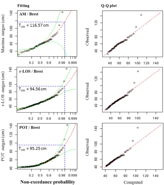
Figure 5. Visual inspection – example of a distribution fit (and Q–Q plot) for Brest station (with outlier) using AM (annual maxima),r -LOS (r-largest order statistics) and POT (peaks over threshold) methods. The 95 % lines correspond to confidence intervals. TheT100is the
100-years return period.
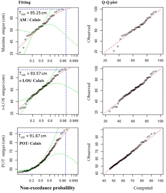
Dieppe, Brest, La Rochelle). However, theξ settings are not high enough for the theoretical curves to achieve these out-liers. None of the three approaches has allowed an acceptable closeness of fit in the upper tail of the distribution function in the presence of outliers (Fig. 5). It can be seen that the AM method has given the largest return levels and that the point process (POT andr-LOS) methods result in lower re-turn values. This increase is more noticeable when ther-LOS approach is used, especially in the presence of an outlier. On the other hand, empirical probabilities of observations without outliers (Calais, Roscoff, Port Tudy, Nazaire, St-Gildas, Olonne, St-Jean) are well fitted by the distribution functions. Return levels at 100 and 500 years are generally higher when the AM method is used but they are of the same order of magnitude when POT and r-LOS approaches are
used. Finally, the negative shape parameter values (bounded distributions) should be used with caution because the 95 % confidence interval often extends well above zero, so that the strength of evidence from the data for a bounded distribution is not strong.
4.3 Adequacy criteria and tests
Table 3. Adequacy criteria and test using AM,r-LOS and POT data sets (with optimum choice ofrandu).
Stations Bias RMSE χ2 KS AD
(D) (A2) AM 0.998 22.588 0.07 0.896 0.610 Dunkerque r-LOS Dunkerque station failed the KT
and the WT at the level 5 %
POT 0.996 17.39 1.00 0.837 0.668 AM 1.004 21.609 0.90 0.785 0.725 Calais r-LOS 1.001 21.855 1.00 0.971 0.596 POT 0.999 15.229 1.00 0.990 0.791 AM 0.980 23.349 0.85 0.955 0.587 Boulogne r-LOS Boulogne station failed the KT and the WT
POT 0.993 18.349 0.99 0.912 0.258 AM 0.983 24.789 0.46 0.996 0.156 Dieppe r-LOS 0.999 21.876 0.47 0.622 0.962 POT 0.989 16.956 0.77 0.976 0.841 AM 0.999 30.228 0.89 0.366 0.996 Le Havre r-LOS 1.002 28.608 0.99 0.269 1.000 POT 0.994 22.067 1.00 0.774 0.936 AM 1.002 14.848 0.86 0.819 0.962 Cherbourg r-LOS Cherbourg station failed the KT
POT 0.995 10.652 1.00 0.905 0.383 AM 0.999 14.379 0.98 0.955 0.452 Roscoff r-LOS 0.998 14.235 1.00 0.997 0.014
POT 0.997 11.782 1.00 0.998 0.042
AM 0.990 20.691 0.46 0.814 0.762 Le Conquet r-LOS 0.998 15.976 0.95 0.999 0.238 POT 0.995 14.224 0.86 0.988 0.059 AM 0.994 24.058 0.96 0.820 0.736 Brest r-LOS 0.999 18.757 0.85 0.881 0.832 POT 0.996 15.904 0.62 0.916 0.255 AM 1.002 13.705 0.98 0.472 0.958 Port Tudy r-LOS 0.998 14.020 1.00 0.986 0.505 POT 0.999 12.212 1.00 0.974 0.720 AM 0.994 16.825 0.61 0.930 0.549 St-Nazaire r-LOS 0.997 20.782 1.00 0.946 0.186 POT 0.998 17.582 1.00 0.648 0.240 AM 0.995 17.430 0.98 0.947 0.120 St-Gildas r-LOS 0.999 19.506 1.00 0.907 0.385 POT 0.997 15.984 1.00 0.645 0.569 AM 0.995 19.070 0.92 0.618 0.767 Olonne r-LOS 0.998 19.675 1.00 0.955 0.374 POT 0.996 12.319 1.00 0.706 0.841 AM 0.948 18.988 0.77 0.936 0.230 La Rochelle r-LOS 0.992 23.204 0.07 0.577 0.970 POT 0.982 15.762 0.26 0.971 0.149 AM 1.001 19.083 0.99 0.801 0.452 Port Bloc r-LOS Port Bloc station failed the WWT
POT 0.996 12.973 1.00 0.792 0.150 AM Bayonne station failed the KT
Bayonne r-LOS Bayonne station failed the KT and the WT POT Bayonne station failed the KT and the WT AM 0.998 10.479 0.99 0.834 0.304 St-Jean r-LOS 0.998 9.644 1.00 0.856 0.592 POT 0.998 8.601 1.00 0.511 0.641
Smirnov (KS) and the Chi-2 statistics resulted inp values that indicate that no model is rejected for all the sites. These statistics, also presented in Table 3, do not give additional and reliable information for the selection of the appropriate model. The Chi-2pvalues are systematically smaller with the AM method. These probabilities are higher than conven-tional criteria for statistical significance (1–5 %), so normally we would not reject the null hypothesis about the parent dis-tribution of the sample (GEV for AM andr-LOS data sets and GPD for POT samples). As mentioned in Sect. 2.3, these Chi-2 test results have the shortcoming of being considered, by the scientific community, not very powerful with contin-uous distributions (the test result depends strongly on the choice of the classes far more than the values of the sample). As was also stated in Sect. 2.3, the Bias and RMSE were computed for each approach at all the selected sites. It is seen that, for all the sites, the bias is very close to 1 for all of the methods. This means the overall performance is good but this does not give additional information for the selec-tion of the appropriate model. The RMSE provides a better indication for this selection. It can be seen that the RMSE of the estimates given by the AM andr-LOS methods are sys-tematically higher than those given by POT. For the sake of consistent comparison, in addition to these adequacy criteria and tests we visually inspected, for each method and each site, diagnostic plots (fitting and Q–Q plots) illustrating the quality of the fit between the GEV distribution (for the AM andr-LOS methods) or the GP (for the POT method) and the observed probabilities. Figure 5 shows an example of a distribution fit; the example was selected because the station (Brest) is characterized by the presence of an outlier.
The visual inspection of diagnostic plots (Figs. 5 and 6) exhibits that the confidence intervals are tighter when point process (POT andr-LOS) methods are used. On the one hand this promotes these methods, but on the other hand the ob-servations which are considered as outliers do not fit within these tighter confidence intervals. This is the case for Brest and several other stations. It is also interesting to note that in the presence of an outlier, the fitting at the right tail is not ad-equate for all the analyzed methods, with a slight advantage to the AM method which, as presented earlier in this section, gives higher return levels.
Figure 6. Visual inspection – example of a distribution fit (and Q–Q plot) for Calais station (without outlier) using AM (annual maxima),
r-LOS (r-largest order statistics) and POT (peaks-over-threshold) methods. The 95 % lines correspond to confidence intervals. TheT100is
the 100-year return period.
4.4 Improving extreme surge frequency estimation
When examining data sets containing outliers we are inter-ested in asking the question: is the outlier of exceptional intensity? In order to answer this question we have to rec-ognize if similar large or even larger historical events that may have occurred before the observation period, the “out-lier” will look less exceptional. Therefore, it is important to get these nonsystematic data that will increase the represen-tativeness of the outlier and enlarge the data set.
Historical data are generally imprecise and their inaccu-racy should be properly accounted for in the analysis. How-ever, even with substantial uncertainty in the data, the use of
5 Concluding remarks
Three frequency analysis methods, the annual maxima and the point process (peaks-over-threshold and the r-largest or-der statistics) were applied and compared. The principal ob-jective of this study was to identify, for each site, the most reliable and adapted method. All the data sets were screened for outliers. Non-parametric tests for randomness, homo-geneity and stationarity of time series were used. Stations that failed one or more of these tests were eliminated from the analysis. For the remaining stations, the shape and scale parameters stability plots, the mean excess residual life plot and the stability of the standard errors of return levels were used to select optimal thresholds andr values for each sta-tion for the POT andr-LOS method, respectively. The com-parison of methods was done from three angles: (i) the un-certainty degrees, (ii) the adequacy criteria and tests, and (iii) the visual inspection.
Adequacy criteria and tests have failed to discriminate be-tween the methods, except for the RMSE criterion, which highlighted the POT method. This is largely due to the fact that the methods have given rise to different samples. This difference in samples is most notable between the AM method and the point process ones. In an extreme value con-text it is wiser to account for the error with which we make our inferences. As we predict surges further into the future, it is important to qualify our estimates with an appropriate degree of uncertainty.
The results of the comparison based on uncertainty de-grees were more discriminant. Overall, adding the r-LOS and POT data to the model has reduced the standard error of the parameter estimates and the 100 and 500 years return levels compared to the AM method. This also provided an improved model fit to the observations when data sets do not contain outliers. However, this does not imply that having more data will improve the model, as more data might invali-date the asymptotic assumption. When more data is available it is more difficult to determine which of the available data is in fact extreme and which is not. Indeed, these point process methods provide an improved model fit to the observations but not the outlier if it exists.
The visual inspection of diagnostic plots has confirmed the numerical results based on uncertainty degrees. The fitting and Q–Q plots have shown larger confidence intervals when the AM method is used. It was also exhibited that in the pres-ence of an outlier the fitting at the right tail is not adequate for all the analyzed methods, with a slight advantage to the AM method that gives systematically higher estimates of return levels. It is therefore advised to be rather prudent in selecting a frequency analysis method. It will be more safe to use the AM method when the sample size is sufficiently high, else-where the POT method must be used.
Acknowledgements. The authors are grateful to the SHOM (Service Hydrographique et Océanographique de la Marine). The authors gratefully acknowledge Xavier KERGADALLAN (CETMEF: Centre d’études techniques maritimes et fluviales) for his collaboration and for the scientific support he has given to this work.
Edited by: H. de Moel
Reviewed by: two anonymous referees
References
Alam, M. J. B. and Matin, A.: Study of plotting position formu-lae for Surma basin in Bangladesh, Journal of Civil Engineering (IEB), 33, 9–17, 2005.
An, Y. and Pandey, M. D.: The r-Largest Order Statistics Model for Extreme Wind Speed Estimation, J. Wind Eng. Ind. Aerod., 95, 165–182, 2007.
ASCE Hydrology Committee: Hydrology handbook: manuals of engineering practice #28, ASCE, New York, 1949.
Ashkar, F. and Ouarda, T. B. M. J.: On some methods of fitting the generalized Pareto distribution, J Hydrol., 117, 117–141, 1996. ASN (Nuclear Safety Authority): Protection des installations
nu-cléaires de base contre les inondations externes, Guide no. 13, 40 pp., 2013 (in French).
Bardet, L. and Duluc, C.-M.: Apport et limites d’une analyse statis-tique régionale pour l’estimation de surcotes extrêmes en France, Congrès de la SHF, Paris, 1–2 février 2012 (in French). Bardet, L., Duluc, C.-M., Rebour, V., and L’Her, J.:
Re-gional frequency analysis of extreme storm surges along the French coast, Nat. Hazards Earth Syst. Sci., 11, 1627–1639, doi:10.5194/nhess-11-1627-2011, 2011.
Bernardara, P., Andreewsky, M., and Benoit, M.: Applica-tion of regional frequency analysis to the estimaApplica-tion of extreme storm surges, J. Geophys. Res., 116, C02008, doi:10.1029/2010JC006229, 2011.
Bernier, N. and Thompson, K. R.: Predicting the Frequency of Storm Surges and Extreme Sea Levels in the Northwest Atlantic, J. Geophys. Res., 111, C10009, doi:10.1029/2005JC003168, 2006.
Butler, A., Heffernan, J. E., Tawn, J. A., Flather, R. A., and Hors-burgh, K. J.: Extreme value analysis of decadal variations in storm surge elevations, J. Marine Syst., 67, 189–200, 2007. CETMEF: Analyse statistique des niveaux d’eau extrêmes –
Envi-ronnements maritime et estuarien. CETMEF, France, Open File Rep. C 13.01, 180 pp., 2013 (in French).
Chow, V. T.: Frequency analysis of hydrologic data with special ap-plication to rainfall intensities, University of Illinois, Engineer-ing Experiment Station. Bulletin, no. 414, 1953.
Chow, V. T., Maidment, D. R., and Mays, L. R.: Applied Hydrology, McGraw-Hill, New York, 1988.
Cœur, D. and Lang, M.: Use of documentary sources on past flood events for flood risk management and land planning, C. R. GEOSCI., 340, 644–650, 2008.
Coles, S.: An Introduction to Statistical Modeling of Extreme Val-ues, Springer, Berlin, 2001.
Cunnane, C. and Singh, V. P. (Eds.): Review of statistical models for flood frequency estimation, in: Hydrologic Frequency Modeling, D. Reidel, Dordrecht, Netherlands, 49–95, 1987.
Dalrymple, T.: Flood Frequency Analyses, Manual of Hydrology: Part 3, Flood Flow Techniques, USGS Water Supply Paper, 1543-A, 51–77, 1960.
Fisher, R. A. and Tippett, L. H. C.: Limiting forms of the fre-quency distribution of the largest or smallest member of a sam-ple, P. Camb. Philos. Soc., 24, 180–190, 1928.
Gringorten, I. I.: A plotting rule for extreme probability, J. Geophys. Res., 68, 813–814, 1963.
Grubbs, F. E. and Beck, G.: Extension of sample sizes and percent-age points for significance tests of outlying observations, Tech-nometrics, 14, 847–854, 1972.
Guedes Soares, G. and Scotto, M. G.: Application of the r Largest Order Statistics Model for Long-Term Predictions of Significant Wave Height, Coast. Eng., 51, 387–394, 2004
Hamdi, Y.: Frequency analysis of droughts using historical informa-tion – new approach for probability plotting posiinforma-tion: deceedance probability, International Journal of Global Warming, 3, 203– 218, 2011.
Irish, J. L., Resio, D. T., and Divoky, D.: Statistical properties of hurricane surge along a coast, J. Geophys. Res., 116, C10007, doi:10.1029/2010JC006626, 2011.
Jayasuriya, M. D. A. and Mein, R. G.: Frequency Analysis Using the Partial Series, in: Hydrology and Water Resources Sympo-sium, Sydney, 14–16 May 1985, IEAust. Natl. Conf. Publ. No. 85/2, 81–85, 1985.
Jenkinson, A. F.: The frequency distribution of the annual maximum (or minimum) values of meteorological elements, Q. J. Roy. Me-teor. Soc., 81, 158–171, 1955.
Makkonen, L.: Plotting Positions in Extreme Value Analysis, J. Appl. Meteorol. Clim., 45, 334–340, 2006.
Mann, H. B.: Nonparametric tests against trend, Econometrica, 3, 245–259, 1945.
Mattéi, J. M., Vial, E., Rebour, V., Liemersdorf, H., and Türschmann, M.: Generic Results and Conclusions of Re-evaluating the Flooding in French and German Nuclear Power Plants, Eurosafe Forum, Paris, 23 pp., 2001.
Mauelshagen, F.: Flood Disasters and Political Culture at the Ger-man North Sea Coast: A Long-term Historical Perspective, Hist. Soc. Res., 32, 133–144, 2007.
Natural Environment Research Council: Flood Studies Report, Vol I–V, London, UK, 1975.
Northrop, P. J. and Jonathan, P.: Threshold modeling of spatially dependent non-stationary extremes with application to hurricane-induced wave heights, Environmetrics, 22, 799–809, 2011.
Ouarda, T. B. M. J., Rasmussen, P. F., Bobée, B., and Bernier, J.: Utilisation de l’information historique en analyse hydrologique fréquentielle, Revue des sciences de l’eau/Journal of Water Sci-ence, 11, 41–49, 1998 (in French).
Payrastre, O., Gaume, E., and Andrieu, H.: Usefulness of histor-ical information for flood frequency analyses: Developments based on a case study, Water Resour. Res., 47, W08511, doi:10.1029/2010WR009812, 2011.
Pickands, J. III: Statistical inference using extreme order statistics, Ann. Stat., 3, 119–131, doi:10.1214/aos/1176343003, 1975. Pons, F.: Utilisation des données anciennes pour la connaissance
des risques de submersions marines, Colloque SHF: Nouvelles approches sur les risques côtiers, Paris, 30–31 janvier 2008 (in French).
Rao, A. R. and Hamed, K. H.: Flood Frequency Analysis, CRC Press, Boca Raton, Florida, 2000.
Rao, A. R. and Hamed, K. H.: Flood Frequency Analysis, CRC Press, New York, 2001.
Smith, R. L.: Extreme value theory based on ther largest annual events, J. Hydrol., 86, 27–43, 1986.
Stedinger, J. R.: Flood Frequency Analysis in the United States: Time to Update, J. Hydrol. Eng., 13, 199–204, 2008.
Stedinger, J. R. and Baker, V. R.: Surface water hydrology: His-torical and paleoflood information, Rev. Geophys., 25, 119–124, 1987.
Steele, M. and Chaseling, J.: Powers of discrete goodness-of-fit test statistics for a uniform null against a selection of alternative dis-tributions, Commun. Stat-Simul. C, 35, 1067–1075, 2006. Stephens, M. A.: EDF Statistics for Goodness of Fit and Some
Comparisons, J. Am. Stat. Assoc., 69, 730–737, 1974.
Tavares, L. V. and da Silva, J. E.: Partial Series Method Revisited, J. Hydrol., 64, 1–14, 1983.
Tawn, J. A.: An extreme value theory model for dependent observa-tions, J. Hydrol., 101, 227–250, 1988.
Von Storch, H., Gönnert, G., and Meine, M.: Storm surges – An option for Hamburg, Germany, to mitigate expected future ag-gravation of risk, Environ. Sci. Policy, 11, 735–742, 2008. Wald, A. and Wolfowitz, J.: An Exact Test for Randomness in the
Non-Parametric Case Based on Serial Correlation, Ann. Math. Stat., 14, 378–388, 1943.
Weibull, W.: A statistical theory of strength of materials, in: Ingeniörsvetenskapsakademiens handlingar, Generalstabens litografiska anstalts förlag, 151, 1–45, 1939.