OPTIMAL RULE SELECTION BASED
DEFECT CLASSIFICATION SYSTEM
USING NAÏVE BAYES CLASSIFIER
M. SURENDRA NAIDUResearch Scholar, Department of Computer Science & Technology, Sri Krishna Devaraya University
DR. N. GEETHANJALI
Associate Professor, Dept of Computer Science and Technology, Sri Krishna Devaraya University
Abstract:
Defect Management process plays key role during Software Testing life cycle, since one of the objectives of testing is to find defects, the discrepancies between actual and expected outcomes need to be logged as defects or bugs or incidents. In order to manage all defects to completion, an organization should establish a process and rules for classification. Software defects are more expensive and time consuming. The cost of finding and correcting defects represents one of the most expensive software development activities. In our previous work, the defect classification was done by association rule mining and decision tree algorithm. Association rule mining algorithm sometimes leads to insignificant rules. So it is very difficult to classify the defects based on these insignificant rules. In order to avoid such issues, we have to optimize the rules before classification based on support and confidence value. In the present work, the rules were extracted from the database using association rule mining. The association rules are optimized using ABC algorithm. Then the defects were classified using Naïve bayes classifier. This performs defect classification in an efficient way. Finally the quality will be assured by using various quality metrics such as defect density, Sensitivity etc.
Keywords: Defect Management; Software defects; association rule mining; ABC algorithm; Naïve bayes classifier.
1. Introduction
Defects are commonly defined as deviations from or expectations that might lead to failures in operation for the software quality [9]. Software defect is a deficiency in a software product that causes it to perform unexpectedly. From a software user’s perspective, a defect is anything that causes the software not to meet their expectations. In this context, a software user can be either a person or another piece of software [1]. A defect is any blemish, imperfection, or undesired behavior that occurs either in the deliverable or in the product. Anything related to defect is a continual process and not a state [3].Software defects are expensive. Moreover, the cost of finding and correcting defects represents one of the most expensive software activities. It is well known that software production organizations spend a sizeable amount of their project budget to rectify the defects introduced in to the software systems during development process.
While defects may be inevitable, we can minimize their number and impact on our projects. To do this development teams need to implement a defect management process that focuses on preventing defects, catching defects as early in the process as possible, and minimizing the impact of defects [2].Defect analysis at early stage of software development reduces the time, cost and resources required for rework. Early defect detection prevents defect migration from requirement phase to design and from design phase into implementation phase. It enhances quality by adding value to the most important attributes of software like reliability, maintainability, efficiency and portability [4]. So the industries will be go for the defect management. The main objective of the defect management will be defect detection and defect prevention. Defect detection techniques identify defects and its origin. Defect prevention is a process of minimizing defects and preventing them from reoccurrence in future [11] .
categorize depending on defect type. Defect is categorized as a major type when a major feature collapses and a minor type when defect causes a minor loss of function [6].
Software defect prevention is an important part of the software development. Testing detects those defects which has escaped the eyes of developers. IT only detects the presence of defects not the prevention. Awareness of defect injecting methods and processes enables defect prevention. It is the most significant activity in software development. It identifies defect along with their root causes and prevent their reoccurrences in future. Defect prevention is vital for the successful operation of the industry. It's adherence to meet the committed schedules further enhances the total productivity [5]. Defect prevention helps every stage of software life cycle to block defects at the earliest. It is necessary to take corrective actions for its removal and avoidance of its reoccurrence.
2. Related Works
A handful of researches have been presented in the literature for the defect detection and classification for the Quality assurance of the software. There are several studies that have recently focused on detecting and fixing design defects in software using different techniques. A brief review of some recent researches is presented here.
Elishet al.[7] proposed an effective prediction of defect-prone software modules which can enable software developers to focus quality assurance activities and allocate effort and resources more efficiently. Empirically evaluated the capability of SVM in predicting defect-prone software modules and compared its prediction performance against eight statistical and machine learning models in the context of four NASA datasets. The results indicate that the prediction performance of SVM is generally better than, or at least, is competitive against the compared models. The results reveal the effectiveness of SVM in predicting defect-prone software modules, and thus suggest that it can be useful and practical addition to the framework of software quality prediction.
S. Bibiet al. [8] had applied a Regression via Classification (RvC) to the problem of estimating the number of software defects. This approach apart from a certain number of faults, it also outputs an associated interval of values, within which this estimate lies with a certain confidence. RvC also allows the production of comprehensible models of software defects exploiting symbolic learning algorithms. To evaluate this approach we perform an extensive comparative experimental study of the effectiveness of several machine learning algorithms in two software data sets. RvC manages to get better regression error than the standard regression approaches on both datasets.
Li-Wei Chenet al. [9]had explored the quantitative performance comparisons of the classification accuracy and efficiency of the discriminant analysis (DA)- and logistic regression (LR)-based single-cycled models and the decision tree (DT)-based (C4.5 and ECHAID algorithms) multi-cycled models. The experimental results shows that the re-appraisal cost of the Type I MR, the software failure cost of Type II MR and the data collection cost of software measurements should be considered simultaneously when choosing an appropriate classification model.
Nan-Hsing Chiuet al. [10] proposed an integrated decision network to combine the well-known software quality classification models in providing the summarized suggestion. A particle swarm optimization algorithm is used to search for suitable combinations among the software quality classification models in the integrated decision network. The experimental results show that the proposed integrated decision network outperforms the independent software quality classification models. It also provides an appropriate summary for decision makers.
Chang et al.[12] discussed the proposed approach is adapted from as Action Based Defect Prediction (ABDP). The proposed defect prediction approach applies association rule mining to discover defect patterns, and multi-interval discretization to handle the continuous attributes of actions. The proposed approach is applied to a business project, giving excellent prediction results and revealing the efficiency of the approach. The main benefit of using this approach is that the discovered defect patterns can be used to evaluate subsequent actions for in-process projects, and reduce variance of the reported data resulting from different projects. Additionally, the discovered patterns can be used in causal analysis to identify the causes of defects for software process improvement.
Jiang Y et al. [15] addressed the two practical issues simultaneously by proposing a novel semi-supervised learning approach named Rocus. This method exploits the abundant unlabeled examples to improve the detection accuracy, as well as employs under-sampling to tackle the class-imbalance problem in the learning process. Experimental results of real-world software defect detection tasks show that Rocus is effective for software defect detection. Its performance is better than a semi-supervised learning method that ignores the class-imbalance nature of the task and a class-imbalance learning method that does not make effective use of unlabeled data.
3. Defect Classification Using ABC Algorithm and Naïve Bayes Classifier
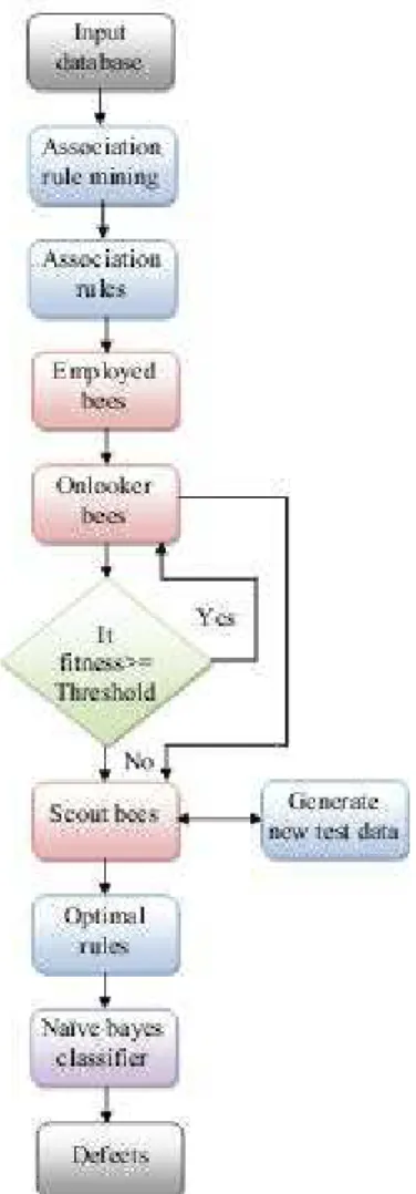
In our previous work, the defect classification was done by association rule mining and decision tree algorithm. Association rule mining algorithm sometimes leads to insignificant rules. So it is very difficult to classify the defects based on these insignificant rules. In order to avoid such issues, we have to optimize the rules before classification based on support and confidence value. In this research, we have focused on finding the optimal rules based on Artificial Bee colony (ABC) optimization algorithm. This will find the optimal support and confidence value to get optimal rules. After getting optimal rules, we will classify the defects based on the naïve bayes classifier. Finally the quality will be assured by using various quality metrics such as defect density, Sensitivity etc. The proposed system will be implemented in JAVA with various data bases in PROMISE data set repository.
3.1. Rule Extraction Using Association Rule Mining
For learning association rules, apriori is a typical algorithm. Apriori algorithm is planned to function on databases having transactions. The apriori Algorithm is a dominant algorithm for mining regular item sets for Boolean association rules. Agrawal and Srikant improved it on 1994. To find association rules on great scale is an innovative way, permitting implication outcomes that contain more than one item. In association rule mining the input given is the database. Two main steps are there in association rule mining. First, using the minimum support value assigned, the frequent item sets are produced. Second, the association rules are produced by means of the frequency item sets produced and the minimum hope value allocated.
To the association rule mining process, a database is given as input. From the input database the number of transactions is computed. For eliminating association rules minimum values of support and assurance should be allocated. The item sets are removed from the database. Every item is the element of set of candidate. The support values are computed for the item sets individually. Using the formula, the support value is worked out
A B
P B A
Support( )
(1)
Where A and B = Frequent item sets.
With the minimum support value, the support values computed for the separate item sets are compared. The item sets with support value less than the minimum support value is removed. The left over item sets are chosen. Next the chosen item sets were united with the same item sets. Based on the support value, once more the support value is computed for the item sets and they are removed. By the eradication and the pruning step the item set which is for producing association rules are found out. By using the formula, the confidence value can be found out
A PB A P B A
Confidence( )
(2) Where A and B = Frequent item sets.
3.1.1. Pseudo Code for Association rule Mining
Ck: Candidate item set of size k Lk : frequent item set of size k Lk = {frequent items};
for (k = 1; Lk !=; k++) do begin Ck+1 = candidates generated from Lk; for each transaction t in database do
increment the count of all candidates in Ck+1
that are contained in t
Lk+1 = candidates in Ck+1 with min_support end
return Ck Lk;
The association rules produced is given as input to the ABC algorithm for optimization. 3.2. Rule Optimization Using ABC Algorithm
Dervis Karaboga explained ABC, is an algorithm in 2005, motivated by the smart behavior of honey bees. The colony of artificial bees has three set of bees in ABC algorithm and they are employed bees, onlookers and scouts. A bee which is remaining on the dance area for composing a selection to accept a association rule is called onlooker and a bee which goes to the association rules that is chosen by the onlooker is called employed bee. The further kind of bee is scout bee that carries out disorderly search for discovering new sources. The place of the association rules represents a realistic solution to the optimization issue and the value of a association rules associated to the quality (fitness) of the associated solution, estimated by,
i i r FIT
1 1
(3) Where
i = number of association rules r = association rules
The main steps of ABC algorithm are: Initialize Association rules
repeat
Place the employed bees on the association rules
Place the onlooker bees on the association rules depending on their nectar amounts Send the scouts to the search area for discovering new association rules
Memorize the best association rule found so far until requirements are met
The collective intelligence of honey bee swarms contains three components. They are Employed bees, Onlooker bees and Scout bees. There are two main behaviors.
(a) Association rules
To choose the association rules forager bee assesses different properties. For effortlessness one quality can be regarded.
(b) Employed bees
The employed bee is used on a particular association rule. It distributes the information about the particular association rules with other bees in the hive. The data which is carried by the bee contains direction, Profitability and the distance.
(c) Unemployed bees
The unemployed bees contain both onlooker bees and the scout bees. The onlooker bee looks for the association rules with the data given by the employed bees. The scout bee looks for the association rules arbitrarily from the environment.
waiting in the dance area. The onlooker bees take the data about the Association rules. Then the employed bees take a trip to their relevant Association rules which they have previously visited and find the neighboring Association rules in comparison via visual information.
At the second step of the cycle, depending on the data given by the employed bees the onlooker bee chooses the Association rules. If the optimization increases the possibility of the association rules selected moreover increases. When the onlooker bee enters in the region as per the data given by the employed bee it selects the neighboring association rules by comparing the values by visual information similar as in employed bees. By the bees on comparison of values based on the visual information, the novel association rules were established. At the third step when the association rules was used by the bees’ novel association rules was found out by the bees. A scout bee arbitrarily chooses the novel association rules and substitutes the old association rules with the novel one. The bee which has the fitness values as excellent sufficient is the result of this fitness. The thorough account of the ABC algorithm is as follows:
Initialize the association rules of the solutionssi,j.
Calculate the population.
Setcycle1; the cycle denotes an iterative value.
Create a solution ui,jin the neighborhood of
s
i, using the following formula: jui,jsi,ji,j
si,jsk,j
(4) Where,k Solution of i
Random number of range [-1,1]. 3.2.1. Pseudo-code for ABC AlgorithmRequire: Max_Cycles, Colony Size and Limit Initialize the Association rules
Evaluate the Association rules Cycle=1
while cy݈ܿ݁≤ܯax_cy݈ܿ݁ݏ do
Produce new solutions using employed bees
Evaluate the new solutions and apply greedy selection process Calculate the probability values using fitness values
Produce new solutions using onlooker bees
Evaluate the new solutions and apply greedy selection process Produce new solutions for onlooker bees
Apply Greedy selection process for onlooker bees
Determine abandoned solutions and generate new solutions in the scout bee section Memorize the best solution found so far
Cycle = Cycle + 1 end while
return best solution
Apply the greedy selection process amid ui,jand si,jbased on the fitness.
Calculate the probability values Pifor the solutions si,jusing their fitness values based on the following formula:
SN i i i i FIT FIT P 1 (5) In order to estimate the fitness values of the solution we have used the following formula:Fig. 1. Architecture of the proposed methodology
Create the novel solutions ui,jfor the onlookers from the solutions sidepending on Piand calculate
them.
Apply the greedy selection procedure for the onlookers amid siand uibased on fitness.
Determine the abandoned solution (source), if exist, replace it with a novel unsystematically produced solution sifor the scout using the following equation:
si,j minjrand
0,1
maxjminj
(7) Memorize the optimum association rules position (solution) attained so far. Cycle=cycle+1
Until, cycle=maximum cycle number.
The ABC algorithm has numerous dimensional search spaces in which there are Employed bees and Onlookers bees. Both bees were classified by their experience in recognizing the association rules. The first population is selected from the employed bee phase. The rules are infatuated by the employed bee. The solution of the employed bee is changed in the onlooker bee stage based on the subsequent formula:
ui,jsi,ji,j
si,jsk,j
(8) Where,j i
s, Solution obtained from the employed bee phase
j i,
Randomly produced number of range [-1, 1]
j
To attain the fitness value, a solution is generated based on the formula and the solution is used in the fitness function. This procedure would last till the whole employed bee gets practiced. The scout bee phase is the ultimate stage of the ABC algorithm. Thus the optimal rules were generated.
3.3. Defect Classification Using Naïve Bayes Classifier
Naïve Bayes algorithm is used to classify the defects. Here the optimal rules were given as input to the naïve bayes classifier. This type of classifier has the advantage that it is easy to implement quickly and generate good results. The Naive Bayes classifier is a probability classifier, based on Bayes’ theorem. Bayes' theorem specifies mathematically the relation between probability of two events A and B.
The Bayes formula is as follows
B P
A P A B P B A P
(9)
Where
P(A) and P(B) are the probability of two events A and B.
P(A|B) is the conditional probability of event A conditioned by event B. P(B|A) is the conditional probability of event B conditioned by event A.
This theorem enables us to determine a conditional probability for the probability of contrary event and the independent probabilities of the events. Thus, we can estimate the probability of an event based on the examples of its occurrence. Here the process is done by the collection of optimal rules. The process is naive Bayesian shows the calculation of probability of occurrence of an event. It is the product of probability of occurrence of defect in the optimal rules. Thus the defects were classified using the naïve bayes classifier. 4. Results and Discussion
The proposed Defect classification system with Naïve bayes classifier is implemented in the working platform of NETBEANS version 7.2 (jdk 1.7) with machine configuration as follows
Processor: Intel core i7 OS: 3.20 GHz
CPU speed: Windows 7 RAM: 4GB
Here we have used some data in PROMISE dataset such as KC1/ software defect prediction. PROMISE refers to Predictor Models in Software Engineering. PROMISE data sets is to handle noise (e.g. with outlier removal, or feature subset selection, or statistical methods that cope with outliers better) or to complete missing data with surrogates from other attributes.
Table 1. Sample rules for defect classification
Coupling between objects
Response for a class
Weighted method
per class Defect
High Medium High True
High Medium Low False
Medium Medium High True
High Low Low True Low Low Low False
4.1. Evaluation of Results
The quality of the system is evaluated using the quality metrics. The quality metrics calculated in our proposed methodology are:
Defect Density Sensitivity Specificity Accuracy 1. Defect density
Defect density is defined as the ratio of total number of defects to the lines of code.
code of Lines
defects of number Total
density
Defect
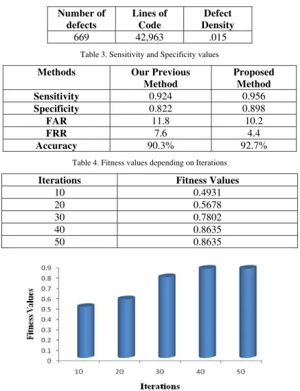
Table 2. Defect Density values
Number of defects
Lines of Code
Defect Density
669 42,963 .015
Table 3. Sensitivity and Specificity values
Methods Our Previous
Method
Proposed Method
Sensitivity 0.924 0.956
Specificity 0.822 0.898
FAR 11.8 10.2
FRR 7.6 4.4
Accuracy 90.3% 92.7%
Table 4. Fitness values depending on Iterations
Iterations Fitness Values
10 0.4931 20 0.5678 30 0.7802 40 0.8635 50 0.8635
Fig. 2. Graph for fitness values based on iterations
2. Sensitivity
Sensitivity (also called the true positive rate) measures the proportion of actual positives which are correctly identified.
fn tp
tp y Sensitivit
(11)
3. Specificity
Specificity measures the proportion of negatives which are correctly identified.
fp tn
tn y Specificit
(12)
Fig. 4. Graph for the comparison of specificity values
4. Accuracy
Accuracy is calculated by considering both sensitivity and specificity factors.
/2
100 FAR FRR
Accuracy (13)
Fig. 5. Graph for the comparison of Accuracy values
From table 3 it is clear that the accuracy of our proposed method performance was higher when compared to our previous methods. Thus the performance measures calculation showed that our proposed method is efficient than our previous method.
5. Conclusion
In our previous work, the defect classification was done by association rule mining and decision tree algorithm. Association rule mining algorithm sometimes leads to insignificant rules. So it is very difficult for defect classification based on these insignificant rules. In order to avoid such issues, we have optimized the rules before classification based on support and confidence value. In this paper we have classified the defects using naïve bayes classifier. The rules were extracted from the input using association rule mining. The rules were optimized using artificial bee colony algorithm. Defects were classified using naïve bayes classifier. The quality was assured using the quality metrics such as defect density and accuracy etc. Our proposed method has achieved an accuracy value of 92.7% which is higher than the existing methods. Thus the performance measures calculation showed that our proposed method is efficiently classify the defects.
References
[1] StefenBiffl and michaelhalling, “Investigating the defect detection effectiveness and cost benefit of nominal inspection teams”, IEEE transactions on software engineering, Vol.29,No.5, pp. 385-397, 2003.
[2] Steven H Lett, “Using peer review data to manage software defects”, IT metrics and productivity, No.2,pp.1-7, 2007.
[3] Suma and Gopalakrishnan Nair T.R, “Enhanced approaches in defect detection and prevention strategies in small and medium scale industries”, In Proc. of the third International Conference on Software Engineering Advances (ICSEA '08), Sliema, pp.389 - 393, Oct. 2008.
[5] Caper Jones, “Measuring defect potentials and defect removal efficiency”, CROSSTALK The Journal of Defense Software Engineering, pp. 11-13, 2008.
[6] Liguo Yu, Robert P. Batzinger, and SriniRamaswamy, "A Comparison of the Efficiencies of Code Inspections in Software Development and Maintenance," In Proc. of International Conference on Software Engineering Research and Practice, Las Vegas, pp.460-465, 2006.
[7] Elish, Karim O., and Mahmoud O. Elish, "Predicting defect-prone software modules using support vector machines", Journal of Systems and Software, Vol. 81, No. 5, pp. 649-660, 2008.
[8] Bibi, S., G. Tsoumakas, I. Stamelos, and I. Vlahavas, "Regression via Classification applied on software defect estimation", Expert Systems with Applications, Vol. 34, No. 3, pp. 2091-2101, 2008.
[9] Chen, Li-Wei, and Sun-Jen Huang, "Accuracy and efficiency comparisons of single-and multi-cycled software classification models", Information and Software Technology, Vol. 51, No. 1, pp. 173-181, 2009.
[10] Chiu, Nan-Hsing, "Combining techniques for software quality classification: An integrated decision network approach", Expert Systems with Applications, Vol. 38, No. 4, pp. 4618-4625, 2011.
[11] Wang, X., Yang, J., Teng, X., Xia, W., & Jensen, R, “Feature selection based on rough sets and particle swarm optimization”, Pattern Recognition Letters, Vol.28, No.4, pp. 459–471, 2007.
[12] Chang, Ching-Pao,Chih-Ping Chu, and Yu-Fang Yeh, "Integrating in-process software defect prediction with association mining to discover defect pattern", Information and Software Technology, Vol. 51, No. 2, pp. 375-384, 2009.
[13] T. Menzies, A. Dekhtyar, J. Distefano, J. Greenwald, “Problems with precision: a response to comments on Data Mining Static Code Attributes to Learn Defect Predictors”, IEEE Transactions on Software Engineering,Vol.33, No.9, pp. 2-13, 2007.
[14] Ouni, Ali, MarouaneKessentini, HouariSahraoui, and MounirBoukadoum. "Maintainability defects detection and correction: a multi-objective approach." Automated Software Engineering, Vol. 20, No. 1, pp. 47-79, 2013.