Time-series properties and empirical evidence of growth and infraestructure: revised version

Time-Series Properties and Empirical Evidence of

Growth and Infrastructure*

I

'li

João Victor

ｾ･ｲ＠

and Pedro Cavalcanti Ferreira

Graduate School of Economics - EPGE

Getulio Vargas Foundation

P. de Botafogo 190 s. 1125-8

Rio de Janeiro,

RJ

2253-900

Brazil

E-mail: jissler@fgv.brandferreira@fgv.br

Revised: September, 1998

Abstract

and Granger-causality tests to examine temporal preoedence of TFP with

respect to infrastructure expenditures. The empirical evidence ia robust in confirmjng the existence of a unity long-run capital elasticity. The analysis of TFP reveals that it is not weakly exogenous in the exogenous growth

modelo Granger-causality test results show unequivocally that there ia no evidence that TFP for both modela precede infrastructure expenditures not

being preceded by it. On the contrary, we finei some evidence that infra&.. tructure investment precedes TFP. Our estimated impact of infrastructure on TFP lay rougbly in the interval (0.19, 0.27).

1. Introduction

After more than forty years studying growth, there are two sty1ized elasses of growth models that have emerged. The first ia that of exogenous growth models,

based on Solow(1957), Cass(1965) and Koopmans(1965), and the second is that of

endogenous growth models based on Romer{1986, 1987, 1989), among others. The first basic difference among these two classes is the behavior of productivity. For the exogenous elass, productivity is assumed to grow at an exogenous rate. This implies a balanced-growth path for macroeconomic aggregates, and thus a unity long-run capital elasticity in production. Because models in this tradition use the condition of decreasing returns to capital for the existence of equilibrium, the only way to assure growth in steady-state is to require exogenous technological change. In the endogenous class of modem this condition is dropped since it is thought to be too ad hoc. To assure growth, extemal efIects due to social capital are introduced, although decreasing returns to private capital are still maintained. The extemality hypothesis by itself does not guarantee growth, since it is still possible that the marginal product of capital (private plus social) will converge to

zero. For example, with Cobb-Douglas technology, unless the long-run elasticity of capital is at least one there wiIl be no growth in steady-state. Df course, if the long-run elasticity is above unity there wiIl be explosive growth. Since this is not a stylized fact of modem economies, testing the extemality hypothesis has focused on the case of unity elasticity. A consequence of a unity elasticity is that macroeconomic aggregates wiIl foIlowa balanced-growth path. Regarding productivity, little or nothing is imposed in the class of endogenous growth modem. From the discussion above, it is clear that these two models are observationally equivalent regarding (i) a balanced-growth path for macroeconomic aggregates,

and specifically (ii) a unity long-run capital elasticitYj see Lau and Sin(1997a). Thus, estimating long-run elasticities cannot be a strategy in distinguishing which of these models best fit the data. Despite that, short-run capital elasticities differ for both models. For the endogenous class it is also one, but for the exogenous class it wi1l usually be lese than unity, reftecting the fact that there are decreasing marginal returns in equilibrium.

Since the observational equivalence result is relatively new, before it became

known several authors have tried to confirm the theoretical predictions of a given model class by examining long-run elasticitiesj see Neusser(1991), who finds support for the exogenous-growth model using cointegration, and the cross-country study in Romer(1987) , who finds a unity capital elasticity supporting the endogenous-growth model. Another problem of econometric testing of growth models is that not alI studies were careful in distinguishing between the short-and the long-run capital elasticity. For example, the ｴｩｭｾｳ･ｲｩ･ｳ＠ evidence in

Romer(1987) and Benhabib and Jovanovic(1991) inter-alia reject a unity capital elasticity. The data used in these regressions are either first- or quasi-differenced, which raises the issue of what coefficient is being estimated. One the one hand, if there is no cointegration in the data, one can estimate consistent1y the short-run capital elasticity from first-differenced regressions. Regarding quasi-differenced regressions, consistency will depend on common factors being correctly imposedj see Hendry and Mizon(1978). On the other hand, if there are long-run relation-ships, ignoring them yields inconsistent estimates of short-run elasticities in both

cases.

There are several aspects of growth models that have to be taken into account for successfully assessing their fito These issues have not been thoroughly dis-cussed by the literature. Moreover, they have not been used appropriately when confronting theoretical models with the data. In this paper, we first set out what are the main ｴｩｭｾｳ･ｲｩ･ｳ＠ properties of growth models regarding: the order of ｩｮｾ＠

gration of macroeconomic aggregates, the cointegration relationships implied by

model is (weakly) ex:ogenous. For the endogenous growth model, we investigate the properties of a new Solow residual, taking into account a unity long-run cap-ital elasticity. Finally, for the Solow residuals of both models, we estimate what is the long-run impact of infrastructure ex:penditures following Aschauer.

To estimate and test long-run elasticities we use cointegration techniques as proposed by Johansen(1988, 1991), where estimation and testing are alllikelihood-based. TFP exogeneity testa are based on the typology of Engle, Hendry and Richard(1983), and performed according to Johansen(1995, pp. 122-123). Granger-causality tests for TFP and infrastructure investment take the form of ex:clusion testa, where we take into account the criticism of Toda and Phillips(I993) of such

testa.

Section 2 presents a discussion of a stylized version of both theoretical models, showing the observational equivalence resulto It also diSCU88eB the properties of TFP for both models. Section 3 presents a discussion of the recent applied liter-ature using our previous theoretical results. Section 4 presents the econometria techniques used on the empirical section. Our empirical results are presented in Section 5, and Section 6 concludes.

2. Theory

2.1. Stylized Growth Models

This section diSCU88eB two distinct classes of economic models: endogenous and exogenous growth models. We present here stylized versions of these models under very restrictive parameterizations of preferences and technology, wbich capture the essence of the long-run co-movement in the data we want to discuss. Although these stylized facts could be discussed under a less restrictive setting, we chose their restricted version for expositional reasons.

Under Cobb-Douglas technology, Romer's(1986, 1987, 1989) endogenous growth mo deI can be characterized using a representative consumer who maximizes bis/her flow of utility, choosing a sequence of consumption {Gt } subject to a resource

con-straint:

00

B.t.

Gt+lt

-

Y, = A

Kf

LP-o)

Jr,

ex}> (Zt)

Kt+l

-

It

+

(1 - 6) Kt

O

_<

{3

<

1, (2.1)

where

Yt

is output, Kt is the stock of capital,

Lt

is hours worked, Ic is investment, 6 is the depreciation rate of the capital stock, Ec (.) is the conditional expectation operator, and {Zt} is the stochastic process representing productivity. Aggregate capital per capita (Kt) is included to represent the extemalities due to the fact that knowledge is non-appropriable.

In equilibrium we have Kc = n. (Kt/

Lt),

where n is the number of firmsl. In

per-worker terms the production function is given by

(Yt/

Lc)

=

A (Kc/

Lct

[no

(Kt/

Lc»)'

exp (Zt). Hence, the (private) marginal productivity of capital is given by:

After solving the representative consumer's problem2 _{the growth rate of the} economy (-y) is given by:

1

+

'Yc - Ec

[F

K / L (.)

+

(1 - 6)] {3

- Ed

Q A n' (Kt! L_t)(0+9-1) exp (Zt)

+

(1 - 6)] {3. (2.2) If Q

+

(J

<

1 the model displays no growth. H Q

+

(J = 1 the mo deI displays

sustainable growth as long as Q A n' Et [exp (Zt)]

+

(1 - 6) is greater than 1/{3. If

Q

+

(J exceeds unity there will be explosive growth, which is not a stylized fact of

modem economies. Under this conjecture, testing this class of endogenous growth models amounts to checking if Q

+

(J = 1. Under this condition, the growth rate

of the economy is stationary, although (log) ｯｵｾｰｵｴ＠ itself will be a non-stationary process growing at rate 'Y.

Exogenous growth models inspired in Solow(1957), Cass(1965) and Koop-mans(1965), and upclated by King, Plosser and Rebelo(1988) and King, Plosser,

1 Romer(1989) assumes that the number of firms and consumers is the &ame, 80 that K,/ L,

stands both for capital per labor and capital per firmo

2Note that equilibrium is guaranteed because the technology still displays coostant returns-to-eca1e to private factors and because the whole sequence {1<,}:O is taken as given when the CODSumer solves his/her problem. Only then is the equilibrium condition K, = n . (KeI L,)

Stock, and Watson(1991), will display growth of output per-capita as long as

productivity grows exogenously. Otherwise, decreasing marginal returns will

ul-timately imply no input growth, and thus, under appropriate conditions, per-capita output will reach a steady-state value. Using Cobb-Douglas technology and a random walk productivity process growing at rate p on average, In (Wt) =

p

+

In (Wt-l)

+

Ef,

the problem faced by the consumer is the following:

00

Max

Eo

L

ptu

(C,),

{cc} t=O B.t.

C,+lt

-

Yi =

A

ｋｾ＠ QI-0)Wt Kt+l

-

1t

+

(1- 6) Kt

O < (3<1

O < a<l. _(2.3)

After solving the consumer's problem the growth rate of the economy (p) is given by:

1

+

JJt - Et [FK/ L (-)

+

(1 - 6)] {3

- Et [a A (Kt/ Lt)(O-l) Wt

+

(1 - 6)] (3. (2.4)

We now discuss some revealing time-series properties of these two classes of growth models.

Proposition 1. In the problem (2.1), under a

+ ()

= 1, log-utility, and

fulJ-depreciation of the capital stoclc, the closed-form solution for In (Kt+l) implies it has a unit root even with {Zt} stationary. Since the closed-form solutions for

In (yt), In (C,) and In (lt ) are linear functions of In (K_{t ),} they all have common

unit roots. Hence, they cointegrate in such a way, that,

In (yt) - In (Kt ), In (lt ) - In (yt) , and,

In (C,) - In (Yi), _(2.5)

form a basis for the oointegrating sp&ee. This is true, regardless of the persistency

i.i.d. process,

stationary

ARM A(p, q) process,

or

stationary ARM A(p, q)

process about a time trend.

Proof. Wben solving this problem, the consumer takes the sequence

{Kt}::

parametrically. Tbus, the problem reduces to a standard log Cobb-Douglas

dy-namic optimization. Under tbese assumptions, it is a well known result (Sargent, 1987, chapter 1) that there ia a closed fonn solution to this problem, it being straightforward to sbow that:

(2.6)

In equilibrium,

Kc

= n .

Kcl Lc.

Thus, tbe law of motion of the log of capital per bour can be written as:

(2.7)

Wbere 1-'1 includes fixed parameters from preferences and technology. When Q

+

8 = 1, capital per bour bas a unit root and (lagged) equation (2.7) is:

In (Kt! Lt) = 1-'1

+

In (Kt-l1 Lt-1)

+

Zt-l·

Using this resu1t in tbe decision roles and output equation we obtain:

In (Ytl Lt) - 1-'2

+

In (Kt! Lt)

+

Zt,

In {C ti Lt) - 1-'3

+

In (Ktl Lt)

+

Zt,

In (ltl Lt) - 1-'1

+

In (Ktl Lt)

+

Zt,

(2.8)

(2.9)

Since In (Kt!Lt) is 1(1), and output per hour, consumption per bour and invest-ment per bour contain In (Kt! Lt), they are all 1(1) as well. Cointegration as postulated in Proposition 1 above follows immediately from subtracting respec-tively In (Ktl Lt) from In (Ytl Lt), In (Ctl Lt) from In (Ytl Lt),and In (lt! Lt) from In (Ytl Lt), using tbeir expressions in (2.9) .•

Proposition 1 ofIers an empirical test for the necessary condition of the in-creasing retums bypothesis3 • H Q

+

8 = 1, the variables in the model will have

unit roots. Moreover, they will cointegrate with known coefficients given by (2.5)

above. For example, there is a unity long run elasticity between In (Y,J

Le)

and

In (K,/

Le),

or between In (Yí) and In (K,). .

Although unit roots and restrictions (2.5) on cointegration coefficients are a necessary condition for the increasing-returns hypothesis, theyare not sufficient for it. Benhabib and Jovanovic(1991) note that when the data have unit roots, it does not necessarily follow that Q

+

O = 1. As discussed by King, Plosser

and Rebelo(1988), and by King et al.(1991), restrictions (2.5) on cointegration coefficients are also present in the standard neoc1assical growth model with a random walk (log) productivity process presenteei above". We thus present a second resulto

Proposition 2. In problem (2.3), under log-utility, full-depreciation ofthe capi-tal stock, and a random-walk (log) productivity process, In (Wt) = p+In (Wt-l)+4',

the closed-form solutions for In (Yí) , In (Ct), In (K,) and In (/t)5 are linear func-tions of the same forcing variable (In (Wt)). Hence, these variables &bare a common

unit root, and cointegrate in such a way, that,

In (l't) -In (Kt ), In (/t) - In (Yt) , and,

In (Ct ) -In (Yí) ,

form a basis for the cointegrating space.

Proof. See King, Plosser and Rebelo(1988) and King et al.(1991) .•

In Proposition 2 the variables of interest still cointegrate with the same coef-ficients of (2.5) despite the fact that O

<

Q

<

I, Le., despi te decreasing returns to

scale. Comparing this result to that of the endogenous growth model illustrates a major difference: for the latter, growth, integration, and cointegration follows be-cause agents do not consider their external eft'ect when buying an additional unit of capital. When the externaI effect has the "right impact on output," Le., O = 1- o, this extra unit of capital is just enough to make the aggregate capital stock (Kt)

grow in equilibrium. This leads to identical steady-state growth for alI variables of interest, i.e., cointegration. For the exogenous growth model, cointegration is obtained forcefully tJia the productivity process, since it is a consequence of the

"This l'E'Bults generalizes for any 1 (1) productivity proal88.

existence of this unique integrated forcing variable

(In

(Wt», which dominates all the long-run co-movement properties of the aggregates in the system.

Despite these conceptual dift'erences, Propositions 1 and 2 show that endoge-nous and exogeendoge-nous growth modela are observationally equivalent with respeet to cointegration restrictions. This was prove<! by Lau and Sin(I997a), although the initial idea can be traeed back at least to Benhabib and Jovanovic(I991)6.

2.2. Solow Residuais of Growth Models

Despite the fact that the endogenous and exogenous growth modela are observa-tionallyequivalent with respect to cointegration restrictions, their Total Factor Productivity (TFP) processes have quite dift'erent properties. The first dift'erence is about their order of integration.

Proposition 3. Given the assumptions in Propositions 1 and 2, if

In

(Yt/4.) ,

In (Ct/4.), In (Kt! 4.) and In (lt/4.) are a11 integrated processes of order one (I (1», then the TFP proce9;es ofthe endogenous growth model is I (O) whereas

the TFP process of the exogenous growth model is I (1). More genera11y, jf

In (Yí/4.), In (Ct!

4.),

In (Kt/4.) and In (lei 4.) are al1 integrated processes of

order d (I (d», it fonows that the TFP process of the endogenous growth mode1 is I (d - 1) whereas the TFP proce9; ofthe exogenous growth model is I (d).

Proof. From equation (2.7), under Q

+ ()

=

1, it follows that:

(2.10)

which establishes that the TFP process of the endogenous growth model is I (O).

Notice that the only way to have Zt being 1(1) is having !:lIn (Kt+l/ Lt+i) being

I (1) as well. But this makes

In

(Kt+l/ Lt+l) and all other variables of interest

I (2) processes. For the exogenous growth model, the order of integration of In (Yí/4.) , In (Ct!

4.),

In (Kt/4.) and In (lt/4.) must be the same ofthat ofIn (Wt).

Then it follows that In (Wt) is 1(1). Generalizing the proof for the I (d) case is straightforward. From (2.10) it is obvious that In (Kt+t! Lt+l) (and all other variables of interest) is of one order of integration higher than Zt, and thus the

result follows .•

Another key difl'erence about TFP processes is the exogeneity assumption on the process:

In

(Wt)

= P.

+

In

(W,-l)

+

Ef·

Since the growth rate of productivity is given by:

AIn{w,)

=p.+Ef,

it will grow exogenously as long as there are no external factors inftuencing

{Ef}.

On the class of endogenous growth models little is imposed on

{Zt}.

In particular, the exogeneity assumption used on the other class of growth models is either dropped or omitted. Hence, we refrain from testing its exogeneity status.

Measuring TFP for the endogenous-growth model is straigthforward once a consistent estimate of 0+9 is obtained. Labelling

ri:

its Total Factor Productivity, and recalling that in equilibrium

Yt/

Lt

= A exp (ZtJ (Kt/ Ltt (n . K,/

Lt)',

we

have, after a logarithm transformation, and under 0+9 = 1:

ｰｾ＠ = (y, -4) - (k, - lt) = y, -

kt

=

a+z,

(2.11)

where lower-case characters denote logarithms, and

a

= In

(A

n').

TFP is equal to the Solow residual (Zt) (up to a constant). Thus, TFP, or the (demeaned) Solow residual, can be easily calculated using y, - k,.

For the class of exogenous-growth models, calculating its TFP requires a con-sistent estimate of o. Labelling

11':

as its TFP, we obtain after similar manipula-tions:

li:

= (y,

-4) -

o(k,

-4)

=

ln(A)+ln(w,). (2.12)

Once again, TFP, or the (derneaned) Solow residual, can be easily calculated using

(y, - I,) - o (k, - I,).

2.3. Infrastructure Expenditures, Growth, and Solow Residuais

output not captured by input variation. In a typica1 paper, researchers investigate whether the behavior of "Solow residuais" could be explained by the behavior of a set of economic variables. A vintage of this literature has focused on the role of infrastructure. Aschauer(1989), Nadiri and Manuneas(1992) and Munnell(1990),

suggested that the behavior of the Solow residual, and thus productivity, can be partial1y explained by the evolution of public infrastructure. For example, public infrastructure investment per hour (G,/ Lt) could be a separate argument of the production function. In this case, TFP could be decomposed into two parta, a non-modelled one, and a modelled one - capturing the efl'ect of (Gt/L,).

An alternative way of modelling the infra&tructure efl'ect is to inc1ude infras-tructure capital as an input of the economy's production function. This has been tried by Lau and Sin(1997b), but the approach has been criticized by Bougheas and Demetriades(1997) for lacking a fundamental explanation of the infrastruc-ture role in production. Bougheas and Demetriades, on the other hand, propose

"introducing infrastructure as a technology which reduces the fixed cost of pro-ducing intermediate goods," Le., specialization. A by-product of it is a non-linear relationship between infrastructure capital and growth.

Regardless of how the role of infrastructure is modelled it is interesting to inves-tigate the following issues for the two classes of growth models considered above:

Is TFP of the exogenous growth model (weakly) exogenous when we consider

infrastructure expenditures? For the two models considered, do movements in in-frastructure precede or are preceded by movements in TFP (Granger-causality)? For the two models considered, what are the long-run elasticities of TFP with respect to Infrastructure? Is there a non-linear relationship between TFP and infrastructure expenditures for the two models considered here (Bougheas and Demetriades )?

3. Previous Empirical Results

recently the obeervational equivalence of these models became a well known fact (Lau and Sin(l997a», there have been several studies in the past that used long-run capital elasticities to

confirm

or dismiss the fit of the sty1ized versions of the

exogenous or the endogenous growth model presented above; see Neusser(1991),

Romer(1987), and Ferreira(1993).

The evidence that the long-run capital elasticity ia unity is abundant:

1. Cross-country studies: using data from Maddison(1983) on cross-country rates of growth, Romer's(1987) physical capital estimate is 0.87 and not significantly difIerent from one. With the Summers and Heston(1991) data base, bis estimated coefficient is 0.75. Ferreira's(1993) cross-country studies reach a similar conclusion using data from Summers and Heston(1991), the IMF, and Benhabib and Spiegel(1994). Physical capital coefficient estimates are usually close to one and very robust to changes in the specification of the model or to changes of the data used.

2. Time-series evidence: using data in leveis and cointegration techniques, Neusser(1991) confirma the theoreticallong-run elasticities in either Propo-sitions 1 and 2 above. Benhabib and Jovanovic(1991) running a regression in leveis with annual data, find a capital-elasticity estimate of 1.06; see Ta-ble 7, p. 91. Using data from Maddison(1983) on three G-7 countries, Lau and Sin(1997a) find evidence supporting cointegration between output and capital, although the capital elasticity is far from unity in some cases.

Despite this favorable evidence some time-series studies have found a capital elasticity estimate far from unity. In Romer's(1987) article, when annual or decade data in first differences are used, results show a large and significant coefficient for the labor input and an insignificant coefficient for the capital input. The same pattern is found by Benhabib and Jovanovic, who applied maximum likelihood to U.S. data with the error term assumed to be an ARMA (1, 2) processo For quarterly data, they find a labor coefficient of about 0.65 and estimated ct

+

8

case, even if there are no long-run relationships in the data, inconsistencies will

arise due to imposing common factors.

The relationship between public infrastructure and productivity was discussed and tested originally by Aschauer(1989). Using time series data, Aschauer's es-timate of the efJect of public capital on

TFP

is about 0.50, which is relatively

high. Munnell(l990) using regional data concurs with Aschauer's estimates.

Cost

function duality estimates at the industry leveI by Nadiri and Manuneas(1992) and Morrison and Schwartz(1992) are relativeIy smaller (roughly 0.15) but

con-firm Aschauer's initial premise. The same applies to the cross-country evidence in Ferreira(1993) and Easterly and Rebelo(1993). More recently, Bougheas and Demetriades(1997) estimate a non-linear relationship between infrastructure cap-ital and growth, finding an inverted U-shaped relationship between them.

In most cases, the empirical evidence tends to confirm a supply side role for govemment (or private infrastructure in some cases) affecting productivity.

Ex-ceptions are Hulten and Schwab(1992), using a growth accounting framework, and Holtz-Eakin(1992), using panel data at the state leveI. Although causality between productivity and public infrastructure is crucial for this discussion, it has not been thoroughly studied7•

4. Econometric Tests

As discussed in the previous section, both endogenous and exogenous growth models are observationally equivalent with respect to cointegration tests. There-fore, the initial step in our empirical investigation is to examine whether U.S. aggregate data conform to these theoretical long-run restrictions. In doing so,

we are not testing any of these two models, but a broader class of models that include both. Before cointegration tests are performed, we investigate the order of integration of the data using the Augmented Dickey-Fuller testj see Dickey and Fuller(1979, 1981). There are several cointegration tests in the literature, which is now well known. Gonzalo(1994) compares their properties and concludes that Johansen's(1988, 1991) likelihood-based method is the most adequate overallj see Johansen and Juselius(1990) for an application. The test consists of estimating rthe number of linearly independent cointegrating vectors (or cointegrating rank)

and the corresponding cointegrating vectors by maximum 1ike1ihood. Two statis-tia can be used for estimating r: the 7mce and

.\mu.

statistics, which have non-standard asymptotic distributions. Moreover, the tedmique has the advantage of allowing testing hypotheses on cointegrating vectors, conditioned on knowledge of r. These testa are the usuallikelihood-ratio testa and have the nice property that their limiting distribution is

r.

The relationship between growth and infrastructure will be investigated in

several ways. Regarding Solow residuaIs of exogenous growth models we will perform exogeneity tests using the typology of Engle, Hendry and Richard(1983). Suppose that we are interested in conducting inference on a given set of parameters

{j, and have two series re, and Se. Then, re is said to be wealdy exogenous for {j

I

if we can factor the joint density of (re, se) ,

f

(re, se), into the conditional and marginal distributions, 9 (Se Ire) and h (re) respectively, where the parameters of the joint and of the marginal densities are separable in such a way that, to learn {j,

one does not need to conduct inference on the parameters of the marginal density

h (re). This "separation" property allows doing conditional inference on {j using

rt. Strong exogeneity for (j requires, in addition to weak exogeneity, that rt is not

Granger-caused by St. If this is not the case, it is impossible to do conditional

forecasting for St, since one needs to learn St in order to learn the future of rt.

Weak exogeneity tests will use the results in Johansen(I995, pp. 122-123). There, it is shown that, under cointegration, weak exogeneity can be tested via

the significance of the error-correction tenn(s). Granger non-causality tests will take the usual format of testing for exclusion restrictions. Toda and Phillips(1993) show that these test results can lead to wrong inferences when the number coin-tegrating vectors in the system is unknown. We thus present test results under a variety of assumptions regarding cointegration between Solow residuaIs of the exogenous growth model and infrastructure expenditures.

5. Empirical Results

5.1. The Data Set

The data set used consists of U.S. Post-war quarterly log of private GNP Yt, log of hours worked lt, log of the capital stock

ke,

log of public investment on

total GNJ>8. Houra worked used the Household Survey monthly series cumu-lated to generate quarterly figures. Public investments in infrastructure represent the sum of federal, state, and local non-military expenditures on structure and durables. Capital stock data were constructed using the gross private domestic investment series, accumulated using the perpetuaI inventory method at three dif-ferent annual depreciation rates: 6%, 8% and 10%. The initial capital stock was calculated following Young(1995).

All

these series were extracted from Citibase and are available from 1947:1 through 1994:3 in most cases. The exceptions are

l"

for which data are available from 1947:1 through 1993:4, and O" available from 1959:1 through 1994:3. We a1so used an additional version of the capital stock

series, based on the annuaI figures provided by the Survey of Current Business. These data were interpolated by the FED to yield quarterly observations in order to run the MPS model, and are available from 1958:1 through 1988:4. Figure 1 displays the production function data. Notice that although all series show signs of non-stationarity, Yt - lt and

kt

-l, follow each other very closely in the sample period.

5.2. Unit Root8 and Cointegration

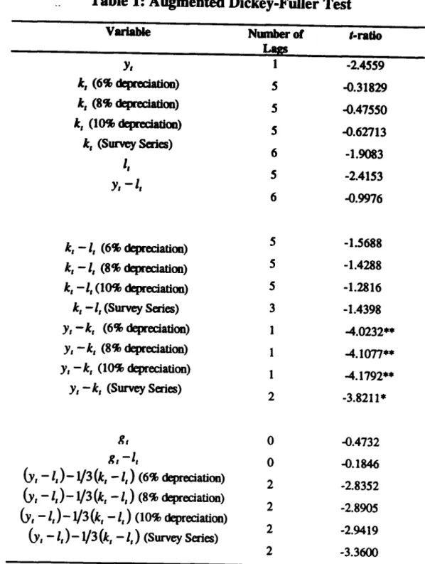
The first step is to test the data for unit roots, since it only makes sense to test for cointegration if they have a long run component. The Augmented Dickey-Fuller test was used including a time trend and a lag structure necessary to obtain white noise residuals°. Results are presented in Table 1. At usual significance leveis, we cannot reject the hypothesis that y" lh k,., Ot, Yt -lt, and Dt -l, contain one unit root. However, for Yt - kt, we do reject the presence of a unit root, regardless of the version of the capital stock series used. This result is promising, since it is an indication that Yt and kt , may be proportional in the long run.

Cointegration tests were performed using two distinct data sets in forming the Vector Autoregression (VAR). The first uses the variables in the aggregate production function in per hour terms, Le., Yt -lt and kt -lt, and the second uses 8This is ao importaot differeoce betweeo Dor data set aod the Doe used by Lau aod Sin(l997a). Using private GNP may be criticaI io investigating a uoity elasticity for the two modeJs consid-ered. With the goveroment sector included, there is the poteotial to depart from uoity capital elasticity, sioce fiscal variables may be used to do systematic couoter-cyclical policies. This is exactly their fioding.

°We started the lag search with 8 lags going dowo by Doe lag up to lag zero. The oumber Df

alI three variables in the production function, i.e.,

Yt, lt

and

ke.

For the bi-variate V AR, the existence of a long run relationship requires

Yt-lt

and kt

-lt,

to cointegrate with the cointegrating vector given by

(1, -1)'.

The first step in applying Johansen's cointegration test is to determine the order of the

VAR, and decide how to model its deterministic components. The lag-order search

was accomplished using the Schwarz criterium in conjunction with diagnostics testslO• The VAR was estimated with a constant, seasonal dummies, and a linear trend term, since the data in leveis, and Yt -

ke,

show signs of containing a linear trend. The VAR order chosen for the diflerent versions of the constructed

ke

-lt,

was three, but five lags is also a possibility. For the Survey of Current Business version of

ke

-lt,

the lag order chosen is three. Cointegration tests were performed using these lag structures. There is overwhelming evidence that there is one cointegration vector. Conditioned on the cointegrating rank being one, we tested

the restriction that the VAR does not contain a time trend. For alI cases this restriction is strongly rejected, supporting the initial guess that the VAR should be modelled with the trend presente

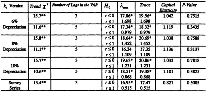
For three lags, the results of cointegration tests reject that there are zero cointegrating vectors for alI versions of the calculated

ke

-

lt as shown in Table 2. Moreover, the hypothesis that there is one cointegrating vector cannot be rejected for alI cases at usual confidence leveis. Estimates of the long run elasticity of capital per hour are alI marginally higher than one. To test if they are equal to one, we used the likelihood ratio test proposed in Johansen(I991), conditioned on the cointegrating rank being one. The Results show that a unity coefficient cannot be rejected in alI cases with very high confidence. For the Survey of Current Business version of kt

-lt,

at three lags, we reject the null of zero cointegrating vectors with 95% confidence using the Àm-statisticll. Moreover, we cannot reject that the cointegrating rank is one using the trace and the Àm- statistic.· Capital per hour long run elasticity is estimated to be 0.82. At usual confidence leveis, conditioned on one cointegrating vector, we cannot reject that it is unity.

For five lags, we found very similar results for kt -

lt.

One cointegrating vector is found for alI but one version of capital per hour (8% depreciation) at 5% significance. However, at 10% significance, there is one cointegrating vector

lOThe first is helpful to decide on the trade-off between degrees of freedom and nsidual sum of squares, but has little information on whether the model p888E8 specification testa.

11 With 90% oonfidence, both the >.m- and the Trace statistic reject that the oointegrating

for all versions of the capital stock. Conditioned on rank one, we cannot reject a unity long run elasticity for kt - lt.

Thus, for the bi-vanate VAR, there is overwhelming evidence that output per hour and capital per hour have a long run relationship with unity elasticity, con-forming to the two models described above. This evidence is robust to variations of the capital series used or to variations in the lag length of the VAR.

We now tum to the evidence of the tri-variate VAR using Yt, lt and

kt.

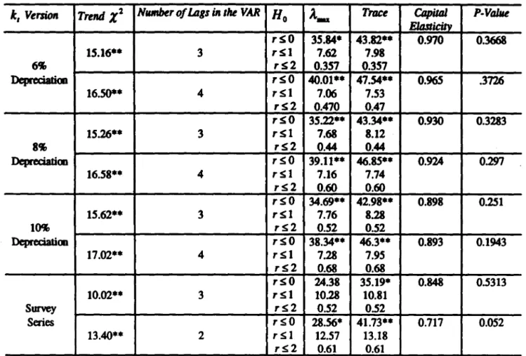
Based

on statistical tests in Table 3, we found again that all VAR's should include a constant term, seasonal dummies, and a time trend termo For the constructed version of

kt

,

the preferred lag order is three, but four lags is a1so a possibility. For the Survey of Current Business version of

kt

,

we choose a VAR of order two, but order three is also possible.

Using the VAR with 3lags, for the constructed kt, we found vast evidence that there is one cointegrating vector. In the long run relationship, point estimates for the capital coefficient are all around 0.9, and those for hours are all near zero. We thus tested the joint hypothesis that the latter is zero and the former is one. For all three versions of kt we could not reject it, Le., Yt - kt is stationary12. These results are robust to changes in the lag order, as can be seen for the results using four lags presented in Table 3.

The analysis for the Survey of Current Business version of

kt

yields slightly different results, in which finding a long run unity elasticity depends on the lag length used. For three lags, conditioned on one cointegrating vector, we cannot reject unityelasticity. However, with two lags, we marginally reject it. The results of the Monte-Carlo exerci se in Gonzalo(1994) suggest preferring the results with a higher lag order, since omitting the dynamics in cointegrating analysis may lead to inconsistent estimates of cointegrating vectors.

Overall, the outcome of unit-root and cointegration tests confirm the adequacy of the two growth models discussed above.

5.3. Is Exogenous-Growth TFP Exogenous?

For the exogenous growth model we impose (}

=

!

in constructing its Solow residual. This estimate is by far the most widely used for that purposej see Cooley and Prescott(1995) and McGrattan(1994). The ADF integration test suggests

that the Solow residual is an integrated process of order one for the exogenous

growth model under Q =

i.

Next, we investigate the exogeneity of TFP by setting

up a V AR including the ex:ogenous-growth Solow residual and (log) infrastructure expenditure per-hour 9t -lt. Plots of bit -I,) -

i

(ke

-4)

and 9,

-4

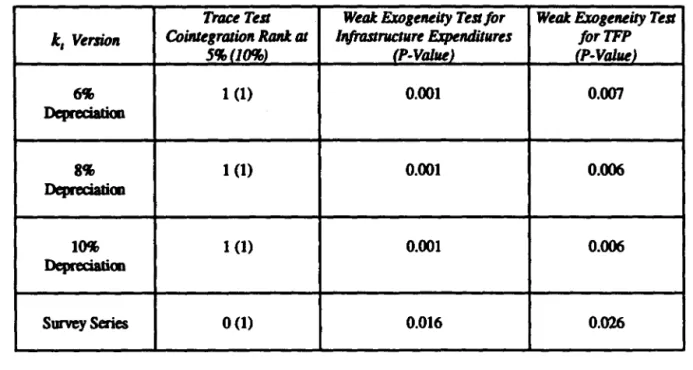
are shown in Figure 2. Exogeneity-test results are presented in Table 4. The lag length chosen is four and all VAR's include a constant, a time trend, and seasonal dummies. Cointegration testa reveal that TFP and infrastructure expenditures have a long-run re1ationship. At 10% significance and using the 1hJce test statistic, there is one cointegrating vector for all versions of the capital stock used. At

5%

there is one cointegrating vector for all capital stock series but the Survey series. Conditioning on the ex:istence of one cointegrating vector, we reject the hypothesis that TFP is weakly ex:ogenous for the parameters of interest in the conditional model using infrastructure expenditures. Note, however, that infrastructure expenditures are not Weakly Exogenous either for the parameters of interest in the conditional model using TFP.

5.4. TFP and Infrastructure in Endogenous and Exogenous Growth Models

In this section, given our previous empirica1 results, it is natural to label (Yt -

ke)

as the Solow residual of the endogenous-growth model. As discussed above, for the exogenous-growth model we use Q =

i

in constructing the Solow residual.

For the endogenous growth model, Granger non-causality test results between TFP and 9t -

4

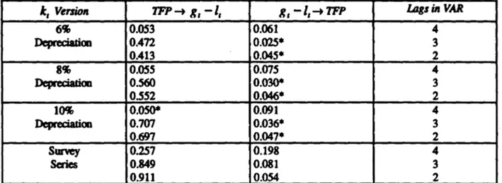
are presented in Table 5; see Figure 3 for plots of the data. Since there is an imbalance between the order of integration of the Solow residual {which is I (O» and 9t - lt {which is I (I», we use the former in levels and the infrastructure expenditures series in first differences. It is well known that causality-test results depend on the lag structure of the VAR. Thus, we present them for lag orders four, three, and two. At the 5% significance leveI, in all cases but one, there is no Granger-causality from TFP to 9t -

lt

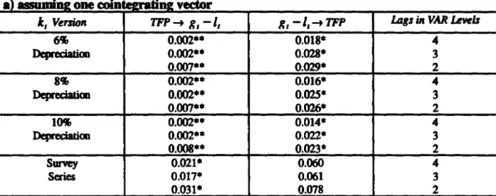
13. On the other hand, we find that 9t - lt Granger-causes TFP for almost every lag structure.

For the ex:ogenous growth model, Granger non-causality test results between TFP and 9t -lt are presented in Table 6. Since both series are I (I), the

distribu-13Notice that with a VAR of order 4, Granger-causality p-values are very close to 0.05, a

tion of the test statistics depend on whether or not the two series are cointegrated; see Toda and Phillips(1993). Thus, we chose to present test results for the case of no cointegration and of one cointegrating vector, ruling out the case where both series are

I

(O).

H

there is one cointegrating vector, test resulta ahow that there ia feedback for all accumulated capital series at 5% aignificance, i.e., Granger causality in both directions. For the Survey series there is weak evidence that

TFP

Granger-causes infrastructure expenditures: no-causality from infrastruc-ture expendiinfrastruc-tures at 5% but causality at 10%. Thus, we conclude that ge -

lt

Granger-causes

TFP

and that the reverse ia also true. H there ia no cointegration test results are very different: there ia no Granger causality in either wayat 5%. At 10% there is weak evidence of causality from 9t -

lt

to TFP.

Putting all these results together, it is clear that we can state unequivocally that there is no evidence that TFP precedes infrastructure expenditure and that it ia not preceded by it. Moreover, there ia some evidence that 9t -

lt

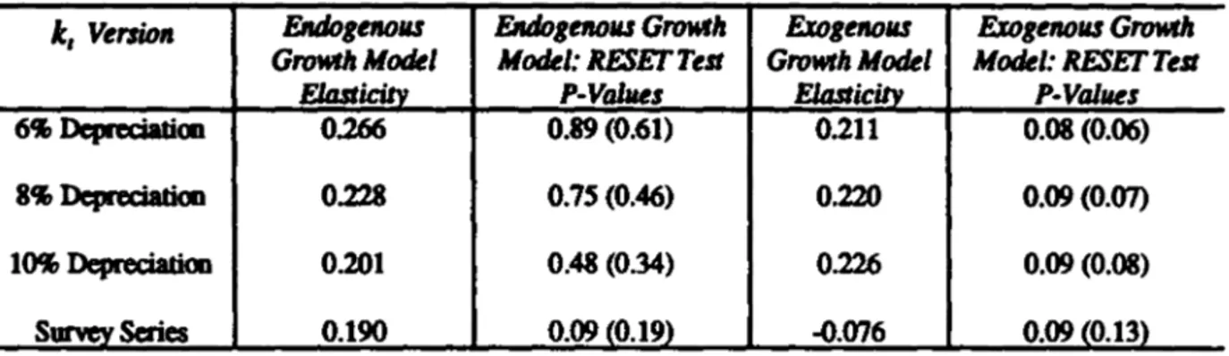
Granger-causes TFP, not being Granger-caused by it. The evidence ia strong for the endogenous growth model, but, for the exogenous growth model, these resulta depend on whether or not the two series are cointegrated. If we take into account cointegration-test results, we find weak evidence that ge - it precedes TFP (10% significance). However, as pointed-out by Toda and Phillips, these test results can be mialeading.

The next atep in our empirical investigation is to calculate the infrastructure elasticity of Solow residuaIs for the two growth models. Results are presented in Table 7. For the endogenous growth model, due to the imbalance in orders of integration between Yt - kt and Dt - it , usual statistical inference is invalid, but consistent estimates can atill be obtained. Elasticities are calculated from the static (long run) solutions of the VAR in leveis using different versions of Yt-kt and

The final atep of our empirical investigation of TFP and infrastructure expen-ditures ia to perform diagnostic tests on the estimated linear models (Table 7). We use the RESET test for non-linearity (Ramsey(I969», including initially a quadratic projection term, and then a quadratic and a cubic term jointly. The results are clear: for the endogenous growth model, there ia almost no sign of misspecification of the estimated linear relationship. The exception being the re-gression run with the Survey series. For the exogenous growth model, using the 10% significance leveI, all models show signa of misspecification, although at the 5% leveI they do noto

For the endogenous growth model, these results confirm the existence of a supply aide role for govemment infrastructure expenditures. It indicates that an increase in public infrastructure affects productivity positively and thus the marginal returns to capital and labor. On average, if there are better roads, porta, communication systems, etc., the same ftow of private capital and labor services

is able to produce the same output faster or a higher output in the same amount

of time. According to our results, a 10% increase in public infrastructure outlays

boosts TFP in the long run by appraximately 2%. Since U.S. public expenditures

in infrastructure decreased in the 1970's, only reverting this downward trend in the mid 1980's, this can partially explain the observed productivity slowdown for this period. Although with different magnitudes, this result agrees with

As-chauer(1989) and Morrison and Schwartz(1992), who used a completely different methodology in investigating the role of public infrastructure.

For the exogenous growth model the results are more subtle to interpreto On the one hand, it is hard to reconcile the data with an exogenous TFP. Granger-causality results, if anything, corroborate the initial evidence that the Solow resid-ual is not exogenous (strongly exogenous in this case). On the other hand, in-frastructure expenditure is not exogenous either, and there is only weak evidence that it Granger-causes TFP. Moreover, there is some evidence that the relation-ship between TFP and infrastructure investment is non-linear.

6. Conclusions and Further Research

and (ü) to investigate whether a broader class of models, including both of them, successfully oonforms to U.S. post-war data. We use oointegration techniques to estimate and test long-run capital elasticities, exogeneity testa to investigate the exogeneity status of TFP, and Granger-causality

testa

to examine temporal prece-dence. Exogeneity and causality tests are conducted with respect to infrastructure expenditures.

The empirical evidence confirms the existence of a unity long-run capital elas-ticity, which validates both endogenous and exogenous growth models. It is robust to using several measures of the capital stock and different specifications for the estimated dynamic modelo Baseei on the estimated unity long-run capital elastic-ity, we construct a new measure of the Solow residual for the endogenous growth

modelo Regarding the exogenous growth model, we construct its Solow residual

using

1

as the capital share. The TFP of the exogenous growth model is not weakly-exogenous for the parameters of interest when we consider infrastructure investment. Causality tests show unequivoca1ly that there is no evidence that TFP for both models precede infrastructure expenditures not being preceded by it. On the contrary, we find some evidence that infrastructure investment pre-cedes TFP, which ia stronger for the endogenous growth model. This may be interpreted as a supply side role for public investments with respect to TFP. Our estimated impact of infrastructure on TFP lay roughly in the interval (0.19, 0.27) and is not very different across the class of growth models considered. Although these estimates show a sizable impact of infrastructure on TFP, they are consid-erably smaller than the initial estimates in Aschauer(1989) (about 0.50), which were thought to be too large. Finally, if TFP can be regarded as the measure of our ignorance, this last result represents a reduction of it.

References

[1] Aschauer, D.(1989), "Is Public Expenditure Productive?", Joumal of Mon-etary Economics, voI. 23, pp. 177-200.

[2] Benhabib, J. and B. Jovanovic(I991), "Extemalities and Growth Account-ing", American Economic Review, vol, 81, pp. 82-113.

[3] Benhabib, J. and M.M. Spiegel(I994), "The Role of Human Capital in Eco-nomic Development: Evidence from Aggregate Cross-Country Data",

[4] Bougheas, S. and Demetriades, P.O.(1997), "Infrastructure, Specialisation and Growth," Working Paper: Straffordshire University.

[5] Cass, D.(1965), "Optimum Growth in an Aggregative Model of Capital Ac-cumulation" , Review of Economic Studies, vol.32, pp.233-240.

[6] CooIey, T. and Prescott, E. (1995), "Economic Growth and Business CyIces," in CooIey, T. and Prescott, E. (eds.), "Frontiers of Business Cycle Research."

Princeton, Princeton University Press.

[7] Dickey, David A. and Wayne A. F\iller. "Distribution of The Estimators for Autoregressive Time Series With a Unit Root," Joumal of the American Statistical Association, v74(366), 427-431, 1979.

[8] Dickey, David A. and Wayne A. F\iller. "Likelihood Ratio Statistics for Au-toregressive Time Series with a Unit Root," Econometrica, v49(4), 1057-1072, 1981.

[9] Easterly, W. and S. RebeIo(1993), "Fiscal Policy and Economic Growth: An

Empirical Investigation", Journal of Monetary Economics, vol. 32, pp. 417-458.

[10] Engle, R.F., Hendry, D.F., and Richard, J.F., 1983, "Exogeneity", Econo-metrica, vol. 55, pp. 277-304.

[11]

Ferreira, P.C.(1993), "Essays on Public Expenditure and Economic Growth", Unpublished Ph.D. dissertation, University of PennsyIvania.

[12] Gonzalo, J.(l994), "Five Altemative Methods ofEstimating Long Run Equi-librium Relationships", Journal of Econometrics, vol. 60, pp. 203-233.

[13] Hendry, D. F. and Grayham E. Mizon. "Serial Correlation as a Convenient Simplification, Not a Nuisance: a Comment on a Study of the Demand for Money by the Bank of England," The Economic Journal, v88(351), 549-563, 1978.

[15] Holtz-Eakin, D.(1992), "Public Sector Capital and Productivity Puzzle"

NBER Working Paper

#

4122.

[16] Hulten, C. and R. Schwab(1992), "Public Capital Formation and the Growth of Regional Manufacturing Industries" National Tax Joumal, vol.45, 4, pp. 121-134.

[17] Johansen, S.(1988), "Statistical Analysis of Cointegration Vectors" Joumal of Economic DynamiC8 anti ｇｯｮｴｲｯｾ＠ vol. 12, 231-254.

[18] Johansen, S.(1991), "Estimation and Hypothesis Testing of Cointegration Vectors in Gaussian Vector Autoregressive Models", Econometnca, vol. 59, pp. 1551-1580.

[19] Johansen, S. and Juselius, K.(1990) "Maximum Likelibood Estimation and Inference on Cointegration - with Applications to the Demand for Money" ,

Oxford Bulletin of EconomiC8 anti StatistiC8, vol. 52, pp. 169-210.

[20]

Johansen, S., 1995, "Likelihood-Based lnference in Gointegroted Vector Auto-regres8Íve Models," Oxford: Oxford University Press.

[21] King, R.G., Plosser, C.I. and Rebelo, S.(1988), "Production, Growth and Business Cycles lI: New Directions" Joumal of Monetary Economics, vol. 21, pp. 309-341.

[22] King, R.G., Plosser, C.I, Stock, J.H. and Watson, M.W.(1991), "Stochastic Trends and Economic Fluctuations", American Economic Review, voI. 81, pp. 819-840.

[23] Koopmans, T.(l965), "On the Goncept of Optimal Growth, The Econometric Approach to Development Plannind', Chicago, Rand McNally.

[24]

Lau, Sau-Him Paul and Chor-Yu Sino "Observational Equivalence and a Stochastic Cointegration Test of the Classical and Romer's Increasing Re-turns Models," Economic Modelling, voI. 14, pp. 39-60, 1997a.

[26] Maddison, Angus. "A Comparison of The LeveIs of GDP Per Capita in Devel-opeei and Developing Countries, 1700-1980," Joumal of Economic History,

v43(l), 27-42, 1983.

[27] McGrattan, E.(1994), "The Macroeconomic Effects of Distortionary Taxa-tion," Joumal of Monetary Economics, vol. 33, pp. 573-601.

[28] Morrison, C.J. and A.E. Scbwartz(1992), "State Infrastructure and Produc-tive Performance" NBER Working Paper #3981.

[29] Munnell, A.H.(l990), "How Does Public Infrastructure Affect Regional ｾ＠ nomic Performance" , N ew England Economic RetJiew, September, pp. 11-32.

[30] Nadiri, M.I. and T.P. Manuneas(1992), "The Effects of Public Infrastructure and R&D Capital on the Cost Structure and Performance of US Manufac-turing Industries", Working Paper: New York University.

[31] Neusser, KIaus. "Testing the Long-Run Implications of the Neoclassical Growth Model," Joumal of Monetary Economics, v27(l), 3-38, 1991.

[32] Osterwald-Lenum, M.(1992), Quantiles of the Asymptotic Distribution of the Maximum Likelihood Cointegration Rank Test Statistics," Oxford Bulletin of Economics and Statistics, vol. 54, 461-472.

[33] Ramsey, J.B.(1969), "Tests for Specification Errors in Classical Linear Least Squares Regression Analysis," Joumal of the Royal Statistical SocietyB, voI. 31, pp. 350-371.

[34] Romer, P.(1986), "Increasing Returns and Long Run Growth", Joumal of Political Economy, voI. 94, pp. 1002-1037.

[35] Romer, P.(1987), "Crazy Explanations for the Productivity Slowdown"

NBER Macroeconomics Annual, voI. 1. pp. 163-201.

[36] Romer, P.(1989), "Capital Accumulation in the Theory of Long-Run Growth" in R.J. Barro (ed.) "Modem Business Cycle TheortJ' Cambridge, MA: Harvard ｕｾｶ･ｲｳｩｴｹ＠ Press.

[38] Solow, R. (1957), "Tecbnical Change and the Aggregate Production Func-tion" , Review of Economic Studies, vol. 39, pp. 312-320.

[39] Summers,

R.

and Alan Heston(1991), "The Penn World Table: An

Ex-panded Set of Intemational Comparisons, 1950-1988" Quarterly Joumal of Economics, vol. 106, pp. 327-368.

[40] Toda, Hiro Y. and Peter C. B. Phillips. "Vector Autoregressions and Causal-ity," Econometrica, v61(6), 1367-1393, 1993.

[41] Young, Alwyn. "The Tyranny OfNwnbers: ConfrontingThe Statistical

Real-ities of the East Asian Growth Experience," Quarterly Joumal of Economics,

Figure 1

GNP per hour and Capital per hour

-1.0 _

1.2 -1.0

[1.0

1.0 _{,,_ 0.8}

-1.2 J

-1.2

ＮＢｾ＠

0.8 _{.Ir .. ｾｾｾ｟＠ L 0.8}

-1.4 J _"

-1.4

,,--" 0.8 _{,.I-:J L 0.4}

Ｎｉｾ＠

-'

,-'

ＯＢｾＢＧＧＧＯ＠

L 0.2

,

..

'

0.4 -1.8 J ,

...

-1.8

" _,

..

_'

, ... '

_,

,

0.2 _{ｾ＠ ｾ＠}

LM

"

-1.8 J i'

-1.8

,-'

,-

_,

,

0.0

,

"'"

ｾｾＮＲ＠

,

-2.0

ｾＮＲ＠ -2.0

1 , 51)' , ,

a' , ,

êb' , , "' , ,

%' , ,

7" , ,

ｾＧ＠

, ,

Qi' , ,

Q)' , , , I ｾＮＴ＠

- GNP perhour _{--- Capital perhour(8%)}

- GNP perhour --- Capital perhour(8%)

-1.0 _

0.8 -1.2

1

_{ＬＢＧｾ＠} ｴｾﾷＵ＠

-1.2

J

--to

-1.3 1 _{ｉＢｾ＠ ￁ｾｖｔＭｖＭ ｌｾＮＸ＠}

ｾ＠

"'_. ,oi

, " 0.4

-1.4 J .i _

-1.4

1 ｾ＠

....

,r _{ｌｾＮＷ＠}

;;r-

.," [0.2

-1.8 J _{Ｌｬ｟ｩＢｾ＠}

-1.5 1 _/ -

_.,'

ｌｾＮＸ＠

,

..

,

0.0

I

-1.8 J .. I

-1.8 ,

ｾｾＮＹ＠

,

,

,

ｾＮＲ＠

ｬＧｾＢ［ＯＭＮＮｨＧＢ＠

-2.0

J.?I

ｾＮＴ＠ -1.7

Figure 2

Infrastructure Expendltures per hour and Exogenous-Growth Model Solow Residual

-4.4 ]

f'

-4.5

rN\

,1

• 1\, • 1-.. 4

'

, '\ ,/" 'v'" " ,"' .. ,.# ,,-' ·1 6

, , I ' .. , " • -4.6 ｾ＠ iN .. )ti " 'I .. .

4·'lV

.I'

...

ｶｾ＠

d

f"1.7

1

,

-4.8 I

" _·1.8

-4.8

rv

vrw

1.,.

8 ·5.0

- Infrastructu", E xp. per hour --- Solow residual (6%)

-4.4 ·1.4

, I

-4.6

& I'. 1

I.... " , '"", " ｾ＠ ..

.#'

.#

",01

1 ," , .. -.... , ' ..,

\

..

, ,

\

'

..

,

\'

-4.5

·1.5

-4.1 ·1.8

-4.8

·1.1 -4.8

-5.0 '"' , , , , , , , , , , , , , , i , , , , ,

'i

"i""""'" -1.8

-4.4 .. to ·1.4

-4.5

-4.6

ｾ＠

ur

ｾ＠ • .. ｾＬ＠ 1 ＬＮｾ＠ ·1.5

:.. ,.! .. M , .... "',' 'V

" "

.

.

'I , '

"

"

-4.1·U' Il. ｾ＠ V\Jl "

/'L.1.8

-4.8

,

'"

J"- _{ｾＮＱＮＱ＠}

I

-4.8

ｴｾｊ＠

'1'

-W

v

1.,.

8 ·5.0

- Infrastructure E xp. per hour --- S olow residual (8% )

-4.4 -4.5 -4.8 -4.1 -4.8 -4.8

,,,,,

..

,

,

....

"-

"

\,"',:

_-., ",

·1.0

·1.1

·1.2

·1.3

Figure 3

Infrastructure Expendltures per hour and Endogenous-Growth Model Solow Residual

...

·2.00

...

·1.85

'''.5 _·2.05 ....5 ·1.10

'''.8 .... 8

·2.10 ·U5

.4.1 .... 7

I ·2.15 ·2.00

.... 8 .... 8

.... 9 ·2.20 .... 9 ·2.05

·5.0 ｾＧｩＧ＠ " i i i , "'i"""" u) "i , Ui" ,L-2.25 -5.0 ""' i , , , c i , , , ; i c c , , i , ; c ; i ; c c c i , c , , i c c c , L -2.10

- Inlrastructure E xp. per hour --- Solow Residual (8'%) - Inlrastructu .. E xp. per hour --- S olow ... Idual (8'% )

...

·1.70

...

-0.66

·".5 ....5 _-0.80

·1.75

.... 8 .... 8

-0.85

.... 7 ·1.80 '''.7

-0.70

.... 8 .... 8

·1.85

'''.9 '''.9 -0.76

Table 1: Augmented Dickey-Fuller Test

VII1iabIe _{Numberof I-ratio}

Lags

y, 1 -2.4559

Ie, (6% dqxeciation) _{5 -0.31829}

Ie, (8% dqxeciation) _{5 -0.47550}

Ie, (10% deprcciation) ₅

-0.62713

Ie, (Survey Serles)

6 -1.9083

I,

5 -2.4153

y, -I,

6 -0.9976

Ie, -I,

(6% depredation) 5 -1.5688

Ie, -I,

(8% depredation) 5 -1.4288

Ie, -I,

(10% depredation) 5 -1.2816

Ie, -I,

(Survey Sedes) 3 -1.4398

y, -le, (6% depredation) _{1 -4.0232**}

y, -

Ie,

(8% depreciation) _{1 -4.1077**}

y, -

Ie,

(10% depreciation) ₁

-4.1792** y, -le, (Survey Sedes)

2 -3.8211*

K, O -0.4732

K,-l, _{O -0.1846}

&,

-I,)-1/3(Ie, -I,)

(6% depreciation)

2 -2.8352

&,

-I,)

-1/3

(Ie, -I,)

(8% depreciation)

2 -2.8905

&,

-I,)

-1/3

(Ie, -l,)

(10% depreciation)

2 -2.9419

&,

-I,)

-1/3

(Ie, -I,)

(Survey Sedes)

2 -3.3600

Notes: A coostant, seasooaI dummies, and a time treDd are inc1uded in eacb regressioo. lbe lag lengtb was cboseo using lhe first significant t SWistic of lhe highest

possible lago starting at lag 8. H a SWistic is significant at S%. it is labeIed wilh

Table 2: Bi-Variate Cointegration Tests

k, Venioo TmuI X2 NlllltberofÚls ÜI IIre VAR _{Ho Â_} Trace Capillll P-Valllt

ElosticilY

15.7** 3 rSO 17.86* 19.56* 1.042 0.7515

6., _rSl 1.698 1.698

Deprec:iatim 11.6** 5 rSO 17.34* 18.32* 1.119 0.3435

rSl 0.979 0.979

15.8** 3 rSO 18.64* 20.69* 1.038 0.7588

8., _rSl 1.452 1.452

Deprec:iatim 11.1** 5 rSO 16.24 17.35 1.136 0.3137

rSl 1.109 1.109

15.7** 3 rSO 19.63* 20.86* 1.033 0.7818

10'11 rSl 1.231 1.231

Depreciadoo 10.6** 5 rSO 18.51* 19.38* 1.101 0.3825

rSl 0.868 0.868

Suney 13.4** 3 rSO 16.95* 17.47 0.821 O.soos

Series rSl 0.515 0.515

Notes: Cointegratioo tests are based 00 lobansen (1988, 1991) metbod. Criticai values are exttacted fnm

Osterwald-Leoum (1992), Table 2, whicb represents lhe case where lhe V AR aod lhe Emx"

CcxTectioo term have a constaot, seasooal dummies aod ao uoconstrained time treod. lbese deterministic amapooents \\Ue cbosen using lhe Trend X 2 test above of lhe null bypotbesis tbal

lhe treod ooefficient is zero in lhe system. lbe cointegratioo rank is denoted by r. Cooditiooed 00

r

=

1, lhe P-Value presented above is associated wilh lhe test statistic of lhe foUowing restriction on lhe cointegrating space:

H(}.

P

=(Y

1).

k -1

Table 3: Tri-Variate Cointegration Tests

le, Versãoll TmuJ X2 Nrunber of lIlgs in lhe VAR Ho Â_ Trace Capital P-ValIIe ElDsticitY

rSO 35.84* 43.82** 0.970 0.3668

15.16** 3 rSl 7.62 7.98

6'11 rs2 0.357 0.357

DepreciaIioo rSO 40.01** 47.54** 0.965 .3726

16.50** 4 rSl 7.06 7.53

rS2 0.470 0.47

rSO 35.22** 43.34** 0.930 0.3283

15.26** 3 rSl 7.68 8.12

Ｘｾ＠ rS2 0.44 0.44

Depreáatim rSO 39.11** 46.85** 0.924 0.297

16.58** 4 rSl 7.16 7.74

rS2 0.60 0.60

rSO 34.69** 42.98** 0.898 0.251

15.62** 3 rSl 7.76 8.28

Ｑｾ＠ rS2 0.52 0.52

Depreáatim rSO 38.34** 46.3** 0.893 0.1943

17.02** 4 rSl 7.28 7.95

rS2 0.68 0.68

rSO 24.38 35.19* 0.848 0.5313

10.02** 3 rsl 10.28 10.81

Suney rs2 0.52 0.52

Senes rSO 28.56* 41.73** 0.717 0.052

13.40** 2 rSl 12.57 13.18

rS2 0.61 0.61

Notes: Cointegratim tests are based m lobansen (1988, 1991) metbod. Criticai values are extracted fmn

Osterwald-Lenum (1992), Table 2, wbicb represents lhe case wbece lhe V AR aod lhe Error Correctim tenn bave a <XJIlstanl, seasooal dummies aod ao uncoostrained time treod. lbese detenninistic conpmeots were cbosen using lhe Treod X2 test above of lhe null bypothesis tbat lhe treod coefIicieot is zero in lhe s)'Stem. lbe cointegration rank: is denoted by r. Cooditimed m

r

=

1, lhe P-Value preseoted above is associaled wilh lhe test statistic of lhe following reslrictim m lhe cointegrating space:

Table 4: Cointegration

anel

Weak Exogeneity Tests for TFP

of

the

Exogenous-Growth Model

anel

Infrastrudure Expenditures

Trace TeSl Weak Exogeneity TeSl for Weak Exogeneity TeSl 1, Ver.rion Coinlegration RlI1Ik ai InfrastructllT'e Expendüllres forTFP

5%(10%) (P-Value) (P-Value)

6% 1 (1) 0.001 0.007

Deprecialim

8% 1(1) 0.001 0.006

DepreciaIioo

10% 1(1) 0.001 0.006

DepreciatiOll

Suney Series 0(1) 0.016 0.026

Notes:

..

Table 5: Granger Causality Tests for TFP of the Endogenous-Growth

Model and

Infrastrudure

Expenditures

/C, Vemo" TFP-+ g, -I, g, -I,-+TFP lAglin VAR

6"

0.053 0.061 4

Deprecialim 0.472 0.025* 3

0.413 O.04S* 2

8" O.05S O.07S 4

Deprecialim 0.560 0.030* 3

Oo5S2 0.046* 2

Ｑｾ＠ 0.050* 0.091 4

Deprecialim 0.707 0.036* 3

0.697 0.047* 2

Suney 0.257 0.198 4

Series 0.849 0.081 3

0.911 0.054 2

Notes: Results present.ed are P-vaIues testiDg tbe null of no Granga--causality. Tests were baseei m estimated bi-variate V AR' 5 at differmt lag lengtbs. Variables in bi-variate V AR are:

(y

_,

-Ic _, ) and

(g, -l,),

a

amtaDt, a time trend, and seasonal dummies. Since

(y

_{, ,}

-Ic

J

is

1(0)

and

(g,

-L,)

and are

1(1),

tbe

fcnner is used in leveis and tbe latU::r in first differenccs. If a t.est statistic is significant at S%, it is Iabeled

a)

Table 6: Granger Causality Tests for TFP of the Exogenous-Growth

Model

anel Infrastructure

Expenditures

.

_{onemio ｾＢＧ［ｵｲＮＺＮ＠ vector}

I, VeTlioIl ｔｆｐｾ＠ R, -I, R, ＭｉＬｾｔｆｐ＠ Ül" in VAR Leveis

6., 0.002** 0.018* 4

Depreciatioo 0.002** 0.028* 3

0.007** 0.029* 2

8., 0.002** 0.016* 4

Depreciatioo 0.002** 0.025* 3

0.007** 0.026* 2

Ｑｾ＠ 0.002** 0.014* 4

Depreciaôoo 0.002** 0.022* 3

0.008** 0.023* 2

Suney 0.021* 0.060 4

Series 0.017* 0.061 3

0:031* 0.078 2

b) assumio2 no miotlm'8tioo

k, VersiOIl ｔｆｐｾ＠ R, -I, ｒＬＭｉＬｾｔｆｐ＠ Ül'S in VAR Leveis

6" 0.179 0.085 4

Depreciatioo 0.423 0.088 3

0.958 0.164 2

8., 0.186 0.085 4

Depreciatioo 0.426 0.089 3

0.958 0.162 2

Ｑｾ＠ 0.172 0.084 4

Depreciaôoo 0.419 0.086 3

0.919 0.142 2

Sorvey 0.303 0.159 4

Series 0.523 0.158 3

0.872 0.226 2

Notes: Results presented are P-values testing lhe null of no Granger-causality. Tests were baseei 011 estimated

bi-variate VAR's at di1Ierent lag lenglhs. Variables in bi-variate VAR are:

&,

-I,)-!(k, -I,)

and

3

Table 7:

Infrastruciure

Expenditures Elasticity and Non-Linearity Tests

Ie,

Ver.rion ENIogeMlU ENIogeMlU Growth ExogeMlU ExogeMlU Growrh

Growth Model Model: RESETTelt Growrh Model Model: RESETTelt

Eltuticitv P-Vables EltuticiIY P-Values

Ｖｾ＠ DepreàaIion 0.266 0.89 (0.61) 0.211 0.08 (0.06)

Ｘｾ＠ Depreciation 0.228 0.7S (0.46) 0.220 0.09(0.07)

Ｑｾ＠ Depreciadoo 0.201 0.48 (0.34) 0.226 0.09 (0.08)

Sunev Series 0.190 0.09 (0.19) -0.076 0.09{0.13J

Notes: Estimates are baseei 00 loog nm soIutioos esWnated 01 bi-variaIe V AR' s in leveis, using Iag Ieogtb 4, a amtant, aod seaSODaI dummies. Per lhe Eodogeoous-Growtb Model. wriabIes in lhe bi-variaIe V AR are

(y, -

k, ) aod

(g, -I,

) .

Per lhe Exogeoous-Growth Model, wriabIes in lhe bi-variaIe V AR

1

are{y,

-I')-"3(Ie, -I,)

aod

(g,-l,).

lbe secmd aod Iast column 01 lhe Table plUeDl lhe P-vaIues 01

lhe RESET (Ramsey(1969» test for DOD-Iinearity for lhe eodogeoous aod exogeoous growtb model