Short and Long-run Behaviour of Long-term Sovereign Bond Yields

Carlos Pestana Barros & Nicolas Peypoch

A Comparative Analysis of Productivity Change in Italian and Portuguese Airports

WP 006/2007/DE _________________________________________________________

António Afonso & Christophe Rault

Short and Long-run Behaviour of Long-term Sovereign

Bond Yields

WP 19/2010/DE/UECE _________________________________________________________

Department of Economics

W

P

ISSN Nº 0874-4548

School of Economics and Management

Short and Long-run Behaviour of Long-term

Sovereign Bond Yields

*

António Afonso

and Christophe Rault

Abstract

This study assesses the short and long-run behaviour of long-term sovereign bond yields in OECD countries, for the period 1973-2008. We employ a dynamic panel approach to reflect financial and economic integration, and to increase the performance and accuracy of the tests. Given the existence of cross-country dependence regarding sovereign yields and its determinants, we resort to simulation and bootstrap methods for the analysis. Results based on the Common Correlated Effect estimator of Pesaran (2006) and on Panel Error Correction Models to sort out short- and long-run fiscal developments show that in addition to common movements in sovereign yields, investors also consider country differences arising from specific factors (inflation, budgetary and current account imbalances, real effective exchange rates, and liquidity).

Keywords: long-term yields, EU, financial integration, panel cointegration, bootstrap. JEL Classification Numbers: C23, E43, E62, G15, H62.

*

We are grateful to Vítor Gaspar, Ad van Riet, Thomas Werner, participants at the ECB Pubic Finance Workshop, at an ISEG-UTL Department of Economics Seminar, at the Portuguese Economic Journal conference, at the 36th Eastern Economic Association Conference for helpful comments on previous versions. The opinions expressed herein are those of the authors and do not necessarily reflect those of the European Central Bank or the Eurosystem. Christophe Rault thanks the Fiscal Policies Division of the ECB for its hospitality.

$

ISEG/TULisbon – Technical University of Lisbon, Department of Economics; UECE – Research Unit on Complexity and Economics; R. Miguel Lupi 20, 1249-078 Lisbon, Portugal. European Central Bank, Directorate General Economics, Kaiserstraße 29, D-60311 Frankfurt am Main, Germany. UECE is supported by FCT (Fundação para a Ciência e a Tecnologia, Portugal), financed by ERDF and Portuguese funds. Emails: antonio.afonso@ecb.europa.eu, aafonso@iseg.utl.pt.

#

Contents

Non-technical summary ... 3

1. Introduction ... 5

2. Related literature ... 7

3. Methodology ... 9

4. Empirical analysis ... 12

4.1. Data ... 12

4.2. Cross-section dependence... 14

4.3. Panel unit root testing ... 16

4.3. Panel cointegration ... 19

4.5. The magnitudes of the cointegration relationship ... 22

4.6. Estimation of a panel ECM representation ... 25

5. Conclusion ... 31

References ... 33

Non-technical summary

The idea that government debt accumulation has implications for long-term

government bond interest rates is a common feature in a number of – otherwise diverse

– theoretical models. One could expect that increases in the debt-to-GDP ratio or in the

government deficit ratios may imply an increase in the long-term interest rate, since it

may impinge negatively on the credit risk of the sovereign debt liabilities. Indeed,

market participants may perceive an additional risk stemming from the implied

loosening of fiscal stance under such conditions

From a policymaking point of view the relationship between government debt and

deficit, and long-term interest rates is rendered timely in the context of central bank

independence when pressures for macroeconomic activism are exercised on fiscal

authorities, notably to face severe economic downturns and financial disruption. In the

euro area and the EU the effects of fiscal policy stance on long-term interest rates have

an additional dimension. Less prudent fiscal policies are not considered to be aligned

with the fiscal limits set by the Maastricht treaty. Moreover, it is often argued that large

and unsustainable deficits can endanger the coherence of national macroeconomic

policies and may jeopardize the price-stability oriented monetary policy.

We assess the short and long-run determinants of real long-term government bond

yields for a set of OECD countries, employing a dynamic panel approach for the period

1973-2008, to test for the existence of cointegration between real long-term interest

rates and its potential determinants. Furthermore, we also resort to simulation and

bootstrap methods to compute the critical values and to take into account the

cross-country dependences regarding this segment of the capital markets. Afterwards, we

estimate a complete panel error-correction model in order to also uncover the short-run

parameters and the speed of convergence to the long-run relationship, taking advantage

of non-stationary panel data econometric techniques.

The panel framework allows using information contained in the cross-section

dimension and to increase the performance and accuracy of the tests. In addition,

cross-country dependence can mirror common changes in the behaviour of fiscal authorities,

for instance in the run-up to European and Monetary Union, the Stability and Growth

Pact framework and peer pressure. Using the information contained in the cross-section

dimension allows reflecting capital markets views, due notably to financial markets

integration and liberalisation, or increased business cycle synchronization. From an

for the financial series and for the macroeconomic and fiscal variables. In fact, this

provides evidence of significant capital market integration at the OECD level, which

sovereign government debt issuers cannot discard lightly.

The results of our analysis also show that in addition to common movements in

sovereign yields, and credit and liquidity risk, investors are also aware of such country

specific fundamentals as inflation, budgetary and current account imbalances, and real

effective exchange rates. A better (more positive) government budget balance reduces

(as expected) the real long-term interest rate in almost all countries. Moreover, the

developments in current account balances also carry relevant long-run information for

real interest rates. Indeed, the deterioration of the current account balance would signal

a widening gap between savings and investment and long-term interest rates may be

pushed upwards.

Moreover, our results illustrate that over the longer run real long-term interest

rates and their potential determinants move together in this sample of OECD countries.

Therefore, identifying the determinants of real long-term interest rates, over long

periods as captured by the cointegration analysis, offers additional valuable information

notably for financing choices decisions by the sovereign issuers and government

investment decisions. Interestingly, some long-run determinants of real long-term

interest rates, which were uncovered in the panel cointegration estimation, such as

1. Introduction

The idea that government debt accumulation has implications for long-term

government bond interest rates is a common feature in a number of – otherwise diverse

– theoretical models. The long-run relationship between fiscal variables and long-term

interest rates also constitutes an important part of policymakers’ conventional wisdom.

One could expect that increases in the debt-to-GDP ratio or in the government deficit

ratios may imply an increase in the long-term interest rate, since it may impinge

negatively on the credit risk and on the quality of the outstanding sovereign debt

liabilities. Indeed, market participants may perceive an additional risk stemming from

the implied loosening of fiscal stance under such conditions (see Alesina et al., 1992,

and Ardagna et al., 2004). However, and as mentioned by Elmendorf and Mankiw

(1999), difficulties arise when assessing the fiscal effects on long-term interest rates,

since interest rates are likely to be linked to fiscal policy expectations, which is not an

easy concept to measure.

Apart from default or creditworthiness, liquidity risk is also relevant for sovereign

bond holders. Indeed it is logical to assume that sovereign debt investors look at both

credit and liquidity risk, although liquidity seems to play a bigger role in times of

market unrest (see, for instance, Beber et al., 2009).

Moreover, several other explanations can be at the root of the long-run

developments of long-term yields, in addition to fiscal fundamentals: external variables

and imbalances, liquidity issues, inflation rate developments, growth developments, and

possible substitution or demonstration effects from the equity segment of the capital

markets.

From a policymaking point of view the relationship between government debt and

deficit, and long-term interest rates is rendered timely in the context of central bank

independence when pressures for macroeconomic activism are exercised on fiscal

authorities, notably to face severe economic downturns and financial disruption. In the

euro area and the EU the effects of fiscal policy stance on long-term interest rates have

an additional dimension. Less prudent fiscal policies are not considered to be aligned

with the fiscal limits set by the Maastricht treaty. Moreover, it is often argued that large

and unsustainable deficits can endanger the coherence of national macroeconomic

policies and may jeopardize the price-stability oriented monetary policy.

In this study we assess the short and long-run determinants of real long-term

approach for the period 1973-2008, to test for the existence of cointegration between

real long-term interest rates and its potential determinants. Furthermore, we also resort

to simulation and bootstrap methods to compute the critical values and to take into

account the cross-country dependences regarding this segment of the capital markets.

Specifically, we take advantage of non-stationary panel data econometric techniques

and the new Common Correlated Effect (CCE) estimator (Pesaran, 2006, that allows

common factors in the cross equation covariances to be removed).

Another important issue is how to model the reduced form relationship in the

presence of possible non-stationarity in the panel. Indeed, a cursory reading of the

formal literature on determinants of real long-term government bond yields in stochastic

general equilibrium suggests that given the panel data employed, there could also be

relevant short-run effects, which may vary across countries. Thus, in order to address

this issue we employ the Pooled Mean Group approach of Pesaran, Shin and Smith

(1999) to sort out the long-run versus short-run effects of the EU member states

respective fiscal policies. The advantage of such approach is that it addresses the issue

of unit-roots in the panel data and also allows for short run versus long run analyses of

long-term sovereign bond yields in the same specification. Individual countries may

well be on the same long-run path albeit with different short-run cyclical effects.

The panel framework allows using information contained in the cross-section

dimension and to increase the performance and accuracy of the tests. In addition,

cross-country dependence can mirror common changes in the behaviour of fiscal authorities,

for instance in the run-up to European and Monetary Union (EMU), the Stability and

Growth Pact (SGP) framework and peer pressure. Using the information contained in

the cross-section dimension allows better reflecting capital markets views, due notably

to financial markets integration and liberalisation, or increased business cycle

synchronization. The existence of possible cross-section dependence, naturally relevant

from an economic perspective, has been essentially unaccounted for in the applied

related literature. However, one indeed expects capital markets’ variables to be rather

interlinked, while co-movements and cross-country spillovers are also expected at the

macro level. Therefore, we also contribute to the literature in this respect.

Naturally, it is also important to i) grasp to what extent fiscal and macro variables

move sovereign yields; and ii) to assess whether country differences arising from

specific factors (government debt, current account balance, inflation), on top of

sovereign yields. For instance, inflation and exchange rate developments can illustrate

the behaviour of the monetary authorities towards price stability. In addition, in the

context of financial crisis with overall risk aversion and uncertainty rising and

increasing sovereign debt issuance, good fiscal performances also becomes more

relevant, from the perspective of financial markets.

The remainder of the paper is organized as follows. Section two reviews the

related literature. Section three presents the methodology. Section four conducts the

empirical analysis and discusses the results. Section five concludes the paper.

2. Related literature

The participants in the capital markets may perceive additional risks stemming

from the loosening of fiscal policies, which would then be reflected in higher bond

yields demanded from sovereign issuers. Such increased risks usually also have an

adverse impact on the sovereign debt ratings. For instance, Afonso et al. (2007, 2009)

show that fiscal developments are among the relevant determinants of a country’s credit

rating, together with macroeconomic and government effectiveness variables.

On the other hand, capital markets may also value the increased liquidity

associated to the existence of additional outstanding sovereign debt for a given country,

and a decrease in the long-term yields cannot be discarded as well, given that default

risk has been perceived in the past as rather subdued in the EU context (see Codogno et

al., 2003, Bernoth et al., 2004, and Afonso and Strauch, 2007).

Certainly, the relationship between fiscal variables, such as government debt and

budget deficits, and long-term interest rates and its several possible determinants

remains largely an empirical question. Studies done in the 1980s, essentially for the US,

in the context of crowding-out discussions were inspired by this debate (see, for

instance, Evans, 1985, Wachtel, and Young, 1987, and Rose and Hakes, 1995). Indeed,

abundant literature exists on the Ricardian versus non-Ricardian nature of fiscal policy

(see, for instance, Afonso, 2008).

The related existing evidence does not seem to be clear cut in favour or against the

relationship between government debt, deficit and long-term interest rates relationship.

Some more recent literature tries to assess the empirical evidence regarding notably the

fiscal determinants of long-term interest rates, notably the relevance of future fiscal

variables. For instance, Canzoneri, Cumby and Diba (2002), who evaluate for the US

higher projected surpluses imply lower spreads of long-term rates over short-term rates.

Engen and Hubbard (2004) regress the current real 10-year treasury rate on CBO 5-year

ahead federal debt and deficit projections, and report that increases in the expected

federal debt-to-GDP ratio increase the current real 10-year Treasury yield.

Again for the US, Laubach (2009) regresses expected future interest rates on

projections published by the CBO and the OMB for the deficit-to-GDP ratio and the

debt-to-GDP ratio 5 years ahead. According to the results, a one percentage point

increase in the projected deficit-to-GDP ratio is estimated to raise long-term interest

rates by roughly 25 basis points. In addition, in related research Thomas and Wu (2009)

also used fiscal projections for the US.

For instance, in the context of a no-arbitrage affine term structure model for the

US, Dai and Philippon (2005) also report that although the response of sovereign yields

to fiscal shocks is mitigated in the shorter side of the yield curve, the response is

amplified for the case of the 10-year bonds.

For the EMU countries (except Luxembourg), Faini (2006) argues that an

expansionary fiscal policy in one EMU member will have a twofold effect, first on its

spreads, and second on the overall level of interest rates for the currency union as a

whole. Bernoth, von Hagen, and Schuknecht (2004) report that EU countries’ sovereign

bonds interest differentials, vis-à-vis Germany or the US, contain risk premia which

increase with government debt, deficit, and debt-service, and also depend positively on

liquidity, i.e. the issuer’s relative bond market size.

In the European Union context, Heppke-Falk and Hüfner (2004) report that

monthly deficit forecasts from financial market participants fiscal projections for

France, Germany and Italy, over the period 1994-2004, have no significant effect on

interest rate swap spreads of 10-year Treasury bonds. Afonso and Strauch (2007) in the

context of an event-study of fiscal policy announcements in 2002, show that such fiscal

events had small effects on daily swap spreads, mostly around five basis points or less.

Using high frequency daily data, from January 1999 to April 2008, Manganelli and

Wolswijk (2009) report that for the EMU members government bond spreads react

more to short-term interest rate increases when the sovereign credit risk increases and

that liquidity also plays a role.

On the other hand, Afonso (2009), using a panel of semi-annual vintages of

growth and fiscal forecasts of the European Commission, shows that 10-year

budget balance-to-GDP ratios, signalling that sovereigns may need to pay more to

finance anticipated higher budget deficits in the market.1

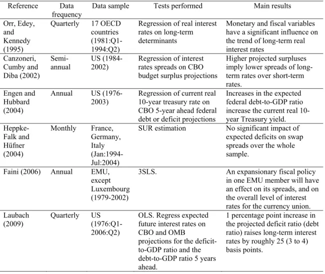
Table 1 offers a summary of some of the findings in the abovementioned related

literature, within different methodological frameworks. Interestingly, from the studies

surveyed, the concern regarding the assessment of possible cross-section dependences

and its technical, empirical, and economic implications for the analysis seems to be

essentially absent.

Table 1 – Some existing empirical evidence regarding fiscal determinants of long-term interest rates

Reference Data frequency

Data sample Tests performed Main results

Orr, Edey, and Kennedy (1995)

Quarterly 17 OECD countries (1981:Q1-1994:Q2)

Regression of real interest rates on long-term determinants

Monetary and fiscal variables have a significant influence on the trend of long-term real interest rates Canzoneri, Cumby and Diba (2002) Semi-annual US (1984-2002)

Regression of interest rates spreads on CBO budget surplus projections

Higher projected surpluses imply lower spreads of long-term rates over short-long-term rates.

Engen and Hubbard (2004)

Annual US (1976-2003)

Regression of current real 10-year treasury rate on CBO 5-year ahead federal debt or deficit projections

Increases in the expected federal debt-to-GDP ratio increase the current real 10-year Treasury yield. Heppke-Falk and Hüfner (2004) Monthly France, Germany, Italy (Jan:1994-Jul:2004)

SUR estimation No significant impact of expected deficits on swap spreads over the whole sample.

Faini (2006) Annual EMU, except Luxembourg (1979-2002)

3SLS. An expansionary fiscal policy in one EMU member will have an effect on its spreads, and on the overall level of interest rates for the currency union. Laubach

(2009)

Quarterly US (1976:Q1-2006:Q2)

OLS. Regress expected future interest rates on CBO and OMB

projections for the deficit-to-GDP ratio and the debt-to-GDP ratio 5 years ahead.

1 percentage point increase in the projected deficit ratio (debt ratio) raises long-term interest rates by roughly 25 (3 to 4) basis points.

3. Methodology

In the subsequent empirical analysis, an initial baseline specification for the real

long-term government bond yield, r, can be written as

1

( )

it it it i i it it

r = i −π =α γ+ X +u . (1)

where i is the long-term nominal government bond yield, π is the inflation rate, and X

includes a set of additional explanatory variables. The index i (i=1,…, N) denotes the

country, the index t (t=1,…, T) indicates the period, αi stands for the individual effects

to be estimated for each country i, and uit the disturbances.

An error-correction form for the real long-term interest rates, which move towards

their long-run level with a speed of adjustment δ, is given by

[

]

) (

) (

0

1 1

1 1

it k

j

it i i it it i j it j k

j

j it j it j it

it i X i X v

i − = ∆ − + ∆ + − − − +

∆

∑

∑

= − − − −

= − −

γ α π λ

θ π

β π

where vit are the disturbances.

Specification (1) illustrates a long-run relationship for the long-term real

government bond yield. Among the several long-run factors influencing the long-term

real interest rate that are included in X, we consider such determinants as: the

government balance-to-GDP ratio, the debt-to-GDP ratio, the current account balance

ratio, inflation surprises, the real effective exchange rate, and a liquidity measure.

As mentioned above, financial markets want to differentiate among sovereign debt

issuers due to the existence of different country-specific credit risk and of a non-zero

probability of sovereign default. Therefore, such variables as the government balance

and the debt-to-GDP ratios could convey relevant information regarding a country

credit risk and help in explaining cross-country financial risk premia. On the other hand,

we do not want to expand too much the possible set of variables since we are aiming at

a parsimonious empirical specification, while for the purposes of the subsequent error

correction analysis it is also preferable not to have too may variables.

In addition, such fiscal indicators also allow financial markets to assess the fiscal

future developments in sovereign borrowers and its perceived credit risk, the country’s

long-run solvency, and repayment likelihood. Therefore, relevant information regarding

a country’s debt burden and whether its public finance behaviour is sustainable, or if the

risk for a build-up of government debt arises.2 In other words, they help in gauging

whether a country can make the interest payments on the outstanding stock of

2

government debt, without being necessarily forced into additional borrowing in the

market and embarking in an unpleasant debt arithmetic trap.

Regarding inflation developments, inflation variability is also relevant in order for

market participants to assess whether an environment of low inflation is in place,

notably via the occurrence of inflation surprises. One can hypothesise that since with

high inflation a government tends to unilaterally and partially inflate away from its

fiscal indebtedness, the need for a higher nominal and real long-term bond yield cannot

be discarded. Moreover, expected inflation is also seen as an indicator of

macroeconomic stability, and higher inflation implies higher sovereign risk. Deviations

from past inflation can be assumed from the actual inflation rate, or taken as an average

of past observations.

In addition, the external imbalance of a country, for instance as proxied by the

current account balance-to-GDP ratio, can convey the existence of a gap between saving

and investment and provide expectations regarding a future depreciation of the domestic

currency. Under those circumstances the risk premia demanded by the markets on

sovereign debt may also increase. Moreover, external imbalances tend to be linked to

fiscal imbalances from a long-term perspective, notably when private saving does not

increase sufficiently to offset the effects of increased budget deficits, and then they may

also impinge via such channel on long-term bond yields.3 In addition, real effective

exchange rate developments are linked to a country’s foreign competitiveness while

being also linked to current account balance positions.

Sovereign debt yields also tend to be related to the depth or liquidity of the

respective outstanding bond market. Indeed, liquidity risk is usually inversely related to

the size of the respective market. Therefore, it seems also useful to consider a measure

of liquidity as a possible determinant of long-term government bond yields. Our

liquidity measure, liquidity debt share, is given by the share of outstanding government

debt in country i, in year t, in the overall outstanding government debt of the full set of

countries in our sample:

1 /

N

it it it

i

LIQ Debt Debt

=

=

∑

where the index i=1, …, N indicates the country.

3

Naturally, one has to be aware that full liberalisation and integration of capital and

bond markets was not in place for the entire time sample under analysis. Indeed, capital

markets were gradually liberalised in the 1970s and 1980s. For instance, this was a

mandatory requirement for EU countries at the start of stage two of EMU, in 1994.

Another caveat is the fact that some home bias can arise among investors, for instance,

some institutional investors may face constraints leading to portfolio investments in the

home country. In a stepwise approach we then i) assess cross-country dependences; ii)

test for panel unit roots; iii) estimate the panel cointegration relationships and iv) assess

the respective magnitudes of cointegration.

Afterwards, and once we have estimated the long-run relationships between real

long-term interest rates and their potential determinants via the computation of the

common correlated effect CCE and CCE-MG (Mean Group) estimators (Pesaran,

2006), we also a estimate complete panel error-correction (PECM) models given by

equation (2) with the Pooled Mean Group approach of Pesaran, Shin and Smith (1999).

This framework allows us to assess the adjustment mechanism to a deviation from the

long-run equilibrium relationship along with the short-run dynamics. Note that the

CCE-MG estimator yields consistent estimates even in the presence of common factors

and is the most efficient (Kapetanios and Pesaran, 2007) and robust to alternative

hypotheses of non-stationarity of variables (Coakley et al., 2006).

4. Empirical analysis

4.1. Data

In our analysis we consider, for the period 1973-2008, the following set of 17

OECD countries: Austria, Belgium, Denmark, Finland, France, Germany, Ireland, Italy,

Luxembourg, Netherlands, Portugal, Sweden, Spain, UK, Canada, Japan, and U.S.

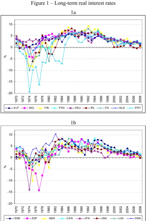
Figure 1 illustrates the development of the long-term real interest rates for those

Figure 1 – Long-term real interest rates 1a -20 -15 -10 -5 0 5 10 19 7 0 19 7 2 19 7 4 19 7 6 19 7 8 19 8 0 19 8 2 19 8 4 19 8 6 19 8 8 19 9 0 19 9 2 19 9 4 19 9 6 19 9 8 20 0 0 20 0 2 20 0 4 20 0 6 20 0 8 %

A UT B EL FIN FRA DEU IRL ITA NLD P RT

1b -20 -15 -10 -5 0 5 10 19 7 0 19 7 2 19 7 4 19 7 6 19 7 8 19 8 0 19 8 2 19 8 4 19 8 6 19 8 8 19 9 0 19 9 2 19 9 4 19 9 6 19 9 8 20 0 0 20 0 2 20 0 4 20 0 6 20 0 8 %

SWE ESP GB R CA N JP N USA LUX DNK

Source: IMF, International Financial Statistics, and authors’ calculations.

From a simple visual inspection we can observe an upward movement in real

long-term interest rates until the beginning of the 1980s, followed by a subsequent

downward trend until the end of the time sample. Real long-term interest rates have

been essentially positive apart from the period of the seventies and early eighties, when

high inflation rates were also prevalent, particularly in such countries as Finland, Italy,

Regarding the liquidity measure that we computed following (3), Table 1 shows

that the U.S. and Japan accounted in 2008 for more than half of the outstanding stock of

sovereign debt in the set of OECD countries considered in our country sample.

We build inflation surprises (πe) taking the difference between actual inflation and

a 2-year moving average of past inflation (see the Appendix for data sources).

Table 1 – Shares of outstanding government debt in the total outstanding debt of the country sample

1970 1980 1990 2000 2008

Austria 0.35 0.90 0.94 0.73 0.88

Belgium 2.02 2.90 2.59 1.44 1.54

Canada 3.84 4.45 3.42 3.27

Denmark 0.85 0.86 0.48 0.39

Finland 0.16 0.19 0.20 0.31 0.31

France 7.41 4.48 4.45 4.38 6.63

Germany 4.74 8.97 7.37 6.53 8.17

Ireland 0.26 0.46 0.45 0.21 0.40

Italy 5.10 8.18 10.90 6.90 8.31

Japan 3.06 18.28 21.19 36.70 28.83

Luxembourg 0.04 0.02 0.01 0.01 0.03

Netherlands 2.88 2.56 2.30 1.19 1.73

Portugal 0.30 0.42 0.33 0.55

Spain 0.73 1.16 2.26 1.98 2.16

Sweden 1.18 1.62 1.02 0.76 0.62

UK 12.13 8.93 3.42 3.49 4.71

US 59.93 36.36 37.16 31.15 31.45

100.00 100.00 100.00 100.00 100.00

Source: European Commission AMECO database and authors’ computations.

4.2. Cross-section dependence

In recent years it has become more widely recognized that the advantages of panel

unit root tests within the macro-panel setting include the use of data for which the spans

of individual time series data are insufficient for the study of many hypotheses of

interest. The adoption of such new panel data methods is preferred to the usual time

series techniques to circumvent the well known problems associated with the low power

of traditional unit root tests. Therefore the body of literature on panel unit root and

panel cointegration testing has grown considerably in the past ten years and now

distinguishes between: first-generation tests (Maddala and Wu, 1999, Levin et al., 2002,

and Im et al., 2003) developed on the assumption of the cross-sectional independence of

panel units (except for common time effects), which is often unrealistic in many

Moon and Perron, 2004, Choi, 2006, and Pesaran, 2007) allowing for a variety of

dependence across the different units. These tests differ according to the way they

eliminate the factorsof structural dependence and the way they aggregate the individual

information.4

Therefore, the first question to deal with is the possible presence of cross-section

dependence in the data. Indeed, as put in evidence for instance, by O’Connell (1998) in

the case of PPP testing, or by Banerjee et al. (2005), panel unit root tests of the first

generation can lead to spurious results (because of size distortions) if there exists

significant degrees of error cross-section dependence and this is ignored. Consequently,

the implementation of second-generation panel unit root tests is desirable only when it

has been established that the panel is effectively subject to a significant degree of error

cross-section dependence. In the cases where cross-section dependence is not

sufficiently high, loss of power might result if second-generation panel unit root tests

that allow for cross-section dependence are used. Therefore, before an appropriate

choice of a panel unit root test is made it is crucial to provide some evidence on the

degree of residual cross-section dependence.

One way of testing for the presence of cross-section dependence in the data is to

carry out the test of Pesaran (2004) and to compute the Cross section Dependence (CD)

statistic. The test of Pesaran (2004) is based on a simple average of all pair-wise

correlation coefficients of the OLS residuals (eit) obtained from standard augmented

Dickey-Fuller (1979) regressions for each individual in the panel. Denoting by ρˆ the _ij

sample estimate of the pair-wise correlation coefficient for the residuals for countries i

and j calculated over T periods, we get:

2 1/ 2 2 1/ 2

1 1 1

ˆ ˆ / ( ) ( )

T T T

ij ji it jt it jt

t t t

e e e e

ρ ρ

= = =

   

= _{=    }



∑

∑

∑

The test statistic proposed by Pesaran (2004), which does not depend on any

particular spatial weight matrix when the cross-sectional dimension (N) is large, is given

by

4

      − =

∑ ∑

CD ρ , (5)

and under its null hypothesis of cross-sectional independence it has asymptotically a

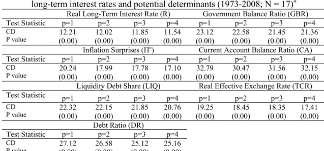
standard normal distribution. The results reported in Table 2 provide evidence in favour

of the existence of cross-sectional dependence in the data since for all series the CD

statistics are always highly significant whatever the number of lags (from 1 to 4)

included in the ADF regressions. In other words, one rejects the null hypothesis of

cross-section independence

Table 2 – Cross-section correlations of the errors in the ADF(p) regressions of real long-term interest rates and potential determinants (1973-2008; N = 17)#

Real Long-Term Interest Rate (R) Government Balance Ratio (GBR)

Test Statistic p=1 p=2 p=3 p=4 p=1 p=2 p=3 p=4

CD P value 12.21 (0.00) 12.02 (0.00) 11.85 (0.00) 11.54 (0.00) 23.12 (0.00) 22.58 (0.00) 21.45 (0.00) 21.36 (0.00) Inflation Surprises (Πe) Current Account Balance Ratio (CA)

Test Statistic p=1 p=2 p=3 p=4 p=1 p=2 p=3 p=4

CD P value 20.24 (0.00) 17.99 (0.00) 17.78 (0.00) 17.10 (0.00) 32.79 (0.00) 30.47 (0.00) 31.56 (0.00) 32.15 (0.00) Liquidity Debt Share (LIQ) Real Effective Exchange Rate (TCR)

Test Statistic _{p=1 p=2 p=3 p=4 p=1 p=2 p=3 p=4}

CD P value 22.32 (0.00) 22.15 (0.00) 21.85 (0.00) 20.76 (0.00) 19.25 (0.00) 18.45 (0.00) 18.35 (0.00) 17.41 (0.00) Debt Ratio (DR)

Test Statistic p=1 p=2 p=3 p=4

CD P value 27.12 (0.00) 26.58 (0.00) 25.12 (0.00) 25.16 (0.00)

Note: Under the null of cross-sectional independence the CD statistic is distributed as a two-tailed standard normal. # Results based on the test of Pesaran (2004).

The variable Inflation Surprises is calculated for each country as the difference between actual inflation and a moving average of two periods.

4.3. Panel unit root testing

Having put in evidence the presence of cross section dependence in real long-term

interest rates, we now turn to the determination of the degree of integration of the series

(real long-term interest rate, government balance ratio, current account balance,

inflation surprises, real effective exchange rate, liquidity debt share, debt ratio) in our

panel of 17 countries, using two second-generation panel unit root tests.

The first 2nd generation unit root test that we use is the test by Pesaran (2007) who

suggests a simple way of getting rid of cross-sectional dependence that does not require

the estimation of factor loading. His method is based on augmenting the usual ADF

cross-sectional dependence that arises through a single-factor model. The resulting

individual ADF test statistics (CADF) or the rejection probabilities can then be used to

develop modified versions of the t-bar test proposed by Im et al. (2003), such as the

Cross-sectionally augmented IPS ( 1 1 N

i i

CIPS N− CADF

=

=

∑

CIPS statistic (CIPS*) where the individual CADF statistics are suitably truncated to

avoid undue influences of extreme outcomes that could arise when T is small (between

10 and 20), or the inverse normal test (or the Z test) suggested by Choi (2001) that

combine the p-values of the individual tests (CZ). Critical values reported in Pesaran

(2007) are provided through Monte Carlo simulations for a specific specification of the

deterministic component and depend both on the cross-sectional and time series

dimensions. The null hypothesis of all tests is the unit root.

The second set of unit root tests of the 2nd generation are the bootstrap tests of

Smith et al. (2004), which use a sieve sampling scheme to account for both the time

series and cross-sectional dependencies of the data through bootstrap blocks. The

specific tests that we consider are denoted t, LM _, max_{, and min .} t _{is the bootstrap}

version of the well known panel unit root test of Im et al. (2003),

1

1 N

i i

LM N LM

−

=

=

∑

mean of the individual Lagrange Multiplier (LMi) test statistics, originally introduced

by Solo (1984), max is the test of Leybourne (1995), and min = 1

1 N

i i

N min

−

=

∑

powerful) variant of the individual Lagrange Multiplier (LMi), with

min_i =min(LM_fi,LM_ri), where LM and LM_{fi ri} are based on forward and backward

regressions (see Smith et al., 2004 for further details). We use bootstrap blocks of

m=20.5All four tests are constructed with a unit root under the null hypothesis and

heterogeneous autoregressive roots under the alternative, which indicates that a

rejection should be taken as evidence in favour of stationarity for at least one country.

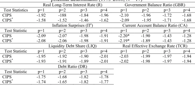
The results of the second generation panel unit root tests proposed by Pesaran

(2007) are reported in Table 3 and provide support of the existence of a unit root in all

series under consideration. This conclusion, which is robust to the number of lags

introduced in the ADF regressions (from p=1 to 4), should be considered as safe given

5

the large and significant degree of cross-section dependence in all series documented in

Table 2.

Table 3 – Panel unit root tests of Pesaran (2007) for real long-term interest rates and potential determinants (1973-2008; N = 17)

Real Long-Term Interest Rate (R) Government Balance Ratio (GBR)

Test Statistics p=1 p=2 p=3 p=4 p=1 p=2 p=3 p=4 CIPS CIPS* -1.92 -1.58 -188 -1.52 -1.84 -1.46 -1.96 -1.62 -2.10 -2.09 -1.96 -1.95 -1.72 -1.71 -1.68 -1.68 Inflation Surprises (Πe) Current Account Balance Ratio (CA)

Test Statistic p=1 p=2 p=3 p=4 p=1 p=2 p=3 p=4 CIPS CIPS* -2.09 -2.08 -2.07 -2.06 -1.98 -1.98 -1.91 -1.91 -2.20* -2.19* -1.90 -1.89 -1.43 -1.43 -1.28 -1.28 Liquidity Debt Share (LIQ) Real Effective Exchange Rate (TCR)

Test Statistic p=1 p=2 p=3 p=4 p=1 p=2 p=3 p=4 CIPS CIPS* -1.95 -1.93 -1.92 -1.91 -1.90 -1.89 -2.01 -2.01 -2.03 -2.02 -1.99 -1.98 -1.97 -1.97 -1.94 -1.94 Debt Ratio (DR)

Test Statistic p=1 p=2 p=3 p=4 CIPS CIPS* -1.75 -1.74 -1.68 -1.65 -1.82 -1.82 -1.78 -1.77

Notes: 1) A constant is included in the estimations.

2) Rejection of the null hypothesis indicates stationarity at least in one country. 3) Critical values are respectively of -2.40 at 1%, -2.22 at 5%, and -2.14 at 10%. * denotes rejection of the null at the 10 % significance level.

CIPS – Cross-section augmented Im-Pesaran-Shin test. CIPS* – truncated CIPS test.

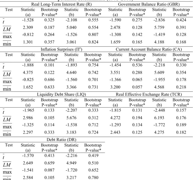
Similar results in Table 4, suggest that for all the series the unit root null cannot be

rejected at any conventional significance level by the four bootstrap tests of Smith et al

(2004).6 Therefore, we conclude that real long-term interest rates and their potential

determinants (government balance ratio, current account balance ratio, inflation

surprisess, real effective exchange rate, liquidity debt share, and government debt ratio)

are non-stationary and integrated of order one at the five percent level of significance in

our country panel. 7

6

The order of the sieve is allowed to increase with the number of time series observations at the rate T1/3 while the lag length of the individual unit root test regressions are determined using the Campbell and Perron (1991) procedure. Each test regression is fitted with a constant term only.

7

Table 4 – Panel unit root tests of Smith et al. (2004) for real long-term interest rates and potential determinants (1973-2008)*

Real Long-Term Interest Rate (R) Government Balance Ratio (GBR) Test Statistic (a) Bootstrap P-value* Statistic (b) Bootstrap P-value* Statistic (a) Bootstrap P-value* Statistic (b) Bootstrap P-value*

t -1.528 0.325 -2.108 0.555 -1.590 0.275 -2.836 0.424

LM 2.309 0.187 5.040 0.554 2.478 0.128 5.759 0.391 max -0.812 0.264 -1.526 0.807 -1.308 0.142 -1.419 0.128

min 1.301 0.357 3.061 0.824 1.659 0.165 4.188 0.168 Inflation Surprises (Πe) Current Account Balance Ratio (CA) Test Statistic (a) Bootstrap P-value* Statistic (b) Bootstrap P-value* Statistic (a) Bootstrap P-value* Statistic (b) Bootstrap P-value*

t -1.888 0.101 -1.893 0.754 -1.454 0.536 -2.218 0.330

LM 4.375 0.122 4.640 0.742 3.551 0.288 5.609 0.354 max -0.825 0.686 -1.560 0.701 -1.366 0.065 -1.955 0.178

min 1.652 0.633 3.366 0.731 3.200 0.057 4.568 0.218 Liquidity Debt Share (LIQ) Real Effective Exchange Rate (TCR) Test Statistic

(a) Bootstrap P-value* Statistic (b) Bootstrap P-value* Statistic (a) Bootstrap P-value* Statistic (b) Bootstrap P-value* t -1.965 0.133 -2.207 0.333 -1.815 0.131 -2.448 0.157

LM 2.986 0.105 5.676 0.312 4.272 0.194 6.193 0.176 max -1.325 0.114 -1.538 0.712 -1.293 0.134 -1.772 0.189

min 2.297 0.333 3.183 0.724 2.443 0.125 4.275 0.182 Debt Ratio (DR)

Test Statistic (a) Bootstrap P-value* Statistic (b) Bootstrap P-value* t -1.570 0.413 -2.216 0.419

LM 2.649 0.659 4.949 0.510 max -1.541 0.087 -1.720 0.652

min 2.584 0.105 3.217 0.780

Notes: (a) Model includes a constant. (b) Model includes both a constant and a time trend.

* Test based on Smith et al. (2004). Rejection of the null hypothesis indicates stationarity at least in one country. All tests are based on 5,000 bootstrap replications to compute the p-values.

Null hypothesis: unit root (heterogeneous roots under the alternative).

4.3. Panel cointegration

Given that all the series under investigation are integrated of order one, we now

proceed with the two following steps. First, we perform 2nd generation panel data

cointegration tests (that allow for cross-sectional dependence among countries) to test

for the existence of cointegration between real long-term interest rates and its potential

determinants. Second, if a cointegrating relationship exists for all countries, we estimate

for each country the cross-section augmented cointegrating regression

) 6 ( ,..., 1 ; ,..., 1 , )

(i X ₁r ₂X u i N t T

by the CCE estimation procedure proposed by Pesaran (2006) that allows for

cross-section dependencies that potentially arise from multiple unobserved common factors.

The cointegrating regression is augmented with the cross-section averages of the

dependent variable and the observed regressors as proxies for the unobserved factors.

Accordingly, rtand Xtdenote respectively the cross-section averages of ri and Xi in

year t. Note that the coefficients of the cross–sectional means (CSMs) do not need to

have any economic meaning as their inclusion simply aims to improve the estimates of

the coefficients of interest. Therefore, this procedure enables us to estimate the

individual coefficients γi in a panel framework.8

In addition, we also compute the CCE-MG estimators of Pesaran (2006). For

instance, for the γ parameter and its standard error for N cross-sectional units, they are

easily obtained as follows:

N

N

i

CCE i MG

CCE

∑

= − − = 1

ˆ ˆ

γ

γ , and

N SE

CCE i N

i MG CCE

) ˆ ( )

ˆ

( 1

− =

−

∑

=

γ σ

γ ,

where γˆ_i−CCEand )σ(γˆ_i−_CCE denote respectively the estimated individual country

time-series coefficients and their standard deviations.

We now use the bootstrap panel cointegration test proposed by Westerlund and

Edgerton (2007). This test relies on the popular Lagrange multiplier test of McCoskey

and Kao (1998), and makes it possible to accommodate correlation both within and

between the individual cross-sectional units. In addition, this bootstrap test is based on

the sieve-sampling scheme, and has the advantage of significantly reducing the

distortions of the asymptotic test. Another appealing advantage is that the joint null

hypothesis is that all countries in the panel are cointegrated. Therefore, in case of

non-rejection of the null, we can assume that there is cointegration between real long-term

interest rates and the potential determinants contained in X. In what follows we consider

the following sets of variables included in X, which cover the main relevant economic

determinants:

8

i) X1= (Πe, CA, DR),

ii) X2= (Πe, CA, GBR),

iii) X3= (Πe, CA, DR, GBR, TCR),

iv) X4= (Πe, CA, DR, LIQ).

The panel cointegration results from the asymptotic tests shown in Table 5,

including a constant term, indicate the absence of a cointegrating relationship between

real long-term interest rates and the different sets of potential determinants for our

country panel. However, this result is based on conventional asymptotic critical values,

calculated on the assumption of cross-sectional independence of countries, an

assumption that is not true here given the significant cross-sectional correlation among

the series documented previously (in Table 2).

Table 5 – Panel cointegration between real long-term interest rates and different sets of potential determinants (1973-2008; N = 17), model with a constant term

LM-stat Asymptotic p-value

Bootstrap p-value # X1= (Πe, CA, DR) 7.430 0.000 0.840

X2= (Πe, CA, GBR) 7.385 0.000 0.782

X3= (Πe, CA, DR, GBR, TCR) 14.168 0.000 0.783

X4= (Πe, CA, DR, LIQ) 9.125 0.000 0.751

Notes: the bootstrap is based on 2000 replications.

a - The null hypothesis of the tests is cointegration of Real Long-Term Interest Rates and potential determinants series.

# Test based on Westerlund and Edgerton (2007).

Therefore, given the existence of some cross-section dependence among

individuals, we used bootstrap critical values.9 In this case the conclusions of the tests

are now more compelling, and retaining a 10% level of significance, we conclude that

there is a long-run relationship between real long-term interest rates and most of the

different sets of potential determinants for our panel of OECD countries. This implies in

particular that over the longer run real long-term interest rates and their determinants

move together in our OECD sample. In addition, Table 5 implies that strictly relying

upon asymptotic critical values (i.e. neglecting cross-sectional dependence) may lead to

wrong (opposite) conclusions about the macroeconomic and fiscal long-run links

between real long-term interest rates and their potential determinants.

9

4.5. The magnitudes of the cointegration relationship

We then estimate equation (6) for the four different sets of variables included in

X to assess the magnitude of the individual γicoefficient in the cointegrating relationship

with the CCE estimation procedure developed by Pesaran (2006), which addresses

cross-sectional dependency. The estimated equations are

1 2 3

e

it i i it i it i it it

r =α γ+ Π +γ CA +γ DR +u , (6a)

1 2 3

e

it i i it i it i it it

r =α γ+ Π +γ CA +γ GBR +u , (6b)

1 2 3 4 5

e

it i i it i it i it i it i it it

r =α γ+ Π +γ CA +γ DR +γ GBR +γ TCR +u , (6c)

1 2 3 4

e

it i i it i it i it i it it

r =α γ+ Π +γ CA +γ DR +γ LIQ +u , (6d)

with i=1,..., , 1,...,N t= T, and the respective estimation results are reported in Table 6.

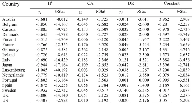
Table 6a – Individual country CCE estimates for 17 OECD countries (1973-2008) between real long-term interest rates and the X1= (Πe, CA, DR) determinants

Country Πe CA DR Constant

γ1 t-Stat γ2 t-Stat γ3 t-Stat α t-Stat Austria -0.681 -8.012 -0.149 -3.725 -0.011 -3.611 3.962 2.907 Belgium -0.850 -14.167 -0.045 -2.682 -0.024 -2.600 -0.281 -2.257 Canada -0.885 -9.725 -0.133 -2.509 -0.032 -2.000 -0.978 -2.736 Denmark -0.645 -4.778 -0.040 -2.727 0.028 2.000 -1.497 -3.749 Finland -0.515 -4.769 -0.006 -0.120 -0.045 -1.957 2.222 3.467 France -0.766 -12.355 -0.176 -3.520 0.049 5.444 -2.234 -3.659 Germany -0.875 -4.581 0.262 2.148 -0.005 -2.167 -4.331 -4.746 Ireland -0.726 -8.643 -0.022 -2.759 0.023 2.300 1.573 2.637 Italy -0.690 -16.429 0.183 2.346 0.121 4.321 -5.388 -3.456 Japan -0.944 -17.164 -0.109 -2.652 -0.047 -2.611 -3.396 -2.741 Luxembourg -1.045 -40.192 0.003 0.029 -0.038 -1.267 -3.200 -2.839 Netherlands -0.779 -10.819 -0.134 -1.523 0.017 3.850 -0.079 -2.034 Portugal -0.803 -13.164 0.114 3.563 0.001 0.000 -0.995 -3.531 Spain -0.875 -13.258 0.058 2.784 -0.007 -1.400 5.189 6.163 Sweden -0.932 -22.732 -0.045 -0.517 -0.140 -5.385 4.017 3.088 UK -0.806 -14.140 0.051 2.125 0.081 3.375 0.267 2.286 US -0.407 -2.928 0.010 2.192 0.020 2.176 3.051 5.202 Note the coefficients of the variables rtandX_1t of equation (6a) have not been reported in the table.

Table 6b – Individual country CCE estimates for 17 OECD countries (1973-2008) between real long-term interest rates and the X2= (Πe, CA, GBR) determinants

Country Πe CA GBR Constant

γ1 t-Stat γ2 t-Stat γ3 t-Stat α t-Stat Austria -0.668 -9.408 -0.147 -3.675 0.027 2.692 2.397 3.405 Belgium -0.796 -12.438 -0.142 -2.407 0.015 2.313 1.109 3.391 Canada -0.821 -8.642 -0.151 -3.283 0.076 2.854 0.680 2.932 Denmark -0.471 -3.680 -0.008 -2.178 -0.357 -1.812 -0.728 -2.874 Finland -0.399 -5.182 -0.039 -2.345 -0.200 -2.597 -0.231 -2.486 France -0.892 -12.389 -0.045 -2.776 -0.100 -2.099 -1.499 -1.669 Germany -0.992 -6.161 0.137 3.593 0.128 2.422 0.461 2.645 Ireland -0.699 -8.034 -0.022 -0.564 0.058 2.289 1.909 3.094 Italy -0.650 -13.000 0.142 2.958 -0.462 -4.200 0.021 2.017 Japan -0.912 -22.244 -0.081 -1.306 0.114 3.081 0.178 3.231 Luxembourg -1.021 -30.029 -0.047 -0.758 0.007 0.092 -2.851 -2.589 Netherlands -0.762 -12.915 -0.028 -0.431 -0.179 -2.210 -0.322 -2.643 Portugal -0.909 -16.527 0.048 1.455 0.199 4.854 0.234 2.600 Spain -0.982 -9.627 -0.146 -2.168 0.175 2.869 0.421 2.636 Sweden -0.990 -14.559 -0.397 -3.970 0.278 3.159 -0.989 -1.169 UK -0.767 -11.984 -0.004 -0.148 0.068 2.194 0.221 2.795 US -0.341 -3.217 -0.132 -2.859 -0.118 -2.532 0.868 2.018 Note the coefficients of the variables rtandX_1t of equation (6b) have not been reported in the table.

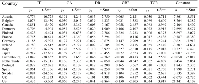
Table 6c – Individual country CCE estimates for 17 OECD countries (1973-2008) between real long-term interest rates and the X3= (Πe, CA, DR, GBR, TCR)

determinants

Country Πe CA DR GBR TCR Constant

γ1 t-Stat γ2 t-Stat γ3 t-Stat γ4 t-Stat γ5 t-Stat α t-Stat

Austria -0.776 -10.778 -0.191 -4.244 -0.015 -2.750 0.065 2.121 -0.030 -2.714 -7.861 -3.551 Belgium -1.076 -13.450 0.050 2.042 -0.039 -4.333 0.021 1.583 -0.069 -4.600 8.764 4.382 Canada -0.851 -5.420 -0.038 -2.369 -0.005 -0.167 -0.058 -2.487 0.063 2.969 -2.404 -4.409 Denmark -0.706 -4.903 -0.087 -2.526 0.020 1.909 -0.166 -2.107 -0.022 -2.917 12.695 5.577 Finland -0.423 -5.494 -0.031 -0.633 -0.039 -2.786 -0.224 -3.733 0.006 0.375 -8.697 -2.077 France -0.745 -10.643 -0.252 -3.360 0.056 3.294 0.011 0.116 -0.047 -2.136 -9.387 -6.380 Germany -1.185 -5.925 0.127 2.221 -0.027 -0.675 0.147 2.909 -0.051 -2.244 -9.621 -7.912 Ireland -0.780 -5.612 -0.057 -2.727 -0.002 -0.105 0.075 2.415 -0.065 -2.140 -3.507 -4.634 Italy -0.733 -16.289 0.178 2.507 0.110 3.929 -0.227 -2.610 -0.115 -2.018 10.527 6.426 Japan -0.917 -17.635 -0.139 -2.106 -0.010 -0.455 0.072 2.323 -0.015 -1.000 -9.007 -5.795 Luxembourg -1.049 -38.852 0.059 1.656 -0.046 -2.769 -0.038 -0.413 0.014 2.560 -10.050 -2.012 Netherlands -0.827 -15.315 0.136 2.333 -0.021 -2.050 -0.044 -0.647 -0.062 -6.889 0.454 2.054 Portugal -0.927 -22.071 0.006 0.109 -0.012 -2.200 0.165 3.667 -0.010 -1.000 1.843 2.376 Spain -0.961 -21.356 -0.114 -2.107 -0.009 -2.250 0.070 2.258 -0.021 -2.750 1.798 2.271 Sweden -0.884 -24.556 -0.158 -2.179 -0.045 -1.818 0.104 2.852 0.026 2.625 3.535 3.399 UK -0.832 -21.333 0.009 0.409 0.101 4.391 0.106 4.417 -0.062 -3.444 -2.073 -2.726 US -0.435 -5.000 -0.066 -2.245 -0.041 -2.864 -0.150 -2.705 0.034 3.919 21.341 4.109

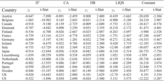
Table 6d – Individual country CCE estimates for 17 OECD countries (1973-2008) between real long-term interest rates and the X4= (Πe, CA, DR, LIQ) determinants

Πe

CA DR LIQS Constant

Country γ1 t-Stat γ2 t-Stat γ3 t-Stat γ4 t-Stat α t-Stat

Austria -0.647 -7.890 -0.091 -2.459 0.008 2.400 -0.439 -3.663 -28.650 -2.304 Belgium -1.063 -18.982 0.145 2.843 -0.031 -2.214 -0.900 -3.180 24.210 2.907 Canada -0.918 -9.180 -0.139 -2.725 -0.009 -2.600 -5.752 -5.321 -10.417 -0.576 Denmark -0.707 -4.842 0.090 2.250 0.053 3.359 -0.218 -2.172 41.473 4.401 Finland -0.536 -6.700 -0.026 -2.667 -0.025 -2.087 -0.263 -3.697 -5.988 -2.528 France -0.759 -13.316 -0.215 -4.778 0.052 3.250 -1.751 -2.447 -47.188 -4.047 Germany -0.899 -5.197 0.191 1.201 0.032 2.744 -0.271 -2.362 -14.353 -5.467 Ireland -0.729 -8.679 0.022 0.786 0.010 2.500 0.420 3.719 -12.185 -3.954 Italy -0.755 -15.729 0.185 2.569 0.222 5.286 -12.00 -3.087 -36.057 -6.857 Japan -0.914 -12.694 -0.056 -2.824 -0.042 -3.680 -0.310 -2.314 -26.735 -7.756 Luxembourg -1.039 -30.559 0.050 0.538 -0.059 -2.458 1.052 3.930 -1.959 -2.053 Netherlands -0.826 -14.000 -0.126 -2.636 0.015 2.556 -0.159 -1.924 -58.738 -4.485 Portugal -0.802 -12.935 0.086 2.867 -0.001 -2.100 -1.460 -2.209 16.218 2.074 Spain -0.950 -20.652 -0.088 -1.846 0.002 2.000 -0.100 -2.632 22.840 3.579 Sweden -0.846 -15.107 0.006 1.067 -0.149 -5.960 0.059 2.458 34.877 3.864 UK -0.820 -14.643 0.052 2.080 0.101 2.629 -12.78 -6.423 8.191 5.334 US -0.522 -3.896 0.030 2.698 -0.024 -3.500 5.151 5.575 -12.222 -3.207

Note the coefficients of the variables rtandX_1t of equation (6d) have not been reported in the table.

From Table 6a we can observe that real long-term interest rates are statistically

and positively affected by changes in the debt-to-GDP ratio for seven out of 17

countries. Regarding inflation surprises they have a negative and statistically significant

effect on real long-term interest rates in all countries. In addition, the effect of the

external imbalances is statistically significant and negative (positive) for nine (five)

countries. In other words, the deterioration of the current account balance would signal

mostly a widening gap between savings and investment and long-term interest rates

may be pushed upwards.

The results of an alternative specification are reported in Table 6b where the

debt-ratio is replaced by the government budget balance debt-ratio. In this case, a better (more

positive) government budget balance reduces the real long-term interest rate in six

countries

In Table 6c, the CCE estimations include simultaneously the two fiscal

determinants of real long-term interest rates, the government budget balance ratio and

the debt-to-GDP ratio, together with current account balances and the real effective

exchange rate. According to the results, improvements in the government budget

balance reduce the real long-term interest rate in seven countries (five in a statistically

effect in ten countries, with a depreciation reducing real long-term interest rates in the

cointegration relationship.

Concerning the relevance of the liquidity of the outstanding government debt,

defined in (3), as a determinant of long-term government bond yields, the related results

are reported in Table 6d, considering the debt-to-GDP ratio as a determinant as well The

effect of an increased country specific sovereign liquidity in the government debt

market contributes to reduce long-term interest rates in 13 cases. In addition, we can

observe that inflation surprises still have a statistically significant negative effect on real

term interest rates in all countries, while higher debt ratios also imply higher

long-term interest rates for nine countries, and current account deteriorations push up real

interest rates in ten cases.

Finally, the results from the common correlated effects mean group (CCE-MG)

method are reported in Table 7. We can see that the estimated long-run relationships for

the real long-term interest rates confirm the statistical relevance of inflation, current

account balances, budgetary balances, government debt and of the liquidity proxy.

Table 7 – Results for common correlated effects mean group (CCE-MG) estimations, 17 OECD countries (1973-2008)

(6a) X1= (Πe,

CA, DR)

(6b) X2= (Πe,

CA, GBR)

(6c) X3= (Πe,

CA, DR, GBR, TCR)

(6d) X4= (Πe, CA,

DR, LIQ)

Constant -0.123 (-4.15)

0.110 (3.96)

-0.091 (-5.26)

-6.216 (-5.28)

Πe

-0.777 (-20.19)

-0.761 (-15.10)

-0.829 (-17.25)

-0.807 (-21.72) CA -0.010

(-3.96)

-0.062 (-5.25)

-0.030 (-4.32)

-0.008 (-4.28) DR -0.060

(-3.27)

-0.137 (-6.25)

-0.009 (-3.36) GBR -0.015

(-3.34)

-0.041 (-2.48)

TCR -0.026 (-3.98)

LIQS -1.749

(-5.35)

Note: t-statistics are in parentheses.

4.6. Estimation of a panel ECM representation

In the previous sub-section we have estimated the long-run relationships

between real long-term interest rates and their potential determinants for our panel of 17

OECD countries, using the common correlated effects mean group (CCE-MG)

and given that there exists a long-run relationship for all countries in our four panel sets,

we turn to the estimation of the complete panel error-correction model (PECM)

described by equation (7):

[

]

1 0

( ) ( ) ( )

p p

it it j it j it j j it j i it it it it

j j

i π β i ₋ π ₋ θ X ₋ λ i ₋ π ₋ α γ X ₋ ε

= =

∆ − =

∑

∑

We use the Pooled Mean Group (PMG) approach of Pesaran, Shin and Smith

(1999), with long-run parameters obtained with CCE techniques, in order to obtain the

estimates of the loading factors λi (weights or error correction parameters, or speed of

adjustment to the equilibrium values), as well as of the short-run parameters βj and θj for

each country of our panel. Consequently, the loading factors and short-run coefficients

are allowed to differ across countries.10

The lag length structure p is chosen using the Schwarz (SC) and Hannan-Quinn

(HQ) selection criteria, and by carrying out a standard likelihood ratio testing-down

type procedure to examine the lag significance from a long-lag structure (started with

p=4) to a more parsimonious one. Afterwards, in order to improve the statistical

specification of the model, we implemented systematically Wald tests of exclusion of

lagged variables from the short-run dynamic (they are not reported here) to eliminate

insignificant short-run estimates at the 5% level. We tested the residuals from each

PECM model for the absence of heteroscedasticity, autocorrelation, ARCH effect, and

we can report that they are not subject to misspecification. The results of the PECM

estimations based on (7) for the different sets of potential determinants previously

considered are reported in Table 8, only for significant short-run estimates at the 5%

level.

10

Note that before considering equation (7), we first used a Wald statistic to test for common parameters across countries (i.e λi= λ, and γi=γ, for i=1,...,N) with the CCE techniques of Pesaran, (2006), that allow

common factors in the cross-equation covariances to be removed. We found that only the null hypothesis

γi=γ, for i=1,…,N was not rejected by data, whereas the speeds of adjustment λi vary considerably across

Table 8a – Panel Error-Correction estimations for rit, X1= (Πe, CA, DR), 1973-2008

∆ rit-1 ∆ rit-2 ∆Πeit ∆Πeit-1 ∆CAit ∆CAit-1 ∆CAit-2 ∆DRit ∆DRit-1 Loading factor λi

Austria -0.20 (-2.21) -0.69 (-7.79) 0.24 (2.91) 0.10 (2.08) -0.06 (-6.31) Belgium -0.69 (-9.34) -0.05 (-2.25) 0.06 (2.05) -0.14 (-3.54) Canada -0.82 (-11.3) -0.03 (-2.78) 0.04 (2.64) -0.10 (-3.36) Denmark -0.62 (-6.31) -0.34 (-1.99) -0.08 (-2.91) Finland -0.51 (-4.35) -0.10 (-3.12) France -0.97 (-4.12) -0.41 (-2.62) 0.73 (3.94) 0.79 (5.11) 0.04 (4.42) -0.35 (-3.48) -0.61 (-4.13) Germany -0.97 (-11.7) 0.43 (3.20) -0.05 (-2.45) -0.38 (-2.79) 0.06 (2.37) 0.39 (3.37) -0.14 (-2.95) Ireland -0.48 (-4.85) -0.09 (-2.79) 0.01 (2.58) 0.08 (2.15) -0.29 (-3.34) Italy -0.84 (-22.4) -0.04 (-3.29) 0.05 (3.31) -0.14 (-3.37) -0.14 (-4.83) Japan -0.76 (-11.2) -0.09 (-3.34) 0.27 (2.78) 0.01 (3.19) -0.29 (-5.36) Luxembourg -1.07 (-11.4) -0.05 (-2.96) 0.06 (2.90) -0.15 (-3.95) Netherlands -0.85 (-16.8) -0.03 (-2.05) -0.39 (-3.22) 0.04 (2.17) -0.09 (-2.38) Portugal -0.69 (-9.02) -0.06 (-2.72) 0.008 (2.56) -0.20 (-3.37) Spain -0.84 (-22.3) -0.03 (-2.56) 0.0045 (2.70) -0.11 (-3.14) Sweden -0.90 (-9.05) -0.06 (-2.16) 0.0074 (2.68) -0.18 (-2.35) UK -0.83 (-13.1) -0.02 (-1.99) -0.06 (-2.84) US -0.50 (-5.39) -0.16 (-3.28) 0.02 (2.74) -0.49 (-4.47) CCE-MG

intercept Πeit-1 CAit-1 DRit-1 -0.123 (-4.15) -0.777 (-20.19) -0.010 (-3.96) -0.060 (-3.27)

Notes: The estimations are obtained from the Pooled Mean Group approach with long-run parameters estimated with CCE techniques. The coefficients of the variables rtandX_1t of equation (6a) have not been reported in the

table. t-statistics are in brackets. r – real long-term interest rate; CA – current account balance; πe – inflation surprises;

Table 8b – Panel Error-Correction estimations for rit, X2= (Πe, CA, GBR), 1973-2008 ∆ rit-1 ∆ rit-2 ∆Πeit ∆Πeit-1 ∆CAit ∆CAit-1 ∆CAit-2 ∆GBRit ∆GBRit-1 Loading

factor λi

Austria -0.53 (-5.81) -0.07 (-2.29) -0.09 (-2.43) -0.21 (-2.53) Belgium -0.68 (-9.31) -0.04 (-2.63) -0.05 (-2.88) -0.12 (-2.99) Canada -0.81 (-10.4) -0.03 (-2.11) -0.04 (-2.17) -0.09 (-2.27) Denmark -0.67 (-7.18) -0.04 (-2.00) -0.50 (-2.74) -0.06 (-2.13) 0.34 (2.84) -0.14 (-2.22) Finland -0.49 (-3.99) -0.07 (-2.86) France -0.76 (-10.7) -0.02 (-2.02) -0.26 (-3.72) -0.03 (-2.13) -0.07 (-2.17) Germany 0.24 (2.03) -0.76 (-12.1) 0.33 (2.57) -0.05 (-2.46) -0.06 (-2.82) -0.15 (-2.94) Ireland -0.04 (-1.99) -0.11 (-2.95) -0.15 (-3.26) -0.35 (-3.65) Italy -0.83 (-22.7) 0.13 (3.04) -0.05 (-3.35) -0.07 (-3.96) 0.20 (2.24) -0.16 (-4.45) Japan -0.47 (-3.6) -0.16 (-2.4) -0.57 (-8.56) -0.23 (-2.07) -0.08 (-3.78) 0.21 (2.25) -0.11 (-4.82) -0.26 (-5.46) Luxembourg -1.04 (-2.02) -0.17 (-3.74) Netherlands -0.83 (-16.6) -0.04 (-2.49) -0.08 (-2.56) -0.39 (-3.38) -0.06 (-2.88) -0.14 (-3.01) Portugal -0.64 (-8.09) -0.07 (-3.16) -0.10 (-3.65) -0.23 (-3.94) Spain -0.81 (-19.7) -0.02 (-2.18) -0.03 (-2.40) -0.09 (-2.46) Sweden -0.77 (-7.69) -0.13 (-2.70) UK -0.83 (-13.2) -0.05 (-2.76) US -0.72 (-8.25) -0.32 (-4.94) 0.39 (2.61) -0.42 (-8.62) CCE-MG

intercept Πeit-1 CAit-1 GBRit-1 0.110 (3.96) -0.760 (-15.1) -0.062 (-5.25) -0.015 (-3.34)

Notes: The estimations are obtained from the Pooled Mean Group approach with long-run parameters estimated with CCE techniques. The coefficients of the variables rtandX_1t of equation (6b) have not been

Table 8c – Panel Error-Correction estimations for rit, X3= (Πe, CA, DR, GBR, TCR), 1973-2008

∆ rit-1 ∆Πeit ∆Πeit-1 ∆CAit ∆CAit-1 ∆DRit ∆DRit-1 ∆GBRit ∆GBRit-1 ∆TCR it ∆TCRit-1 Loading factor λi

Austria 0.14 (2.65) -0.54 (-6.74) 0.24 (2.23) -0.07 (-2.3) -0.09 (-2.36) 0.27 (3.47) 0.11 (2.31) -0.26 (-2.97) Belgium -0.67 (-8.41) -0.03 (-2.16) -0.04 (-2.49) -0.12 (-2.66) Canada -0.86 (-11.9) -0.02 (-2.33) -0.04 (-2.25) -0.10 (-2.96) Denmark -0.70 (-7.78) -0.03 (-2.02) -0.05 (-2.07) 0.33 (2.85) -0.13 (-2.57) Finland -0.50 (-4.11) -0.08 (-2.04) France -0.27 (-3.52) -0.37 (-4.02) -0.97 (-6.25) Germany 0.25 (2.21) -0.84 (-12.6) 0.35 (2.84) -0.03 (-2.17) -0.10 (-2.01) -0.05 (-2.51) -0.13 (-2.93) Ireland -0.56 (-5.58) -0.05 (-2.13) -0.06 (-2.24) -0.18 (-2.68) Italy -0.83 (-25.6) 0.18 (4.66) -0.03 (-2.47) -0.04 (-2.57) 0.17 (2.10) 0.03 (2.71) -0.17 (-3.77) -0.12 (-3.54) Japan -0.31 (-2.78) -0.72 (-11.1) -0.25 (-2.24) -0.07 (-2.84) 0.21 (2.28) -0.12 (-3.21) -0.10 (-3.18) -0.28 (-5.02) Luxembourg -0.94 (-10.0) -0.04 (-2.21) -0.05 (-2.26) -0.15 (-2.92) Netherlands -0.10 (-2.09) -0.82 (-17.3) 0.06 (1.99) -0.16 (-2.07) -0.06 (-2.35) Portugal -0.68 (-8.65) -0.05 (-2.45) -0.07 (-2.94) -0.20 (-3.57) Spain -0.82 (-20.2) -0.03 (-3.02) -0.08 (-3.30) Sweden -0.81 (-9.82) -0.05 (-2.41) -0.16 (-2.81) -0.07 (-2.54) 0.05 (2.22) -0.20 (-3.28) UK -0.91 (-13.4) -0.02 (-2.02) -0.02 (-2.15) -0.07 (-2.52) US -0.36 (-2.80) -0.48 (-5.77) -0.37 (-2.70) -0.10 (-2.59) -0.14 (-2.94) -0.38 (-3.79) CCE-MG

intercept Πe

it-1 CAit-1 DRit-1 GBRit-1 TCRit-1

-0091 (-5.26) -0.892 (-17.2) -0.03 (-4.32) -0.137 (-6.25) -0.041 (-2.48) -0.026 (-3.98)

Notes: The estimations are obtained from the Pooled Mean Group approach with long-run parameters estimated with CCE techniques. The coefficients of the variables rtandX_1t of equation (6c) have not been reported in the