FUNDAÇAo
GETUUO VARGAS
EPGE
Escola de P6s-Graduação
em Economia
Ensaios Econômicos
Escola de
セセMMMMMMMM MMMMMM M
Pós Graduação
em Economia
da Fundação
Getulio Vargas
fi/'
494
ISSN 01 04-891 O
flasticity of substitution between capital and labor: A panel
data approach
Elasticity of Substitution Between Capital and Labor: a Panel
Data Approach
Samuel de Abreu Pessoa' Silvia Matos Pessoa
t
Rafael Rob1
August
18, 2003
Abstract
This paper estimates the price elasticity of the investment-output ratio. The estimating equation follows directly from the long-run solution of the Ramsey-Cass-Koopmans model. It identifies the price elasticity of the investment-output rate with the technical elasticity of substitution between capital and labor. Employing recent dynamic paneI technics we are able to disentangle the short- from the long-run price elasticity as well to identify differences among economies as a fixed effect . Consistent with our aggregative set up, we consider a cross-country paneI for the investment-output rate and the relative price of capital, the explanatory variable. Both are taken from the Penn World Table, comprising 113 economies from 1960 til 1996. Our result points to a 0.7 elasticity of substitution rejecting the Cobb-Douglas specification at 10% confidence leveI. Finally, we show an upward bias on the elasticity estimates whenever cross-country di:fferences are not taken into account.
JEL Classification numbers: D24, D33, E25, 011, 047, 049
Key words: Demand for Investment, Dynamic Panel Data, Elasticity of Substitution.
1 Introduction
This paper estimates the elasticity of substitution between capital and labor and uses it to test the Cobb-Douglas specification. In order to do so, we consider a Ramsey-Cass-Koopmans model with a constant elasticity of substitution (CES) aggregate production function. In steady state, such a model delivers a relation between the investment-output ratio and the relative cost of capital accumulation. The "price" elasticity of this relation is precisely the elasticity of substitution between capital and labor, and that's what we estimate here. The test of the Cobb-Douglas specification is simply a test of the hypothesis that the elasticity is 1. In addition, the intercept1 of the relation between investment-output ratio and relative cost
of capital accumulation captures country specific parameters.
A panel data set was used to estimate the equation characterizing the long-run relationship between the investment-output ratio and the relative cost of the investment good. We take observations of the
*Graduate School of Economics (EPGE), Fundação Getulio Vargas, Praia de Botafogo 190, 1125, Rio de Janeiro, RJ, 22253-900, Brazil. Fax number: (+) 55-21-2553-8821. Email address: [email protected].
tDepartment of Economics, University of Pennsylvania, email address: [email protected].
investment-output rate and of the relative price of capital for 113 economies from 1960 until 1996 from the Penn World Table (PWT) mark 5.8. The panel estimation allows us to estimate cross-country differences in TFP not only as the fixed effect, but also as any non-observed distortion or cost to capital accumulation not taken into account by the PWT data on relative price of capital.
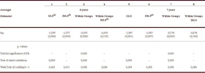
Our annual static estimate of the elasticity of substitution is of 0.5. This result is likely to be biased downward, though, due to the short intervals across observations in our panel. AIso, given that we estimate a long-run relationship employing annual data, the error term is likely to be serial correlated. This problem is addressed in two ways. First, following Chirinko et all (2002) we take long-run averages of the variables. We build two panels that average the data from our original panel over 6 and 7 years. We obtain respectively 0.650 and 0.674 for the within group two stage least square estimation of the elasticity of substitution, and for both panels serial correlation of the error term is rejected. A Wald test rejects the Cobb-Douglas specification at 3% and 10% significance leveIs for the 6- and 7-year average panels, respectively.
Second, following a recent literature on dynamic panel data estimation and considering our original annual panel, we estimate directly the short- and long-run elasticities of substitution. We obtain 0.69 for the long-run elasticity for both the within group and the Aureliano-Bover (1999) estimations. We reject the Cobb-Douglas specification up to 10% of significance leveI for the dynamic panel.
In other words, both solutions to the downward bias problem generate an estimate around 0.7 of the elas-ticity of substitution between capital and labor, and the Cobb-Douglas specification is rejected accordingly.
An important stylized fact emerging from the PWT is that the relative price of capital varies a lot from country to country, and it is negatively correlated with per capita income and the investment rate. Although recent studies in economic growth have acknowledged the importance of differences in Total Factor Produclivily (TFP) lo accounl for income inequalily (Klenow and Rodriguez-Clare (1997), Hal! and Jones (1999), Romer (2001), among olhers) capilal is slil! believed lo play a key role in economic developmenl (Jones (1994) and Resluccia and Urrulia (2001)). This role can be slrenglhened if lechnological change is embodied (Pessoa and Rob (2002)). Given lhal lhe elaslicily of subslilulion is lhe key parameler connecling changes in relative prices into changes in quantities, a study that estimates it directly from cross-country aggregate data seems to be welcome. That is what this paper tries to accomplish.
Restruccia and Urrutia (2001) estimated the very same equation that we do. Differently from our results, theirs strongly support the Cobb-Douglas specification. Although their panel is slightly different from ours (lhey considered 125 counlries from 1960-1985 and lhe dala was laken from lhe PWT mark 5) whal drives the different results is the estimation procedure. They conduced cross-country estimation - for 1960, 65, 70, 75, 80 and 85 - which did not allow them to identify the country specific fixed effect (which requires panel technics). Their results are reproduced by estimating our panel under the assumption that the fixed effect is the same for all countries. As we discuss in Section 5, the non-inclusion of the fixed effect biases upward the elasticity of substitution if highly distorted economies invest less, after controlling for differences in prices of capital. In that situation, the covariation between the omitted variable (country specific effect) and the explanatory variable (relative price of capital) is negative. Collins and Williams (1999) performed a cross-country regression for a set of OECD economies between 1870--1950 and obtained an estimate of 0.7 instead of 1 for the elasticity of substitution. Such result agrees with ours. As we show in Section 5, this agreement is due to the greater homogeneity among the economies considered in their sample, making the cross-country estimation similar to the fixed effect panel estimation.
[1969]). Chirinko et all (2002) is a recent study with a cross-industry static pane! for the USo A!though the results vary a lot, as Chirinko (2002) recent survey shows, it seems that the elasticity of substitution ranges from O to 1. 2,3 Qur estimation of 0.7 is well inside the range yielded by the microdata studies which, given
the aggregate nature of Qur exercise, is the expected resulto
The paper is organized as follows. Section 2 presents the model specification. Section 3 describes the econometric procedure used for estimating the long-run price elasticity of the investment-output ratio and the estimation results are provided in Section 4. Section 5 calculates the bias in the regression of not considering country heterogeneity in the estimation and assesses, based on theory and estimation results, the extent that the price data from the PWT reflects the overall distortion to the capital accumulation decision. Section 6 concludes.
2 Model Specification
The economy is a two-sector economy: sector 1 produces the consumption good and sector 2 the investment good. The capital-labor ratio of both sectors is the same, which means that the relative price of the capital good in units of the consumption good, net of taxes on purchases of capital goods, is constant and given by p, where p-l is sector 2's relative TFP. Additionally, we assume that there is an investment tax whose
proceeds are redistributed back to the household as a lump-sum transference. Letting
T
K = 1+
TK, where TK is the tax rate on investment, it follows that if the household invests It units of consumption good shegets
(T
KP)-1It
units of new capital.The household problem is a standard intertemporal choice. It is given by
subject to
J
=
C'-0max e-pt_t __ dt
1 - I'
o
• -1
Kt
セ@(TKP)
It
-
bKt ,
where the future path of the rental price of capital, rt, the wage rate, Wt, the government lump-sum transfer,
Xt, and the relative price of capital, p, are given.
Under the assumption of an exogenous labor saving technological change, g, we seek a balanced growth path in which the relative price of capital is constant.
The Euler equation that solves the household problem is:
•
Ct 1 [ '
1
-
セ@-
(TKP)
-
r -(p
+
b)
Ct I'
(1)
2 Chirinko (1994) survey covers the early contributions for this literature.
In steady state the resource constraint of the economy is given by:
y
'=AI (k)
セ@A
(h
+
PP- 1Z2)
I (k)
セ@ c+
inv セ@ c+
P
(o
+
g)
k,
where y
==
er;t
is per capita output, c is the flow of consumption, and k is per capita capital, all in efficient units. The term 'inv' is the flow of investment goods in efficient units of the consumption goods (we save letter i for the investment-output rate), lv is the labor share of the v-th sector, and A is the overall TFP, which may vary across countries. Note that we have already substituted into this last equation the equilibrium condition for the investment good: steady state investment,(b
+
g)
k,
is equal to sector 2's output,Ap-1bJ (k).
Let i represent the long-run investment-output ratio as measured by the variable
ki
of the Penn World Table (PWT), investment at constant international prices. As a normalization and without any loss in generality, let us consider that this constant international relative price of investment good is one. We have:. inv 0+ 9 k
1 '=
11
セ@----:4
I
(k)
(2)
The production function
J
is a member of the constant elasticity of substitution (CES) family. For such production function,_ k
セ@
(!'Jfl)-"
I
(k)
Q(3)
where (J is the elasticity of substitution between capital and labor and a: is the capital share. Given that in
steady state the growth rate of consumption is g, from (1) we get the modified golden rule
(4)
Consequently, after substituting
(4)
into (3) and the result into (2), the long-run investment-output ratio is log-linear on price,ゥセ@
o+g [TKPP+O+'(gl-"
A
A
Qso that we can write (for the jth economy)
( 5)
where
lnFEj'=ln[(b+g )( 1 Q
)"l-(l-<r)lnA
j ,TK.i P
+
O+
'(g
(6)
and FE stands for fixed effect.
As pointed out in the Introduction, many scholars have noticed that the relative price of capital is higher in poorer economies. This pattern can be a result of distortions to the acquisition of investment goods either domestically or on overseas purchases due to tariffs and other kinds of trade barriers (Jones (1994)) . Some scholars argue, differently, that this pattern is mainly a result of the relatively lower productivity of poorer economies in the investment good industry as compared to the consumption good industry (Hsieh and Klenow (2003)). 4 In terms of the investment decision, both interpretations lead to the same result: both lead to an increase in the price of capital in units of consumption goods, which is the relevant price for
the investment decision. Consequently, we can assume that pis (to some extent) the result of distortions to capital acquisition and that
T
K is (to some extent) the result of lower productivity in the investmentsector. For estimation purposes the key distinction between p and
T
K is that p denotes any private cost ofinvestment that the PWT price data reflects whereas
T
K does notoIn the folIowing sections we estimate this long-run relation between the investment-output ratio and the relative price of capital.
3 Empírical Implementatíon
Qur main goal is to estimate the short- and long-run price elasticities of investment demand, equation (5). Assuming that alI countries share a common value for the elasticity of substitution, this demand is the same for alI countries apart for an intercept which summarizes the differences in TFP and/or any other policy variable, as expressed by (6). To make this approach operational we have to consider panel data techniques. Models of panel data have gained popularity for several reasons. First, the regression analysis may rely upon higher variability of data as compared to a simple time series or cross-section specifications. Second, we are able to capture the simultaneous variation of time and space dimensions. Third, it alIows the identification of country-specific effects that represent unobserved variables (Aj and TKj ). Furthermore, using panel data we are able to discriminate between the short- and long-run effects of prices on demand for investment. This is done by including the lagged investment as an explanatory variable.
Two econometric models will be used. In the first one we consider a static specification, where the lagged dependent and explanatory variables are not included in the regression equation. In the second one these lagged variables are included. In what folIows both specifications are described.
3.1 Static Panel
We consider the folIowing static representation of the demand for investment:
In ijt = In FEj
+
f3
0 lnpjt + Cjt, Cjt セ@ iid(O, oBセIL@j = 1,2, ... ,N,
t=1,2, ... ,T,
(7)
where In F Ej is an unobserved time-invariant country-specific effect, cu is the error term, and the subscripts j and
t
represent country and time period, respectively. The time period can be a year or an average over either 6 or 7 years.In discussing the techniques to be employed in estimating (7), four issues have to be considered. First, we decided to model the cross-country specific effect as fixed-effects (FE), instead of random-effects (RE), and this decision was based on the results of Hausman test, which rejected the RE specification. Second, in general, errors are heteroskesdastic, which means that they may have different variances across countries. Third, it is likely that our explanatory variable is correlated with Cjt, which means that we have to choose
The FE model is estimated by the Within Groups estimator (WG).5 First we obtain the FE transforma-tion by first averaging equatransforma-tion (7) over time dimension, to get the cross sectransforma-tion equatransforma-tion:
In'j セ@ InFEj +ilolnpj +Ej,
(8)
h I c 1
"T
I . I - 1"T
I d - 1"T
S b ' . (8) f (7)w ere n 'lj = T L...t=l n 'ljt, npj = T L...t=l npjt an Cj = T L...t=l Cjt. u tractmg equatlOn rom
for each
t
gives the FE transformed equation. The WG estimator is then obtained by running OLS on the transformed equation. A RE specification is estimated by GLS random-effects estimator. 6The Hausman test is a test of the equality of the coefficients estimated by the fixed- and random-effects estimators. The latter is only consistent if the country-specific effects are not correlated with the regressors. On the other hand, the FE estimator is consistent regardless of the correlation between the country-specific effects and regressors. If the difference between the two estimates is large then we conclude that there is correlation between the country-specific effects and the regressors. If that is the case, we reject RE hypothesis.
In order to deal with heteroskedasticity we use a robust variance estimator. 7
Our explanatory variable may be correlated with the error termo In particular, we relax the commonly held assumption that the independent variable is strictly exogenous, which means that it is uncorrelated with the error term at alI leads and lags. We consider the lag of regressors as an instrument for it. In order to investigate the correlation between lnpit_l and Cjt we consider the Sargan test of over-identifying
restrictions.
In a static framework, specialIy when working with the annual panel, it is likely that the error terms are serialIy correlated due to the possible omission of relevant variables. In order to investigate this problem, we apply a first-order serialIy correlation testo As we will see, the assumption of no serialIy correlation is rejected for the annual panel. The first attempt to overcome this problem is to consider a variant of the static model in which there is an arbitrary form of serial correlation. In particular, we focus on the first-order serial correlation
(AR(l))
givenby:
0j' セ@ POj'_l
+ Vj"
(9) Vj' セ@ iid(O, HtセIN@The estimation procedure is carried out as folIows. First, the AR(l) coefficient, p, is estimated usmg the
residuaIs from WG estimation. After estimating p, the data is transformed and the AR(l) component is
removed. FinalIy, the WG estimator is applied on the transformed data.
Some researches have proposed another estimation strategy that delivers unbiased estimates without considering regressions based on data at annual frequencies. For instance, Chirinko et all (2002) consider only very low-frequency data variation to estimate the long-run values of their regression variables. By taking
5We could also consider the first-di:lferencing transformation to eliminate the unobserved fixed-e:lfects. However, assuming that êit are serially uncorrelated the WG estimator is more efficient than the first-di:lference estimator.
6See Baltagi (1995), chapter 2.
7This approach was suggested by Arellano (1987). The robust variance estimator of
í3
0 is:N
var(í3o) = (X'X)-l(L: xjÊjÊjXj)(X'X)- l , j=l
where X j = lnPj -lnPj , Êj = (lnij -ln2j) - í3o(lnpj -lnpj) and lnpj is a vector T x l.
interval averages over 6 and 7 years, we are able to estimate the long-run price elasticity of investment using lhe slalie equalion (7) .
As we saw in Section 2, equation (5) establishes a long-run relationship between the relative pnce of capital and the investment-output ratio. Whenever a change in the relative price of investment occurs the economy initiates a dynamic path toward a new steady state. This short-run dynamics is likely to introduce a correlation among contemporaneous investment, its lag, and the lag of price. In order to distinguish between the long-run and the short-run price elasticity of investment, a dynamic panel is required. This will be discussed in the next section.
3.2 Dynamic Panel
As mentioned before, our estimation procedure has to deal with four issues: the presence of unobserved country-specific effects possibly correlated with the regressors, the endogeneity of our explanatory variables, the heteroskedasticity in the error term, and the fact that we work with raw annual data, instead of either smoothing or averaging the series.8 Dynamic panel techniques are therefore required.
Qur panel estimation strategy follows the Generalized Method of Moments (GMM) estimator, proposed by Chamberlain (1984), Hollz-Eakin, Newey and Rosen (1988), Arellano and Bond (1991), Arellano and Bover (1995), and Blundell and Bond (1998a) .
The following is a brief presentation of GMM estimation for dynamic panel data.9 Qur econometric
analysis is based on the following regression equation:10
In ijt セ@ In F E; + {3,ln ijt _ 1 + {32lnPjt
+ (33Inpjt-l
+ fjt,
Ejt セ@ iid(O,0";),
(10)
where In F EJ is the unobserved time-invariant country-specific effect from the dynamic panel, EU is the error
term, and the subscripts j and
t
represent country and time period, respectively. From equation (10) the following short-run and long-run price elasticities of investment demand can be derived118It is important to emphasize that smoothing the data distort the available information whereas averaging the data reduces the amount of information.
9The technical details are discussed further in the Appendix B.
l OIt's important to emphasize that the static AR(I) model is a special case ofthe dynamic model. We can rewrite the AR(I) regression equation as:
Vjt vo iid(O,
a;),
hence, we obtain the same equation if f31 = p, f32 = f3 o, f33 = -f3oP and lnFEf = (1-p)lnFEj.
Short-run price elasticity : {32'
Long-run price elasticity : {3 LR セ@ {32 1 -
+
{3, . {33The usual procedure to eliminate the country-specific effect IS to take first differences of the regresslOn
equation, which for (10) yields
In i jt - In i jt _ 1 セ@ {3, (In i jt _ 1 - In i jt- 2 )
+
{32 (In Pjt - In Pjt-1)+
(33(lnpjt-1 - Inpjt_2)+
fjt - fjt-1·(11)
Assuming that the Ejt are serially uncorrelated (i.e. E(EjtEjs ) = O for
t
#-
s), lnijt_ s are valid instruments in the equations in first differences if s2:
2. This impliesT
-
3 orthogonality restrictions of the form:E(ln ijt_ , (fjt - fjt-1)) セ@ O for s
2'
2;t
セ@ 3, .... , T. (12)Moreover, assuming lnp is weakly exogenous12 we have the following additional moment restrictions: E(lnpjt_ , (fjt - fjt-1)) セ@ O for s
2'
2;t
セ@ 3, .... , T.(13)
Arellano and Bond (1991) develop a consistent GMM estimator based on moment conditions (12) and (13), known as first-differenced GMM estimator. This estimation procedure works well when the instruments are highly correlated with regressors. However, as {31 becomes closer to one or the relative variance of fixed effects (In F EJ) increases, the instruments used in this estimator become less informative, which means that these variables are weak instruments. Instrument's weakness influences the asymptotic and small sample performance of the difference estimator. For instance, Blundell and Bond (1998a) show that the standard first-differenced GMM estimator have large sample bias and poor precision in many simulations experiments.1 3 To reduce the potential biases and imprecisions associated with this estimator they suggest
the use of the Arellano and Bover (1995) estimator in place of the usual one. This alternative estimator combines, in a system, the regression in differences with the regression in leveIs. Their results show that the leveI restrictions remains informative in the cases where the first-differenced instruments become weak. In addition, the recent empirical literature confirms these theoretical and experimental findings.14
In the extended GMM estimator or system GMM, the instruments for the regression in differences are the lagged values of the corresponding leveI variables as before. For the regression in leveIs, the instruments are the lagged differences of the corresponding variables. These are suitable instruments under the following
12The assumption of weak exogeneity of lnpjt means that E(Ej s lnPjt) = O for s> t.
13 Blundell and Bond (1998a) evaluate the performance offirst-dilferenced GMM estimator applying Monte Carlo simulations. In particular, they consider an AR(I) case:
Yit = 7J i
+
O:Yit- l+
Vit·Moreover , they illustrate their results with a dynamic labour demand equation of the form:
additional assumption: there is no correlation between the differences of the right-hand side variables and the country-specific effect, which means that 15
E((lnijt_l-lnijt_2)lnFEf) セ@ O,
E((lnpjt_l -lnpjt_2)lnFEf) セ@ O.
Given lhal E( (In ijt_1 -In ijt_ 2)fjt) セ@ O and E( (lnpjt_l -lnpjt_2)fjt) セ@ O, lhe addilional momenl condilions
are16
E( (In ijt_1 - In ijt_2)(ln FEf + fjt)) セ@ O for
t
セ@ 3, .... , T,eHHャョーェエ⦅ャMャョーェエ⦅RIHャョfeヲKヲェエIIセP@ for エセSL@ .... ,T.
(14)
(15)
An additional advantage of the system GMM over the first-difference GMM estimator is that it allows to study not only the time-series relationship between demand for investment and price but also their cross-section relationship.17
To assess our empirical results we apply two specification tests proposed by Arellano and Bond (1991). The first specification test is the Sargan test of over-identifying restrictions, which tests the overall validity of the instruments. The second test examines the hypothesis that the Ejt are not serially correlated: in the
first-differenced and in the system difference-Ievel regressions we test whether the differenced error term is second-order serially correlated. 18
The last thing we do is to test the validity of additional instruments in the leveI equations. The set of instruments used for the equations in first differences is a subset of that used in the system, so that we can define a specific test of these extra instruments. The "difference" Sargan test addresses this issue by comparing the Sargan statistic for the system GMM estimator and the Sargan statistic for the corresponding first-differenced GMM estimator.
Measurernent Errar. So far, we have not considered the measurement error problem. However, it is a likely problem with our variables and we can easily extend our procedure to accommodate it. Suppose that
In ijt and lnpjt are unobserved variables and we observed only:
15This assumption doesn't imply that there is no correlation between the levels of the lnPjt and lnFEj. In fact, this assumption results from the following stationarity property:
E(lnijt+rnlnFEj) = E(lnijt+nlnFEj) for any m and n,
E(lnPjt+rnlnFEj) = E(lnpjt+nlnFEj) for any m and n.
16 Arellano and Bover (1995) show that further lagged di:lferences would result in redundant moment conditions if all available moment conditions in first di:lferences are exploited.
17The first-di:lferenced GMM estimator eliminates the unobserved fixed e:lfects, which are preserved in the case of the regression in levels.
In
i
jt = In ijt+
mjt,lnpjt = lnpjt
+
ュセエL@(16)
where mjt and ュセエ@ are measurement errors that are uncorrelated with alI In ijt and lnpjt observations and
are uncorrelated across time. Substitution of In ijt and lnpjt from equation (16) in equation (11) yields the
folIowing error term:
セ@tjt - tjt-l セ@ = tjt - tjt-l
+
i i (3(i i )m jt - mjt_l - 1 mjt_l - mjt_2
セ@ HSRHュセエ@ セ@ ュセエ⦅QI@ セ@ HSSHュセエ⦅Q@ セ@ ュセエ⦅RIG@
(17)
By the assumption that the measurement errors are uncorrelated across time,19 we obtain the folIowing moment conditions:
E(ln ijt_ , (fjt セ@ fjt-1)) セ@ O for s
2'
3;t
セ@ 4, .... , T,E(lnpjt_ , (fjt セ@ fjt-1)) セ@ O for s
2'
3;t
セ@ 4, .... , T,E( (In i jt_ 2 セ@ In i jt_3)(ln FEf
+
fjt)) セ@ O fort
セ@ 4, .... , T,E( (Inpjt_2 セ@ Inpjt_3)(ln FEf
+
fjt)) セ@ O fort
セ@ 4, .... , T.(18)
(19)
(20)
(21)
The specification tests for validity of the instruments can also be used to assess whether the control for measurement error is appropriate.
4 Data and Results
To perform our empirical strategy, we make use of the Penn World Table (PWT) data set. We consider a sample of 113 countries20 observed for 37 years, from 1960 to 1996. The relative price of capital in this panel
is the ratio between the price leveI of investment, PWT variable PI, and the price leveI of consumption, PWT variable PC. The investment is the investment share of real GDP per capita at 1996 international prices, PWT variable ki.
We also build two panel derived from our raw panel. In the first we average the data over 6 years: 60-65, 66-71, 71-77, 78-83, 83-89, and 90-95. In lhe second we consider periods of 7 years: 60-66, 67-73, 74-80, 81-88 and 89-96. For the average panel
t
= 1, .. , T, where T = 6 for the 6 years average and T = 5 for the seven years average.We now present the estimation results for the price elasticities of investment demando We organize our discussion according to the empirical specifications introduced above.
19 We could assume that the measurement error follows a moving average process of order 1, in which case we would have to use instruments lagged one more period than what would be necessary if they were serially uncorrelated.
4.1 Static Panel
Annual Panel. The Table 2 considers a static specification, where we exclude the lagged terms as
ex-planatory variables.2 1 In the first two columns, we report the OLS and 2SLS regressions, which ignore the unobserved country-specific effects.
An interesting result that comes out of the first regression is that if we don't controI for FE and for the endogeneity of lnpjtl the estimated price elasticity is -1.000. If we controI for the price endogeneity, this coefficient is -1.026, but the Wald test does not reject -1. Note that all other results deliver an estimated price elasticity well bellow the OLS estimate. In particular, the WG estimation [3] shows that the price elasticity is -0.522. Moreover, correcting for endogeneity we obtain a slightly higher value, -0.558. In addition, the Sargan tests of over-identifying restrictions for 2SLS regressions in columns [2] and [4] do not indicate a problem with the validity of the instrumental variables.
In the last column of Table 2, we estimate equation (7) by GLS random-effects estimator. However, the Hausman test rejects the null hypothesis of no correlation between the RE and the regressors. Consequently, is better to model the country-specific effects as FE.
The first-order serial correlation test is not rejected in the WG regression. In regression [6], we estimate an FE model wilh AR(l) dislurbances. Nole lhal lhe eslimaled coefficienl is lower (-0.385) and lhe eslimaled AR(l) coefficient, p, is 0.725. In addition, the Bhargava et. aI. Durbin Watson test of p = O is rejected. As pointed out before, this particular regression assumes that the short- and long-run price elasticities are the same. Therefore, the estimated coefficients suggest that possibly the short-run and the long-run coefficients are lower and higher than -0.385, respectively, where the estimated f30 corresponds to an approximation of the average value of both elasticities. Moreover, the errors on static regression can be serially correlated if the true relationship is in fact a dynamic one, which would imply that In ijt _ 1 and lnpjt_l were omitted
in the model specification. The brief analysis of this section suggests that it is not reasonable to consider a static panel regression in the context of our raw paneI. We first present the result with the panel that average the data. Then we turn to the dynamic panel estimation.
Average Panel. Table 3 presents the results for the 6 and 7 years average paneI. As expected, they deliver larger values for f3
o,
but still higher than -1. Surprisingly, the WG-2SLS estimation of our annual panel, -0.56 (see column [4] in Table 2) is quite close from the figures for the average panel, either -0.650 for lhe six years average (column [4] in Table 3) or -0.674 for lhe 7 years average (column [8] in Table 3).In order to account for time specific effects, we rerun the previous regressions with time dummies. Table 4 shows lhal if we do nol conlrol for lhe fixed effecl (regressions [1] and [5]) lhe dummies are significanl. Moreover, when we treat price as an endogenous variable, only one time dummy is significant (regressions [2] and [6]). The WG regressions ([3] and [7]) deliver values for
f3
0 very close lo Table 3 and lhe Wald Tesls rejeclf30 = -1. In these regressions none of the serial correlation tests indicate the presence of mis-specification. Moreover, time dummies are significant only when we do not control for price endogeneity. The coefficient estimate for six years average in column [4] suggests a long run price elasticity of -0.66 (robust standard error = 0.16) and the Wald Test rejects -1. Note that all standard errors are higher when we compare Tables 2 (annual panel) with 3 (average panel). In particular, the WG-2SLS robust standard errors are twice the previous values.
21 Ali results in Tables 2, 3, 4 and 5 are computed using Stata 7.0. Only the Test of first order serial correlation is taken from
4.2 Dynamic Panel
Before proceeding to the presentation of the results in Table 6, we first discuss three important issues. First, the existing panel data techniques have been devised and tested considering a microeconomic panel data set, where the time dimension is very 8mall. The asymptotic properties of GMM estimator were derived assuming that N ---t CX) and T is fixed (T
IN
---t O). In this case, the Within Groups and OLS estimators areinconsistent and GMM estimators are consistent . When both tend to infinity, GMM estimator is consistent and asymptotically equivalent to the WG estimator. Alvarez and Arellano (2002) derive the first asymptotic result when
T
IN
tends to a positive constant . They show that WG and GMM exhibit negative asymptotic biases.22 In addition, they report several Monte Carlo simulations where T セ@ N, and the bias of GMMestimator is always smaller than the WG bias. Therefore, for our sample, where T = 37 and N = 113, it seems that GMM estimation is an adequate estimation procedure.
Second, when
T
gets large, the usual GMM procedure that uses alllagged values as instruments becomes unfeasible. Furthermore, some Monte Carlo experiments23 indicate that increasing the number ofinstrumentsused creates a trade-off between the average bias and the efficiency of the estimator. Therefore we decide to concentrate our attention on a "restricted GMM" procedure, in which the number of lagged values used as instruments is small.
Third, ArelIano and Bond (1991) discuss two variants of the GMM procedure:24 the one-step and the
two-step GMM estimators. In the first step, it is assumed that the Ejt are independent and
homoskedas-tic both across units and over time. Consequently, standard errors and test statishomoskedas-tics are not robust to heteroskedasticity. In the second step, these assumptions are relaxed. The residual obtained in the first step is used to construct a consistent estimate of the variance-covariance matrix of the moment conditions. Therefore, if the error terms are spherical, the one-step and the two-step GMM estimators are asymptoticalIy equivalent for the first-differenced estimator. Otherwise, the two-step is more efficient. For system GMM estimator this is always true. However, BlundelI and Bond (1998a) recommend using the one-step results for inference on the coefficients, because the two-step standard errors tend to be biased downward in small samples. Besides, their simulations suggest that the loss in precision that results from not using the more efficient estimator is unlikely to be large. FolIowing the empirical literature, we prefer to report the robust statistics of coefficients and the standard errors for one-step GMM estimator. Moreover, in the context of specification tests, only the Sargan test based on the two-step estimator is heteroskedasticity-consistent and the asymptotic power of the second-order serial correlation test will depend on the efficiency of the GMM estimator. 25 Consequently, we present the specification tests based on the two-step estimator.
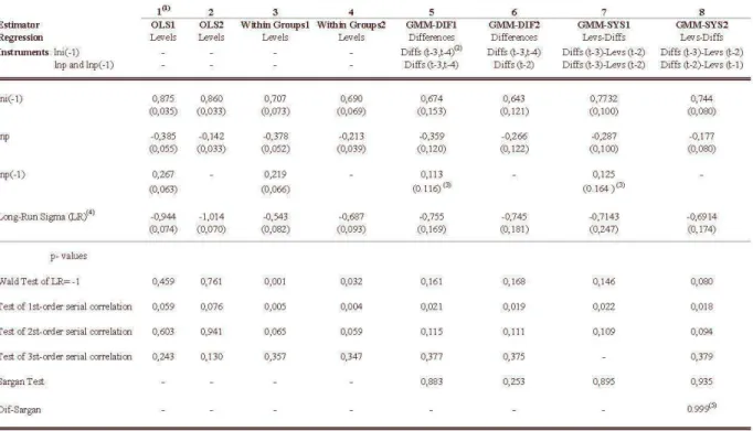
Table 6 reports results of the dynamic panel for several estimators.26 As we will see, the coefficient of
In Pjt-l is not significant in some regressions. Consequently, we decide to present alI results considering two
alternative model specifications: model 1 considers equation (10), where lnpjt_l is included as explanatory variable and in the second model we exclude it. The first four columns of Table 6 report OLS and WG estimates of the parameters {31' {32 and {33 together with estimates of the robust standard error for both
22 However, Alvarez and Arellano (2002) show this result for a first-order autoregressive model with homoskedasticity and only the one-step GMM estimator is considered . The one-step and two-step GMM estimators are discussed in the remainder of the paper and in the Appendix.
23For a Monte Carlo study see Judson and Owen (1996). For a applied cross-country studies see Loyaza, Schmidt-Hebbel and Serven (2000). In addition , Altonji and Segal (1994) and Ziliak (1997) show that this approach reduces the over-fitting biases of the second-step estimates. The two-step estimator is discussed next.
24See the appendix for technical details. 25See Arellano and Bond (1991).
models. As expected, OLS estimates of the lagged dependent variable is biased upwards and the WG estimates is biased downwards. OLS estimator ignores not only the unobserved country-specific effects but also the endogeneity of the explanatory variables. WG estimator deals with the first problem, but still ignores the second one.
Regressions
[51
lo[81
consider lhe GMM eslimalors. In ali GMM regresslOns we decide lo lake lhe conservative approach of allowing for measurement errors that are uncorrelated across time. The validity of lagged leveIst
-
3 andt
-
4 as instruments in the first-differenced equation [5] andt
-
3 as instruments in the first-differenced equations combined with lagged first differenced datedt
-
2 as instruments in the leveIs equations in [7] are not rejected by the Sargan tests. Similarly for regressions [6] and [8] where lnpjt_l is notinduded an explanatory variable.27 As we mentioned before, the presence of second-order autocorrelation
would imply that the GMM estimates are inconsistent. Our tests of second-order serial correlation show that the null hypothesis cannot be rejected.
Note that for the GMM-DIF, the estimated coefficients on the lagged dependent variable are lower than the WG estimates. Following the empiricalliterature, these results suggest that the instruments used in the first-differenced estimator are weak.28
In terms of interpreting the output, the system GMM appears to be more reasonable . The estimated coefficients on the lagged dependent variables are higher than the WG estimates and below the OLS estimates. Moreover, there remains a gain in precision from exploiting the additional moment conditions, and in fact the difference-Sargan statistic that tests the additional moment conditions confirms their validity. Furthermore, our preferred panel estimation procedure, system GMM (GMM-SYS), suggests that lnpjt_l can be omitted
from the specification of the model. In regression [8], the coefficient on the lagged dependent variable is 0.744 and the short-run price elasticity of investment demand is -0.177, which implies a long-run price elasticity of inveslmenl demand (LR) of -0.691 (0.174).29 In addilion, we lesl lhe hypolhesis of LR be equal -1, and this is rejected at 10%.
Finally, note that the WG estimation, regression [4], is very dose to the point estimation delivered by GMM-SYS. Allhough lhe WG eslimalion are biased, as showed by Nickell (1981), Ihis bias is of order セ@
and, consequently, is more detrimental for a micro panel (large
N
and lowT).
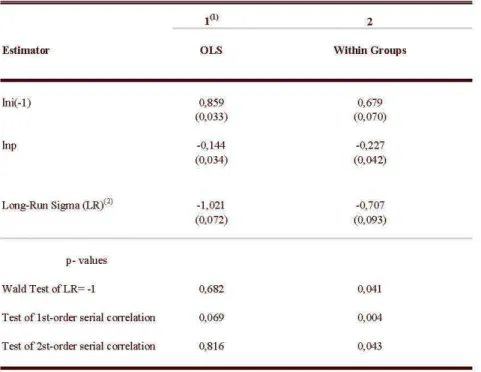
In Table 7 we report OLS and WG estimates of the dynamic equation considering time dummies.30 We
obtain very similar results of those presented in Table 6 (columns [2] and [4] respectively). In particular, the WG estimation delivers a long-run price elasticity of investment demand of -0.707 (0.093).
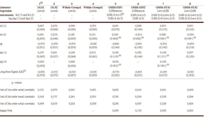
Our last exercise considers a less restricted lag structure of our dynamic equation, which indude a second lag of both explanatory variables. The last two columns of Table 8 report the GMM-SYS estimations of this equation. It turns out that both lagged variables In ijt _ 2 and Inpjt_2 are not significant.
The conclusion that can be derived from these empirical findings is that the lagged investment has a positive and significant coefficient.31 Therefore, the long-run price elasticity of investment demand is more
27In this case, we use the lagged leveI t - 2 as instruments in the first-di:lferenced equation (6) and t - 2 as instruments in the first-dilferenced equations combined with lagged first dilferenced dated t - 1 as instruments in the leveIs equations in (8)
for lnp.
28See Blundell and Bond (1998a).
29The standard error of LR is obtained by using standard approximation techniques. See appendix B.
30 Unfortunately, we could not reproduce the GMM estimates because the total number of instruments would be large relative to the cross-section dimensiono In this case, we do not obtain the two-step GMM estimator, because the matrix W2 =
N
Ci;r
I:
Z1?'ÊjÊj'Z1?)-l, is not invertible. See appendix A.j=l J J
than three times as large as its respective short-run elasticity.32
5 Bias on OLS Estimation
One of the most noteworthy feature of the estimation is that the Cobb-Douglas specification
(O"
= 1) is quite stable across different procedures when one does not control for cross-country differences. In this section we investigate why this is the case and we calculate the bias for not considering the cross-country heterogeneity. In addition, based in the model and in the empirical estimation of the country-specific effect, we assess the extension that the price data of the PWT expresses the costs involved in the investment decision.Lei
i'
==
HゥセL@... ,
ij, ... , ゥセI@ where ij==
(ijl, ... ,Zjt, ... , ijT ) ,and a define p analogously. The variance-covariance matrix of the data is:
[
var(lni) M
セ@
cov (Ini, Inp)Consequently, for the static panel
セols@ cov(lni,lnp)
f3
0 セ@ -1.00 セ@ var lnp ( )cov (Ini, Inp)
var(lnp)
]
[
0.605 -0.307
cov ((In FE
+
f3
0 In p) , In p) var(lnp)-0.307 ] 0.306
cov (In FE, In p)
( )
+f3o·
var lnp
The OLS estimation will bias upward the estimated value of the elasticity of substitution whenever cov(ln FE, In p)
<
O. An analogous (though more involved) logic applies to the dynamic panel. In Appendix C, employing the information of M and assuming that in the first period the economies are at the balanced growth path solution, we show that.---...OL8 {32
+
{32,Bias>
O w h eref3
L R セ@ --'--;'---'--'="'--___1 -
HセL@
+
セBbゥBBI@
.
Actually, if we consider the estimated values for var(lnFED) and for cov(lnFED, lnp), we can calculate
.---...OL8
{3LR directly. We obtain -1.04 which is not far from the estimated value of -1.014 (see table 6, regression
[2]).
Assuming that this logic is correct, if we restrict to a more homogeneous sub-set of economies we should
.---...OL8
get value for (3o that is lower than 1. We take the panel with the average data and select a sub-sample with 15 OECD countries. 33 Table 5 displays the results for the common effect model. As expected, the price elasticity estimates are between -0.52 and _0.76.34
the estimations with and without Sub-Saharan African countries. Overall, the GMM-SYS estimates are pretty stable across experiments and the long-run price elasticity are between the values -0.78 and -0.72.
32Note that the estimated value of /31 (0.744) is quite similar to the estimated p that were obtained in the static AR(I) specifications (0.725).
33Collins and Williams (1999) carried out the same estimation for the 1870-1950 period getting similar results.
Figures 1 and 2 present the scatter plot of
H
セャョゥMャョfe
d@ ⦅ャョゥェエMセLャョゥェエ⦅LMャョfjゥェdェ@
)MMMMMML セLLMMM M M = /--. , In Pj
1-il
11-il
1 t=1, ... ,36 N=1, .. . ,113respectively for the OLS and the GMM-SYS estimations. They illustrate the improvement in the fit when we control for cross-country differences.
6,---,---,
..
4
..
.
.
'
.
.
..
>
LnP
Figure 1: O LS
6
4
2
o
-2
-4
- 1
.
..
R 2= n ?s
V ár (E)=O.39
o LnP 1
Figure 2: SYS-GMM
2
The last exerClse that we perform is to assess the extent that the PWT data on capital reflects the cross-country differences in incentive to capital accumulation. In order to do so, recall equation (6), the expression for the fixed effect delivered by the model
InFEj =ln[(b+ 9) ( 1 Q )"j-(l-O-)lnAj ,
TK,i P
+
b+
1'9 (22)where T K ,i, a non-observable parameter, is the part of the incentive to capital accumulation not accounted
by the price data (recall (4)) . There is evidence that the country-specific TFP, Aj, is high in low price economies. (The relative price of capital is higher in poorer economies (Jones [1994]), and poorer economies presenl lower TFP (Hal! and Jones [1999]).) It follows from (22) lhal, based on lhe sole impacl of Aj on
the fixed effect, we would expect that cov(lnFE,lnp)
2:
O, if (J セ@ 1. But the estimated covariance betweenInFE
andlnp
is negative, indicating that cov(ln TKj , lnp)2:
O and that this covariance is large enough tooutweigh the impact of TFP on the fixed effect. This last result implies that the increase on distortion to capital when one goes from a high income economy to a low income economy is higher than what the PWT data on relative price of capital shows. To assess the cross-country variability of the non-observed parameter
effects.35 The result is that 36
T
K •j E [0.5,41 and that
[
var (In TK )
var (In TK
+
In!»cov (In TK , In]5)
var (In]5) ] [ 0497
124
0.181 ] 0.377 '
where
li
is the vector of cross-time averages. The cross-country variability of PWT data on prices, 0.377, represents roughly 30% of the total cross-country variability of incentives to capital accumulatioll, 1.24.6 Conclusion
The paper presents a series of results indicating that the elasticity of substitution between capital and labor is less than 1. In particular, 0.7 8eems to be the best estimate for such elasticity.
As Chirinko (2002) stressed, this result has important implications for policy, given that the elasticity of substitution is the key parameter connecting changes in incentives to investment decisions. In addition, it should also be relevant for economic quantitative models, especially the RBC literature which has been relying heavily on the Cobb Douglas specification. Last, but not least, there are also non trivial implications for development economics. If the elasticity of substitution is less than one, then the marginal product of capital is bounded at the origin (Barelli and Pessoa [2003]) . Consequently, the demand for capital drops to zero in a very distorted economy, forcing the economy into an absolute poverty trap equilibrium. An economy at the edge of this limit will present a shrinking modern (and relatively capital-intensive) sector coexisting with a traditional sector. Given that the dual economy framework, initiated by Lewis (1954), has recently been rediscovered in a time series setting (Prescott and Hansen [2002]), such poverty trap result is an important consideration to the recent literature .
References
[1] Altonji, Joseph and Lewis Segal 1994. "Small Sample Bias in GMM Estimation of Covariance Structures." NBER Technical Working Paper no. 156.
[2] Alvarez, Javier and Manuel Arellano 2002. "The Time Series and Cross-Section Asymptotics of Dynamic Panel Data Estimators," memo (http://www.cemfi.esrarellano/#WPapers).
[3] Arellano, Manuel 1987. "Computing Robust Standard Error for Within Groups." Oxford Bv1letin of Economics and Statistics, 49: 431-434.
[4] Arellano, Manuel, and Stephen Bond 1991. "Some Tests of Specification for Panel Data: Monte Carlo Evidence and an Application to Employment Equations." Remew of Economic Studies, 58: 277-297.
[51 Arellano, Manuel, and Stephen Bond 1998. "Dynamic Panel Data Estimation using DPD98 for Gauss." Institute for Fiscal Studies, London (http://www.ifs.org. uk/staff/steve _ b.shtml) .
lnFE D
[6] Arellano, Manuel, and Olyrnpia Bover 1995. "Another Look at the Instrumental Variables Esti-mation of Error-Components Models." Journal of Econometrics, 68: 29-51.
[7] Arrow, K. J., H. B. Chenery, B. S. Minhas and R. M. Solow 1961. "Capital-Labor Substitution and Economic Efficiency." Review of Economic and Statistics, 43(3): 225-250.
[8] Baltagi, Badi 1995. &onometric Analysis of Panel Data. New York: John Wiley & Sons.
[9] Barelli, Paulo and Sarnuel Pessoa 2003. "Inada Conditions Imply that Production Function must be Asymptotically Cobb-Douglas." Ensaios Econômicos da EPGE
#
478 (http://www.fgv.br/epge/home/publi/Lista _ anos _ trabalhos.cfm).[10] Blundell, Richard, and Stephen Bond 1998a. "Initial Conditions and Moment Restrictions in Dynamic Panel Data Models." Journalof Econometrics, 87: 115-14
[11] Blundell, Richard, and Stephen Bond 1998b. "GMM Estimation with Persistent Panel Data: an Application to Production Functions." The Institute for Fiscal Policies, Working Paper Series No W99/4 (http://www.ifs.org.uk/workingpapers/wp994.pdf).
[12] Bond, Stephen, Anke HoefRer, and Jonathan Ternple 2001. "GMM
Estimation of Empirical Growth Models." Discussion Paper
#
01/21(http://www.nuff.ox.ac. uk/ economics/ papers/200l/w21/bht 10. pdf).
[13] Charnberlain, Gary 1984. "Panel Data," in: Handbook of Econometrics, Vol 2, Eds: Z. Griliches and M. D. Intriligator, EIsevier, Amsterdam, 1247-1313.
[14] Chirinko, Robert S. 1993. "Business Fixed Investment Spending: Modeling Strategies, Empirical Results, and Policy Implications." Journal of Economic Literature, 31(4): 1875-1911.
[15] Chirinko, Robert S. 2002. "Corporate Taxation, Capital Formation, and the Substitution Elasticity Between Labor and Capital." Emory University, Department of Economics Working Papers
#
02-01 (March) (http://www.emory.edu/COLLEGE/ECON/econgrad/).[16] Chirinko, Robert S., Steve M. Fazzani and Andrew P. Mayer 2002. "That Elu-sive Elasticity: A Long-Panel Approach to Estimating The Price Sensitivity of Business Capital." Emory University, Department of Economics Working Papers
#
02-02 (March) (http://www.emory.edu/COLLEGE/ECON/econgrad/).[17] Collins, Williarns J. and JefITey G. Williarns 1999. "Capital GoodsPrices, Global Capital Markets and Accumulation: 1870-1950." NBER Working Paper No. 7145 (May).
[18] Hall, Robert, and Charles Jones 1999. "Why Do Some Countries Produce So Much More Output per Worker Than Others?" Quarterly Journal of Economics, 114(1): 83-116.
[19] Hansen, Gary and Edward Prescott 2002. "Malthus to Solow." American Economic Review 92(4):
1205-1218.
[21] Hsieh, Chang-Tai and Peter J. Klenow 2003. "Relative Prices and Relative Prosperity." Working Paper (April) (http://www.klenow.com/).
[22] Jones, Charles I. 1994. "Economic Growth and the Relative Price of Capital." Journal of Monetary Economics, 34: 359-382.
[231 Judson, Ruth, and Ann Owen 1996. "Estimating Dynamic Panel Data Models: A PraticaI Guide for Macroeconomists." Federal Reserve Board of Governors.
[24] Klenow, Peter J. and Andrés Rodríguez-Clare 1997. "The Neoclassical Revival in Growth Eco-nomics: Has It Gone Too Far?" NBER Macroeconomics Annual, Ben S. Bernanke and Julio J . Rotem-berg (editors), The MIT Press: 73-103.
[25] Loayza, Norrnan, Klaus Schrnidt-Hebbel, and Luis Serven 2000. "What Drives Private Saving Across the World?" Forthcoming, Review of Economics and Statistics.
[26] Lucas, R. E., Jr. 1969. "Labor-Capital Substitution in US Manufacturing." in The Taxation of Income from Capital, ed. Arnold C. Harberger and Martin J . Bailey, The Brookings Institution, Washington,
D.e.
[27] Lewis, W. A. 1954. "Economic Development with Unlimited Supplies of Labor." Manchester School of Social Science 22: 139-191.
[281 Nickell, Stephen 1981. "Biases in Dynamic Models with Fixed Effects." Econometrica 49(6): 1417-1426.
[29] Pessoa, Sarnuel, and Rafael Rob 2002. "Vintage Capital, Distortions and Development," CARESS Working Paper
#
02-05.[30] Restruccia, Diego and Carlos Urritia 2001. "Relative Prices and Investment Rates." Journal of Monetary Economics 47: 93-121.
[31] Ziliak, Jarnes 1997. "Effcient Estimation with Panel Data When Instruments are Predetermined: An EmpiricaI Comparison of Moment-Condition Estimators." Journal of Bvsiness and Economic Statistics
15(4): 419-431.
A
Dynrunic panel Estimation with GMM
First-differenced GMM. The first two observations of equation (11) are lost to lags and differencing. At
t
= 3, In i j1 is a valid instrument for In i j2 - In i j1 and lnpjl is a valid instrument for Inpj3 - Inpjt2 andInpj2 - Inpjt1. Similarly, at
t
= 4, In i j1 and In i j2 are valid instruments for In ij4 - In ij3 and lnpjl andInpj2 are vaIid instruments for Inpj4 - Inpjt3 and Inpj3 - Inpjt2. Consequently, the instrument matrix has
T - 2
one row for each time period
(T
-
2) andM
= 2 XL
m columns, given by:m=l
('T
o
o
o
o
o
o
1
In
ij1 In ij2 O O O OZD1
セ@J
O O In ij1 In ij2 In ijT - 2
C1"
O O O O O O
1
InPil lnpj2 O O O O
ZD2
セ@J
O O InPil lnpj2 lnpjT_2
Let Xjt = (lnijt,lnpjt,lnpjt_l) be the lxK vector of covariates for i and
t
ande
the K xl vector ofcoefficients. Define the first-differenced versions as:
In
ZJ3 -In
ZJ2(
X
j3 -X
j21
(
Ej3 - Ej2
1
In
ZJ4 -In
ZJ3, x;=
X
j4 -X
j3, and
E;
=Ej4 - Ej3
,;
セ@
( . 1
In ZJT - 'ln ZJT-l XjT - XjT - 1 EjT - tjT-l
The moment conditions (12) and (13) can be written as
E(Z§"fj)
セ@ O, where O is anM
X 1 null vector.The GeneraliZed Method of Moments (GMM) estimator based on these moment conditions minimizes the quadratic distance E*'ZDWZD1 E* for some metric W, where ZDI is the M X N(T - 2) matrix Hzセ@ 1 コセ@ 1 ..
zlJv)
and
E*'
is the N(T - 2) vector(Ei'
1E
2'
1 ...Ej.,i).
This gives the GMM estimator ofe
as:where y*' is a N(T - 2) vector, X* is a N(T - 2) X K. Arellano and Bond suggest two choices for the weights W giving rise to two GMM estimators: one- and two-step estimators. In the one -step estimation it is assumed that the Ejt be independent and homoskedastic both across units and over time, therefore the
N
optimal choice of W is given by W , セ@
(11
L.:
Z§"H
DZ.f)-l,
where HD is a (T - 2) X (T - 2) covariancej=l
matrix of
E(EjEj') :
2 -1 O O O
-1 2 -1 O O
hdセ@
O O O 2 -1
O O O -1 2
In addition, we obtain the variance-covariance estimator of the parameter
e
that is robust to heteroskedas-ticity:N
where
Êj
is the estimated residuaIs.In the two-step estimator the previous assumptions about Ejt is relaxed. In the first-step we obtain the
Êj
and there are used to construct a consistent estimate of the variance-covariance matrix of the momentN
conditions. In this case, the optimal choice of W is given by W 2 = Hセ@
z=
Zf'ÊjÊj' Zf)
-1. j=lHowever, both GMM estimators are consistent for large N and finite T, and they may differ in their asymptoticallyefficiency. Note that, in the special of i.i.d disturbances both are asymptotically equivalent. Systern GMM. The additional moment conditions (14) and (15) can be expressed as:
L' E(Z Ej) セ@ O,
where:
( "i'
Y;3 O O O ,!',lnpj2 O ,!',lnpj3 O O O1
ZL,
セ@.
O O Y;T-1 O O ,!',lnpjT_l
with
.6.
In Pjt = In Pjt - In Pjt-1. N ow, we can construct a GMM estimator which exploits both set of moment conditions. The instrument matrix for the system GMM can be written as:Zj
セ@
(zt
zOf)
The system GMM estimator combines both sets of moment conditions:
çj
セ@( EE',' )
Note that, there is no one-step GMM estimator that is asymptotically equivalent to the two-step estimator, even though in the case of iid disturbances. The natural candidate for weigthing matrix in the one-step
N
estimator is
wfYS
= Hセz]zェhzェIMャL@ whereH:
j=l
which is always asymptotically inefficient relative to two-step estimators because with leveIs equations in-cluded in the system, the optimal weighting matrix depends on unknown parameters
The construction of the two-step GMM estimator is then analogous to that describe above and we use
セ@ セL@
Hj
セ@çjçj
B
Estimated Standard Error of the Long-Run Price Elasticity
In order to compute the estimated standard error of the long-run price elasticity of investment demand (LR), we apply lhe Delta Melhod. Define
f3
セ@(f3
"
f3
2,f3
3 )', lhus a linear Taylor series approximalion oflrHセBセRGセSI@
around lhe lrue parameler vectorf3
is:where:
1
1-/31
(23)
1_1/31 ] .
The variance of the nonlinear function is approximately equal to the variance of the right-hand side of (23), which is:
where var(,8) is the estimated variance matrix of
f3
:
[
カ。イHセLI@
covHセB@
セRI@
var(í'J)
セ@
covHセQG@
セRI@
カ。セセRQ@
cov(f3
"
f3
3 )cov(f3
2,f3
3 )C
The Bias of the OLS Estimation
Assuming that the price is a true exogenous variable it follows that
where
[
1X'
In i123x((T-1)N)
lnp12
and
FE'
セ@
[iョfeセ@
1x((T-1)N)
セ@
(1 )-' 1
f3
Bias = plim -XiX - X/FE,N--+= N N
1
- D
InFE,
1 In ij2
lnpj2
- D
InFEj
1 In ijT
lnpjT
- D
InFEj
1 In iN2 lnpN2
- D
InFEN
iョfeセ@
l,
N
iョfeセ@
'= InFEi -11
L.:
InFEf is lhe cenlralized fixed effecl for lhe j-lh economy (lhe firsl observalionj'=1
Evaluating X'FE, we have
Assuming
we have
セxGfeセ@
NI N --D
fi
LlnFEj
j=l
N T --D
11
L L
In ij,ln F E j j=l t=2, N T --D
fi
L L lnpj'
InFEj
j=l t=2
1 N --D
plim -
I)npj"
InFEj
for anyt, t'
E {I, .. "
T},
N--+=N j=lTo calculate the second term in X'FE we have to take into account the estimated equation. 37 The partial
equilibrium adjustment equation is
In i
j,
セ@ InFEf
+
!l, In ij'_1 - O" (1 - !l,)lnpj'
+
fj"where we substitute for
!l2
( J = - - - - ,
1 - !l,
Integrating on In ijt-l we obtain
Assuming that initially the economies where under the balanced growth path we have
Or,
t t-l t-l
, 1 - !l, D ' ( ) ' \ ' k ' \ ' k
lmj' セ@ 1-!l
lnFEj
-
!l,O"lnpjl- O" 1-!l,L..,!l,lnpj,'-k
+
L..,!l,fj,'-k'
1 k=O k=O
Consequently, we obtain:
N T T t N T N
llャョゥェエャョfeセ@
セ@
L
セ@
=
{3,
LlnFEf
iョfeセ@
- CTL{3;
lャョーェQャョfeセ@
j=l t=2 t=2 (31 j=l t=2 j=l
T t-l N
- CT(l- (3,)
llサSセlャョーェLエMォャョfeセ@
t=2 k=O j=l
T t-l N
+
llサSセleェLエMォャョfeセ@
t=2 k=O j=l
Assuming that
and Ihal
il follows Ihal
where
1 N - D
plim-
L
Ejt
InFEj
セ@ 0, alit,
N--+=N j=l
Qセ@
- DQセ@
- D ,plim
N
L..,Inpjt
InFEj
セ@ plimN L..,lnpjt' InFE j
alit,t
E {1, ...,T},
N--+= j=l N--+= j=l
N N
B "
D - DT-1"
- Dplim - L.., In
FEj
InFEj
-
plimCT--L..,Inpj
InFEj ,
N--+=N j=l N--+= N j=l
Finally, we have:
-COV(I:i,lnp) ] var(lni)
Straightforward calculations lead to
Xセセセs@
( . deiX'X )
-1 2 _ CT+
セセセウ@
(1 -
CT) ( )MLLMMMMMGセセ⦅⦅⦅L⦅@ = phm 3 var In p ,
8cov(FE,p) nセ]nS@
(T-1)
1- HサSセ@+
セHS@ . )1 1,BJas
where we employed the fact that, according to the data,
var (Ini) セ@ 2var (Inp) and var (Inp) セ@ -cov (Ini, Inp).
]f